IDC Technologies Pty Ltd
PO Box 1093, West Perth, Western Australia 6872
Offices in Australia, New Zealand, Singapore, United Kingdom, Ireland, Malaysia, Poland, United States of America, Canada, South Africa and India
All rights to this publication, associated software and workshop are reserved. No part of this publication may be reproduced, stored in a retrieval system or transmitted in any form or by any means electronic, mechanical, photocopying, recording or otherwise without the prior written permission of the publisher. All enquiries should be made to the publisher at the address above.
Disclaimer
Whilst all reasonable care has been taken to ensure that the descriptions, opinions, programs, listings, software and diagrams are accurate and workable, IDC Technologies do not accept any legal responsibility or liability to any person, organization or other entity for any direct loss, consequential loss or damage, however caused, that may be suffered as a result of the use of this publication or the associated workshop and software.
In case of any uncertainty, we recommend that you contact IDC Technologies for clarification or assistance.
Trademarks
All logos and trademarks belong to, and are copyrighted to, their companies respectively.
Acknowledgements
IDC Technologies expresses its sincere thanks to all those engineers and technicians on our training workshops who freely made available their expertise in preparing this manual.
Contents
1
Basic Chemistry
1
1.1
Introduction
1
1.2
Atomic structure
3
1.3
Periodic table
6
1.4
Properties ofelements
8
1.5
Formation of ions
10
1.6
Bonding
13
1.8
Chemical equations
19
1.7
Naming compounds
20
1.9
Atomic weight
22
1.10
Molar Concentration
23
1.11
Oxidation reduction
25
2
Electrochemical Cells
27
2.1
Introduction
27
2.2
Potential difference
28
2.3
Simple voltaic cell
30
2.4
Electrolytic bridge
32
2.5
Electrochemical series
33
3
pH Measurement
37
3.1
Introduction
37
3.2
Properties of water
38
3.3
Definition of pH
38
3.4
Measurement of pH
40
3.5
The measuring electrode
41
3.6
The reference electrode
43
3.7
Nerst equation
48
3.8
Antimony electrode
51
3.9
Sources of error
52
3.10
Applications
57
3.11
Troubleshooting
61
Objectives
When you have completed this chapter you should be able to:
Define the differences between elements, compounds and mixtures
Explain the difference between organic and inorganic chemistry
Describe the structure of an atom
Show how the periodic table is formed and describe the different properties of elements
Show how ions are formed and understand both covalent and ionic bonding
Understand chemical formulae and the use of chemical equations
Explain atomic weight and molar concentrations
Discuss the difference between acids and bases and explain oxidation-reduction
1.1 Introduction
1.1.1 Elements, compounds and mixtures
All substances may be divided into three classifications: elements, compounds and mixtures.
The simplest forms of matter are elements — substances that cannot be split into simpler substances by a chemical reaction. As shown in Figure 1.1, there are over 100 known elements classified in the periodic table and these form the building blocks of all chemicals.
Figure 1.1 The periodic table
A compound is formed by two or more elements which are always combined in the same fixed ratio. Thus, for example, water is a compound of hydrogen and oxygen, shown by its chemical formula H2O, which is always formed from two parts hydrogen and one part oxygen (Figure 1.2). Compounds are often difficult to split into their elements and can only be separated by chemical reactions.
Figure 1.2 Water (H2O) — a compound formed from two parts hydrogen and one part oxygen.
The smallest particle of an element or compound that normally exists by itself and still retains its properties is called a molecule. Normally a molecule consists of two or more atoms — sometimes even thousands. However, as we shall see later, a molecule can also exist as a single atom called a monatomic molecule.
Elements and compounds are pure substances whose composition is always the same. In reality, pure substances are rarely encountered and most are mixtures of compounds or elements that are not chemically combined and in which the proportions of each element or compound are not fixed (Figure 1.3).
Since the elements or compounds making up the mixture each keep their own properties they can usually be separated fairly easily by physical means.
When a mixture has the same properties and composition throughout, (e.g. a mixture of sugar and water in which the sugar is thoroughly dissolved in the water) it is called a homogeneous mixture or a solution.
When the composition and properties of a mixture vary from one part to the other it is called heterogeneous. This might take the form of a suspension in which fine particles of a solid are suspended in a liquid and are not dissolved. Another type of heterogeneous mixture is a two-phase mixture: e.g. a mixture of oil and water in which the oil floats on the water as a separate layer.
Figure 1.3 Various types of mixturesFigure 1.3 Various types of mixtures
1.1.2 Organic and inorganic chemistry
In the study of elements and their components, a distinction is made between what is termed organic and inorganic chemistry.
Originally organic chemistry concentrated on the study of substances found in living organisms. Now, however, it extends to cover all (with a few exceptions) of the compounds of carbon. The vast number of organic compounds (well over two million) include plastics, fibres, drugs, cosmetics, insecticides, foods, etc., and are made possible by the ability of the carbon atom to bond to itself and form a virtually unlimited chain or ring.
Inorganic chemistry is the study of that which is left over — those substances that do not form bonds with carbon.
1.2 Atomic structure
At one time the atom was considered to be the ‘fundamental particle’ — the smallest bit of matter that could be conceived. And indeed, since all atoms of any given element behave in the same way chemically, the atom is the smallest entity to be considered from a chemical viewpoint.
In considering the basic construction of an atom it is usual to consider it as being composed of three elementary sub-atomic particles: protons, neutrons and electrons. It is the number of protons, neutrons and electrons that any atom contains that distinguishes one element from another.
The main mass of the atom comprises the nucleus, which consists of protons and neutrons. The proton has a positive charge and a relative mass of 1 whilst the neutron has a similar mass but no charge.
The nucleus is surrounded by a cloud of electrons each having a negative charge and a mass nearly 2000 times smaller than the proton. In its normal state, an atom has the same number of electrons as protons and is, therefore, electrically neutral.
The simplest structure is the hydrogen atom, which comprises a single proton and a single electron (Figure 1.4).
Figure 1.4 Basic structure of a hydrogen atom comprising a single proton and a single electron.
An element is determined by the number of protons in the nucleus — its atomic number. Since the atomic number defines the element, any atom with 6 protons is carbon, irrespective of the number of neutron or electrons (normally 6 of each).
However, because the number of neutrons in the nucleus may not always be the same as the number of protons, an atom is also defined in terms of the total number of protons and neutrons in the nucleus — called its mass number (not to be confused with its atomic mass). Carbon, for example would normally have 6 protons (atomic number = 6) and 6 neutrons giving a mass number of 12. However, carbon can also exist in other forms, called isotopes, in which the nucleus contains 7 or even 8 neutrons — giving a mass number of 13 or 14 respectively.
The three carbon isotopes are distinguished from one another by writing the mass number after the name of symbol of the element. Thus, as shown in Figure 1.5, carbon with 6 neutrons is called Carbon-12; with 7 neutrons is called Carbon-13; and with 8 neutrons is called Carbon-14.
Figure 1.5 The three isotopes of carbon which are distinguished from one another by writing the mass number after the name of symbol of the element.
Electron shells
With the electrons forming a cloud around the nucleus, the position of any electron is defined in terms of the probability of finding it at some distance from the nucleus. Consequently, it is convenient to visualise the electrons moving around the nucleus of an atom in the same way as planets move around the sun.
This solar-system model visualises the electrons arranged in definite shells or energy levels. Each shell has an upper limit to the number of electrons that it can accommodate and each is built up in a regular fashion from the first shell to a total of seven shells. The first shell can accommodate 1 or 2 electrons; the second shell a maximum of 8; the third a maximum of 18; the fourth 32 and so on with successive shells holding still larger numbers.
In the study of chemistry, it is the electrons in the outermost shell — those which are added last to the atom’s structure — that determine the chemical behavior of the atom. This outer shell is called the valance shell and the electrons in it are called valance electrons. For the first two shells (the first 10 elements) matters are simple and each shell is filled before a fresh one is started. However, in later elements the outer shell develops before the previous one is completed.
Figure 1.6 The full periodic table
Chemical symbols
As shown in Figure 1.1, each element has its own unique symbol that, in most cases, is formed from one or two letters of the element’s English name: e.g. H for hydrogen; He for helium; Li for lithium. Note that the first letter is always capitalised and, where there is a second letter, this is always written in lower case. The symbols of some elements are derived from their Latin names (Table 1.1): Na for sodium from its Latin name Natrium; Au for gold from its Latin name Aurum; Pb for lead from its Latin name Plumbum; etc. An exception to this derivation is tungsten whose symbol W is derived from its German name Wolfram.
Table 1.1 Symbols of elements derived from their Latin names.
Element
Atomic Number
Latin Name
Symbol
Sodium
11
Natrium
Na
Potassium
19
Kalium
K
Iron
26
Ferrum
Fe
Copper
29
Cuprum
Cu
Silver
47
Argentum
Ag
Tin
50
Stannum
Sn
Antimony
51
Stibium
Sb
Gold
79
Aurum
Au
Mercury
80
Hydrargyrum
Hg
Mercury
80
Hydrargyrum
Hg
Lead
82
Plumbum
Pb
1.3 Periodic table
The periodic table (Figure 1.1) is an arrangement of the elements, in order of their increasing atomic numbers, in which a wide range of chemical and physical information is arranged in a systematic way.
As shown, there are seven rows, called periods, with the atomic number increasing by one element from left to right.
The vertical columns or groups are numbered using roman numerals and separate the elements into families having the same number of electrons in the outer shell and similar chemical properties.
As shown in Figure 1.7, about 75% of the elements are made up of what are called metals. Except for mercury, metals are solid and are characterised by high conductivity (both electrical and thermal); high malleability (the ability to be formed or hammered into different shapes); and high ductility (the ability to be drawn into a thin wire).
Figure 1.7 About 75% of the elements are made up of metals
Moving to the right, the elements gradually become less metallic and, on the extreme right (Figure 1.8), are termed non-metals. Non-metals can be solid (carbon being the most commonly observed) liquid (bromine) or gas (oxygen, nitrogen) and generally have poor conductivity, malleability and ductility.
Figure 1.8 Non-metal elements
Somewhere in between the metallic and non-metallic elements are the metalloids (Figure 1.9) that behave mainly like non-metals except that their electrical conductivity, although not good, is closer to metals. These elements are thus often termed semiconductors.
Figure 1.9 The metalloid or semiconductors elements
1.4 Properties of elements
Elements to the extreme left of the periodic table (Figure 1.10), in Group I are, with the exception of hydrogen*, called alkali metals — metals that react with water to form alkaline solutions. All have only one valence electron (one electron in their outer shell) which is easily lost in reactions. Indeed, moving down the group from lithium, sodium, potassium, rubidium, caesium, and francium, their reaction with water becomes increasingly more violent and all need to be stored under oil because of this reactivity.
*Hydrogen owes its location in Group I to its electron configuration rather than its chemical properties.
Figure 1.10 Group I — the alkali metals
The metals of Group II (Figure 1.11) have two fairly loosely bound valance electrons and, although they are also strongly reactive, are not as reactive as Group I elements. Group II elements tend to be found as naturally occurring mineral deposits in the ground or in the sea and are, therefore called the alkaline earth metals.
Figure 1.11 Group II — the alkali earth metals
At the far right hand side of the periodic table (Figure 1.12) are the Group VIII (also know as Group O) elements that form the noble or inert gases. The term noble indicates that the element is chemically inert or inactive.
Figure 1.12 Group VIII — the noble or inert gases
Noble gases – helium, neon, argon, krypton, xenon and radon – all have a full outer shell which accounts for their extreme stability and unwillingness to form compounds. Indeed, at normal temperatures, the lighter noble gases form no compounds whatsoever and exist as monatomic (single-atom) molecules.
In contrast, gases such as hydrogen, nitrogen, oxygen, fluorine, and chlorine react with each other to form diatomic (two-atom) molecules (Figure 1.13) e.g. H2, N2, O2, F2, and Cl2. The Non-metallic elements bromine and iodine also exist as diatomic molecules: Br2 and I2.
Figure 1.13 Hydrogen exists as a two-atom or diatomic molecule (H2)
Another important group that needs to be considered is Group VII – the halogens (Figure 1.14). The elements in this group – fluorine, chlorine, bromine, iodine and astatine – are all non-metals and are characterised by having seven valence electrons.
Figure 1.14 Group VII — the halogens
1.5 Formation of ions
Earlier we stated that the nature of the element is determined by its atomic number – the number of protons within the nucleus – and that it can gain or lose electrons. We also saw how the electrons in an atom are arranged in shells.
Because of the increasing distance of successive shells from the nucleus, the outer electrons are further away from the nucleus and are thus held less tightly. The result is that less energy is required to remove an electron from the 2nd shell than from the 1st shell and still less to remove an electron from the 3rd shell than the 2nd shell. Thus, referring to the periodic table, the energy required to remove an electron from the outer shell of an atom decreases from the top to the bottom (Figure 1.15).
Figure 1.15 The energy required to remove an electron from the outer shell of an atom increases from left to right and decreases from the top to the bottom
In addition, elements to the left of the table have loosely held valence electrons that are easily lost. Now, moving from left to right, as electrons are added to the outer shell, an effectively increasing charge binds them more and more tightly to the nucleus.
It can thus be seen that it is very difficult for elements in the upper right-hand corner to lose electrons and indeed elements with nearly completed shells will tend to attract electrons.
Figure 1.16 shows a sodium atom (atomic number 11) in which the first and second shells are complete and there is one valence electron. Assume now that the atom loses the electron in its outmost shell. What will be the result?
Figure 1.16 Basic structure of a sodium atom
Firstly, since the nucleus has been unaffected and it still has 11 protons (as well as 11 neutrons) it will continue to remain sodium.
The main effect will be that the total charge of the atom will no longer be neutral but will be unbalanced by the absence of the negatively charged electron. The result is that the atom will now have a net positive charge. Since, by definition, an atom is neutral, the change in its charge by losing the electron has, in effect created a new particle called an ion. A positively charged ion is called a cation (pronounced CAT-ion).
The loss of the electron (e–) from the sodium atom creates an ion with a net charge of +1 and the particle’s change in status from a sodium atom to a sodium cation (Figure 1.17) could thus be indicated by the symbol Na1+. In practice the 1 is implied and the symbol is thus written Na+.
Figure 1.17 Formation of sodium cation
If a magnesium atom (atomic number 12) with two valence electrons (Figure 1.16) should lose them, then the resulting cation will be unbalanced by the absence of two electrons and thus have a net positive charge of +2. In this case the particle’s change in status from a magnesium atom to a magnesium cation (Figure 1.18) is indicated by the symbol Mg 2+.
Figure 1.18 Basic structure of a magnesium atomFigure 1.19 Formation of magnesium cation
If we examine the structure of a chlorine atom (atomic number = 17), as depicted in Figure 1.20, it can be seen that the outer (third) shell contains only 7 electrons. And if it should capture an electron and make its outer shell complete (Figure 1.21) its overall charge will become negative. A negatively charged ion is called an anion (pronounced AN-ion).
Figure 1.20 Basic structure of a chlorine atomFigure 1.21 Formation of chlorine anion
The gain of the electron (e– ) into the outer shell of the chlorine atom, creates an ion with a net charge of -1 and the particle’s new status as a chlorine anion is indicated by the symbol Cl– — again with the 1 being implied.
1.6 Bonding
Earlier, we described a compound as a combination of two or more elements. The elements that are combined to form compounds are held together by bonding forces called chemical bonds. The two major bonding forces are ionic bonding and covalent bonding.
1.6.1 Ionic bonding
Ionic bonding is based on the fact that opposite charges attract!
We have already seen how Group I and II elements have loosely held valence electrons that are easily lost and how elements with nearly completed shells will tend to attract electrons.
Thus a sodium atom with a single valence electron will give it up easily to, for example, a chlorine atom with 7 valence electrons (Figure 1.22).
Figure 1.22 Sodium atom gives up an electron easily to a chlorine atom with 7 valence electrons
The sodium cation, with a net charge of +1 and a chlorine anion having a net charge of -1 are attracted to each other and thus form an ionic bond. This ionic bond, formed between a sodium cation (Na+) and a chlorine anion (Cl–), results in the compound sodium chloride (Na+Cl–) or common salt (Figure 1.23). In practice the ionic charges are omitted from the formula which then becomes NaCl.
Figure 1.23 The ionic bond formed between a sodium cation (Na+) and a chlorine anion (Cl–) results in the compound sodium chloride (Na+Cl–)
Another example of an ionic compound formed in this manner is that of magnesium and oxygen. Here, a magnesium cation (Mg2+) having a net charge of +2, combines with an oxygen anion (O2-) having a net charge of -2. The ionic bonding results in the compound magnesium oxide (Mg2+O2-) — normally written as MgO.
Ionic compounds thus exist as a collection of electrically charged positive and negative ions – with each positive ion surrounding itself with as many negative ions as it can, and each negative ion surrounding itself with as many positive ions as it can.
The resulting structure consists of a regular pattern of alternate positive and negative ions, in which no individual molecules can be identified. This regular arrangement of positive and negative ions continues indefinitely in three dimensions throughout the whole structure and is stacked together to form a crystal lattice (Figure 1.24).
Such ionic crystals are hard and brittle with high melting points. Because, at room temperature, the ions are bound and are not free to move, ionic compounds do not normally conduct electricity. However, when melted or dissolved in water, the ions are freed and the materials become conductive.
Figure 1.24 Ionic compounds exist as collections of ions stacked together to form a crystal lattice
The ionic compounds formed in this fashion between metals and non-metals are called salts.
1.6.2 Covalent bonding
Covalent bonding is a more complex arrangement than ionic bonding. Here, the valence electrons are actually shared between the atoms so that each acquires a stable outer shell.
When two atoms of hydrogen are brought together their electrons begin to feel the attraction of both nuclei (Figure 1.25). As the distance continues to decease, there is an increasing probability of finding either electron near either nucleus and at some point, each hydrogen atom shares an electron and the two are thus bonded together to form an H2 molecule. A less accurate, but more easily visualised, analogy is that the electrons form a figure-of-eight path (Figure 1.26) around the two nuclei to form the H2 molecule.
Figure 1.25 When two hydrogen atoms are brought together, at some point a bond is formed and each hydrogen atom shares an electron with the other to form an H2 moleculeFigure 1.26 The electrons can be visualised as forming a figure-of-eight path around the two nuclei to form an H2 molecule
In ionic bonding the ions exist separately. In covalent bonding, however the net molecular charge is neutral. In the case of hydrogen, the covalent bond is formed by a single pair of electrons – with the pair usually connected by a single dash (-):
H – H
Another example of a single-pair covalent bond is chlorine (Figure 1.27). When chlorine atoms approach each other (each with an electron valence of seven) covalent bonding occurs when a pair of electrons are shared (one from each atom) so that each atom now has a stable outer shell of 8 electrons. Again the molecule formed by this single-pair bond is represented by: Cl – Cl
Figure 1.27 Covalent bonding of chlorine atoms occurs when a pair of electrons is shared so that each atom now has a stable outer shell of 8 electrons
Yet another single-pair covalent bond can be formed by, for example, hydrogen and chlorine (Figure 1.28). Here, the pair is made up by one electron from each atom to form a stable outer shell for each. The resulting compound, hydrogen chloride (HCl) is depicted by: H – Cl
Figure 1.28 Single-pair covalent bond formed from hydrogen and chlorine
More than one pair of electrons can form a covalent bond. An oxygen molecule, for example, (with six valence electrons) is formed when two pairs of electrons are shared – again resulting in a stable outer shell of eight electrons for each atom. Here, the double pair is represented by a double dash (=):
O = O
In the case of nitrogen, with five valence electrons, a molecule is formed by a triple bond in which three pairs of electrons (three electrons from each atom) give rise to a stable outer shell for each atom. Here, the triple pair is represented by a triple dash (=):
N = N
Chemical formulae
The most commonly used chemical formula is the molecular formula, which gives the actual composition of a molecule. The molecular formula H2O, for example, indicates that a water molecule comprises two H atoms and one O atom. Similarly, the formula for ethene is C2H4 — indicating that an ethene molecule is made up of two carbon atoms and four hydrogen atoms.
At this point a distinction needs to be drawn between the molecular formula, stated above, and what is termed an empirical formula.
Whilst the molecular formula gives the composition of a molecule, the empirical formula expresses the composition of a substance in terms of whole-number ratios.
Figure 1.29 shows the structure of an ethene molecule. The empirical formula would be written CH2 — indicating the ratio of atoms i.e. there are two hydrogen atoms for each carbon atom. The molecular formula, on the other hand (written C2H4), indicates that a molecule of ethene comprises two carbon atoms and four hydrogen atoms.
For even more information the shortenedstructural formula is used. This shows the sequence of groups or atoms in a molecule. And for more information still, the fullstructural or displayed formula shows all the bonds (both single and double) that make up the molecule.
Figure 1.29 Empirical, molecular and displayed, formulae for ethene
It should be noted that in organic chemistry, even more information than that provided by the displayed formula is required. For example, isomers are compounds having the same molecular formula but different arrangements of atoms in their molecules.
Often, such compounds can only be distinguished from each other using stereochemical formulae that show the structure of the molecule in 3-D.
Thus, whilst the molecular formula for butene is C4H8 it has two different stereochemical formulae (Figure 1.30).
Figure 1.30 Stereochemical formulae illustrates the difference in the molecular formula for butene
We have already seen how some elements such as oxygen and nitrogen occur as simple molecules even when not combined with other elements. These give the formula O2 and N2 respectively.
1.7 Chemical equations
A chemical equation gives a ‘before and after’ picture of a chemical reaction.
In its most basic form, it may be written out:
Sodium + Water → Sodium hydroxide + Hydrogen
The two substances that produce the reaction, and are called reactants, are written on the left hand side of the equation and the result or products of the reaction are written on the right hand side. The + sign stands for ‘react with’ and the arrow (→) stands for ‘reacts to yield’. Thus, the above equation indicates that sodium reacts with water to yield sodium hydroxide and hydrogen.
In practice, the names of the materials involved in the reaction are not written out in full but are replaced by their chemical formulae:
Na + H2O → NaOH + H2
Whilst this equation shows the reaction that takes place, it does not convey the complete picture since closer examination shows that it is chemically unbalanced — i.e. the number of atoms on the one side is not the same as the other (Table 1.2).
Table 1.2 Atoms in formula do not balance
Formula
Na
+
H2
O
→
Na
O
H
+
H2
Number of atoms
1
2
1
1
1
1
2
Totals
4
→
5
In order to balance the equation it may be rewritten as shown with the number in front of each equation, called the coefficient, indicating the number of atoms :
2Na + 2H2O → 2NaOH + H2
Now, an audit, as shown in Table 1.3, show that there is a balance.
Table 1.3 Atoms in formula now balance
Formula
2(Na)
+
2(H2 O)
→
2(Na O H)
+
H2 O
Number of atoms
2(1)
2(3)
2(3)
2
2
6
6
2
Totals
8
=
8
The equation may be extended even further by including what are termed state symbols after each formula that indicate the physical state of each molecule. The state symbols (written in brackets) are:
(s)
=
solid
(l)
=
liquid
(aq)
=
aqueous (solution in water)
(g)
=
gas
Thus, the sodium reaction with water would be:
2Na(s) + 2H2O(l) → 2NaOH(aq) + H2 (g)
Finally, when studying electrolytes in solution, the chemical properties are best represented by an ionic equation which is only concerned with the ions of the participant substances in the reaction.
Thus the reaction:
NaOH(aq) + HCl(aq) → NaCl(aq) + H2O(l)
may be rewritten:
Na+OH–(aq) + H+Cl–(aq) → Na+Cl–(aq) + H2O(l)
Here, Na+, OH– , Cl– and H+ are all ions. Since Na+ and Cl– appear on both sides of the equation, they are uninvolved the ionic reaction and are thus omitted. Now the ionic equation is simply:
Many compounds have trivial names —names that give little information about the structure of the compound. These include names such as salt (NaCl), borax (Na2B4O7·10H2O), chalk (CaCO3), or even proprietary names such as Teflon (F(CF2)nF). In addition, there are other chemical compounds whose names are universally associated with a chemical formula (e.g. water (H2O)). However, most of these names are often difficult to interpret. As a result, most compounds are named using a systematic internationally agreed system.
The compounds of metals and non-metals containing, for example, two different elements are named by first taking the name of the metallic element followed by the main part of the name of the non-metal, which is then modified with the suffix -ide. Thus, the compound of sodium and chlorine takes the metallic element first (sodium) followed by the modified form of chlorine (chloride): i.e. sodium chloride (NaCl).
Other such compounds include:
CaS — calcium sulfide;
MgO — magnesium oxide;
SiN — silicon nitride; and
ZnS — zinc sulfide
When more than two atoms are involved use can be made of a prefix:
mono-
1
di-
2
tri-
3
tetra-
4
penta-
5
hexa-
6
hepta-
7
octa-
8
nona-
9
deca-
10
Thus we get:
CO — carbon monoxide;
CO2 — carbon dioxide
NO2 —nitrogen dioxide;
CS2 — carbon disulfide;
SF6 — sulfur hexafluoride;
GeCl4 — germanium tetrachloride; and
N2O4 — dinitrogen tetraoxide.
Another frequently used suffix is -ate which usually indicates the presence of oxygen. Thus: nitrate, NO3-; sulfate, SO42-; and phosphate, PO43- .
The suffix -ite indicates fewer oxygen atoms than in the corresponding -ate ion, with the prefix hypo- used with the suffix -ite indicating still fewer. The prefix per- indicates more oxygen, or less negative charge, than the corresponding -ate ion. Thus:
Chlorate
ClO3–
Chlorite
ClO2–
Hypochlorite
ClO–
Perchlorate
ClO4–
Certain metals can be found in more than one ionic state. Iron, for example, occurs as either Fe2+ or Fe3+. In such cases, the suffix -ous may be used to identify the lower state and -ic the higher state. Thus:
Fe2+ = ferrous ion
Fe3+ = ferric ion
Cu+ = cuprous ion
Cu2+ = cupric ion
This system of denoting the lower and higher valency states of metal cations has, however, given way to the Stock System in which the oxidation number of the metallic element is indicated by Roman numbers in parenthesis placed immediately after the atom concerned.
The FeCl2 is denoted Iron (II) chloride rather than ferrous chloride and FeCl3 is denoted Iron (III) chloride rather than ferric chloride.
1.9 Atomic weight
Although it is customary to use the term ‘atomic weight’, the term ‘atomic mass’ is more appropriate. Whilst weight is the force exerted on the body by the influence of gravity, mass is a measure of the quantity of matter in a body independent of gravity.
Historically, oxygen was taken as a standard of mass measurement and the oxygen atom was assigned a value of 16.0000 atomic mass units (amu). On this basis, helium was found to have an atomic weight of 4.003 amu, fluorine 19.000, and sodium 22.997.
However, since the early 1960s, the isotope carbon-12 has been used as a standard and the amu is now defined as being 1/12th of an atom of carbon-12 in which:
1 amu = 1.6605665 x 10⁻²⁴ g
In reality the atomic weights based on carbon-12 are in close agreement with those based on natural oxygen.
Table 1.4 compares the atomic weights of the three subatomic particles which show that the atomic weight of the electron is nearly 4000 times less than that of the nucleus and can thus be ignored. In addition, the proton and neutron both have masses close to unity. Since the atomic number is defined as the number of protons in the nucleus, we would expect that the atomic weight would be just over twice that of the atomic number.
Table 1.4 Atomic weights of the three subatomic particles
Particle
Atomic weight (amu)
Proton
1.007276
Neutron
1.008665
Electron
0.0005486
Total
2.0164896
This, in fact, is shown in Table 1.5 which lists the atomic weights of various elements together with their atomic numbers.
Table 1.5 The atomic weights of various elements together with their atomic numbers.
Element
Symbol
Atomic weight (amu)
Atomic number
Hydrogen
H
1.008
1
Helium
He
4.003
2
Carbon
C
12.01
6
Oxygen
O
16
8
Sodium
Na
22.99
11
Chlorine
Cl
35.45
17
Nickel
Ni
58.7
28
Germanium
Ge
72.59
32
Platinum
Pt
195.1
78
Gold
Au
197
79
Uranium
U
238
92
How about the mass of a molecule?
In fact it’s really quite simple. The molecular weight or mass is merely the sum of the atomic weights of each element.
Thus, the molecular weight of water (H2O) would be the sum of the atomic weights of the two hydrogen atoms (1 + 1) and one oxygen atom i.e. 1 + 1+ 16 = 18.
Because there are many substances that do not, in fact, comprise molecules (e.g. salts such as sodium chloride) the term formula weight is often used in place of molecular weight and is calculated in exactly the same way. Thus, the formula weight of sodium chloride (NaCl) would be the sum of the atomic weights of sodium (22.99) and chlorine (35.45) i.e. 22.99 + 35.45 = 58.44.
We saw earlier that an ‘atomic mass unit’ (amu) was defined as having a mass of:
1 amu = 1.6605665 x 10⁻²⁴ g
Alternatively we could say that there were:
6.022 x 10²³ amu = 1g
The figure of 6.022 x 10²³ is referred to as Avogadro’s number and is termed a mole and is given the symbol mol. A mole is a measure of the amount of a substance and 1 mol of any substance contains 6.022 x 10²³ molecules or atoms.
The formal SI definition of a mole is:
“… the amount of any substance that contains as many particles as there are atoms in 12 g of carbon-12. When the mole is used the particles (atoms, molecules, ions, electrons, etc.) must be stated.”
Thus:
One mole of carbon-12 atoms thus has a mass of 12 g.
One mole of oxygen atoms has a mass of 16 g.
One mole of oxygen molecules has a mass of 32 g.
1.10 Molar concentrations
Many chemical reactions are carried out in solution and the concentration is usually defined in terms of the number of moles of the substance (the solute) contained in 1 ℓ of solution. This is called its molar concentration or molarity.
For example, if 10 g of NaCl is dissolved in distilled water to give 1 ℓ of the solution, what is the solution molarity?
We have already determined that the formula weight of NaCl = 58.44 and thus, by definition:
58.44 g of NaCl = 1 mol
Then:
10 g of NaCl
= 0.171 mol
This is the thus the amount of NaCl dissolved in 1 ℓ of the solution and the molarity is 0.171 mol/ℓ.
1.10.1 Acids and bases
Whilst in a purely covalent bond the electrons are shared symmetrically, in most cases the shared electrons tend to be closer to one atom’s nucleus that the other. Such bonds have a partial ionic character in which one part of the molecule has a net positive charge and the other a net negative charge. These molecules are said to be polar.
Figure 1.31 shows a molecule of water in which the shared electrons are more likely to be found around the oxygen atom. The result is that there is a net negative charge on the oxygen atom. And since the electrons spend less time orbiting the hydrogen atoms there is a net positive charge on each hydrogen atom.
Figure 1.31 In a water molecule the shared electrons are more likely to be found around the oxygen atom
It should be noted that, as distinct from ionic bonding, the net charges are less than 1+ or 1-, this being indicated by the symbol (δ).
In pure water, a small number of molecules ionise — each forming a hydrogen ion (H+) and a hydroxide ion (OH–). This reaction is called self-ionisation. Since the number of hydrogen and hydroxide ions is equal, the water is neutral. However, this balance can be upset by a number of compounds that dissolve or react with the water and produce either hydrogen ions or hydroxide ions.
Substances that react in this manner and produce hydrogen ions (H+) in the solution are called acids and those that react and produce hydroxide ions are called bases.
Another name used to describe the hydrogen ion (H+) is proton and thus acids may also be described as proton donors and bases as proton acceptors.
In reality, the hydrogen ions do not exist on their own but are attached to the water molecules to become what are called hydroxonium ions (H3O+). This is shown in the reaction of hydrochloric acid (HCl) with water:
HCl + H2O → H3O+ + Cl–
Nevertheless, because only the hydrogen ion takes part in the reaction in a solution, the H+ ions may be considered as the active ingredient and, for all intents and purposes, the hydroxonium ion may be considered to be a hydrogen ion.
A base has been described as a substance that gives hydroxide ions (OH–) when reacting or dissolving in water. Alternatively, it has been described as a proton acceptor. A base is, therefore, the chemical opposite to an acid. As a result, a base may be further described as a substance that will neutralise an acid by accepting its hydrogen ions.
Thus, in the right proportions, the reaction of hydrochloric acid (HCl) with sodium hydroxide (NaOH) gives:
HCl + NaOH → H2O + NaCl
resulting in a solution containing ordinary table salt.
When a base is dissolved in water the resulting solution contains more hydroxide ions than hydrogen ions and is termed an alkaline. The determination of whether a solution is acidic or alkaline, and their relative strengths, is compared on a pH scale.
1.11 Oxidation-reduction
In our discussions on bonding, we saw how both ionic and covalent bonding involved a shift in electron density from one atom to another.
In the case of sodium chloride (NaCl), for example, an electron was transferred completely from Na to Cl to form the Na+ and Cl– ions (Figure 1.32). This shift in electron density, from one atom to another, is termed an oxidation-reduction reaction — usually shortened to Redox reaction.
Oxidation refers to the loss of electrons during a reaction whilst reduction refers to the gain of electrons. Oxidation and reduction always occur together — with one substance accepting the electrons that another loses. Thus in the reaction of sodium chloride, sodium loses an electron and is therefore oxidised whilst the chlorine atom gains an electron and is said to be reduced.
Figure 1.32 Loss of electrons is called oxidation and gain of electrons is termed reduction
Although in the sodium chloride reaction, the sodium supplies the electron, and is thus oxidised, it acts as the reducing agent. Likewise the chlorine, which is reduced, acts as the oxidising agent.
A measure of the power of a substance to gain electrons is called the Redox potential. A reducing agent that readily loses electrons will have a negative potential whilst oxidising agents will have a positive potential.
Objectives
When you have completed this chapter you should be able to:
Describe the basic principle of the electrochemical cell
Show how a potential difference is formed between two dissimilar electrodes immersed in water
Demonstrate how a simple voltaic cell is formed
Explain how a Daniell cell works
Understand the use of an electrolytic bridge
Discuss the importance of the electrochemical series and how it is applied
2.1 Introduction
If a metallic rod such as zinc is placed in water, there is a tendency for a redistribution of electric charges to take place.
Firstly, the water molecules attract positive ions from the metal. Countering this, however, is the fact that as the positive ions leave the metal, the rod has a tendency to become negatively charged. This results in the positive ions being held to the surface of the rod — with the ions thus being said to be adsorbed onto the surface of the metal (Figure 2.1).
Figure 2.1 When a zinc rod is placed in water, positive ions are adsorbed onto its surface and the rod will have a negative charge
Some of the adsorbed ions may break away from the surface of the metal and the rod will actually lose mass (Figure 2.2). However, because each ion that is lost causes the rod to become more negatively charged this reaction, called desorption, can only happen to a few ions before an equilibrium is rapidly reached.
Figure 2.2 Some of the adsorbed ions break away from the surface of the zinc and it loses mass
The amount of negative charge on such a metal rod placed in water is determined largely by the reactivity of the metal. Zinc atoms ionise easily and thus the negative charge will be relatively high — with a potential difference thus existing across the zinc/solution junction. However, copper atoms, for example, ionise only with some difficulty and thus, as shown in Figure 2.3, the amount of negative charge is considerably less. The result is that the potential difference across the copper/solution junction is also considerably less.
Figure 2.3 A copper rod placed in water will have fewer positive ions adsorbed onto its surface and the rod will have a smaller negative charge
2.2 Potential difference
Assume now that a zinc rod and a copper rod, referred to as electrodes, are both placed in water and a high impedance voltmeter is connected across them (Figure 2.4). As a result of their different electrode potentials, the voltmeter would indicate that a potential difference now exists, between the copper and zinc electrodes, of about 1.1 V.
Figure 2.4 A high impedance voltmeter connected across the electrodes shows a potential difference between them of about 1.1 V
If, instead of the high impedance voltmeter, a conducting wire is connected across the electrodes there will be an initial brief flow of electrons from the zinc electrode to the copper electrode (Figure 2.5). Since the zinc electrode loses electrons it will become less negatively charged whilst the copper electrode will gain electrons and will become more negatively charged.
Figure 2.5 If the electrodes are connected using a conducting wire there will be a brief flow of electrons from the zinc electrode to the copper electrode and the zinc electrode will be less negatively charged and the copper electrode will be more negatively charged
The reduced negative charge of the zinc electrode means that the adsorbed positive ions are now less strongly attached to its surface and may become detached — exposing new atoms. Since this encourages more ionisation, the zinc electrode will again tend to become more negative.
At the copper electrode, the inflow of electrons attract adsorbed copper ions even more and further ionisation is thus discouraged, As a result, both electrodes end up at the same potential and no potential difference will now exist across them (Figure 2.6).
Figure 2.6 After as short time both electrodes end up at the same potential and no potential difference will exist across them
2.3 Simple voltaic cell
One means of overcoming this stalemate is to make the solution acidic (e.g. a dilute solution of sulphuric acid) and thus increase the number of free hydrogen ions (H+) in the solution. As before, ions will continue to leave the zinc electrode — with ionisation still taking place and the excess electrons being conducted through to the copper electrode.
Now, at the copper electrode, the inflow of electrons attracts the positive hydrogen ions, which are adsorbed onto the electrode’s surface and then combine with the electrons to form hydrogen gas, which bubbles to the surface (Figure 2.7). In this manner, a current will continue to flow through the conductor until either the zinc electrode has been completely corroded away or until all the hydrogen ions in the solution (called the electrolyte) have been released as gas at the copper electrode.
Figure 2.7 By making the electrolyte acidic, the inflow of electrons on the copper electrode attracts the positive hydrogen ions which are adsorbed onto the electrode’s surface and combine with the electrons to form hydrogen gas
One of the major defects of this simple voltaic cell is that the liberated hydrogen forms a layer on the copper electrode (Figure 2.7). Apart from considerably increasing the internal resistance of the cell, the copper/solution junction now becomes a copper/hydrogen junction that produces an emf that is in opposition to that produced by the current flow. The result is that on connecting the two electrodes via the conductor to produce a current flow, within a very short time, the emf across the electrodes will fall from about 1.1 V to 0.7 V or even less. This effect is termed polarisation.
2.3.1 The Daniell cell
One method of overcoming this problem is by means of the Daniell cell shown in Figure 2.8 — a modified form of the simple voltaic cell. Here the zinc electrode is again placed in a dilute solution of sulphuric acid (or, more traditionally, zinc sulphate). The difference is that in this case the copper electrode is effectively immersed in a saturated solution of copper sulphate which acts as the depolariser.
Figure 2.8 The Daniell cell — a modified form of the simple voltaic cell —overcomes the problem of polarisation
The cell is redrawn in Figure 2.9 to illustrate the action which shows that, in effect, we now have two half-cells — the zinc electrode in the sulphuric acid forming one half-cell and the copper electrode in the copper sulphate forming the other half-cell. Earlier we had seen how the positive hydrogen ions of the sulphuric acid were used to attract the excess electrons in the copper electrode. In this case, the Cu2+ cations of the copper sulphate (Cu2+SO4) are used to attract the excess of electrons in the copper electrode — with the ions thus deposited as metallic copper on the electrode.
Figure 2.9 In effect, the Daniell cell comprises two half-cells — the zinc electrode in the zinc sulphate forming one half-cell and the copper electrode in the copper sulphate forming the other half-cell
2.4 Electrolytic bridge
The two half-cells are connected ‘electrically’ by the porous pot which prevents any rapid mixing of the two electrolytes but at the same time allows ions to diffuse through it.
If the two solutions were not in contact in this way (Figure 2.10) the electrode reactions would rapidly cease. Zinc cations (Zn2+) leaving the zinc electrode would rapidly build up a positive charge in the electrolyte and ultimately prevent electrons leaving the zinc electrode. Similarly, the adsorption of copper ions on the copper electrode would leave the solution with an overall negative charge (SO42-) that would prevent negative electrons entering the copper electrodes.
Figure 2.10 With the two solutions separated by an impervious barrier, zinc cations (Zn2+) leaving the zinc electrode would build up a positive charge in the electrolyte and thus prevent electrons leaving the zinc electrode. Similarly, the copper electrode would leave its electrolyte with an overall negative charge (SO42-) that would prevent negative electrons entering the copper electrodes
The effect of the porous barrier (Figure 2.11) is thus to allow the negative sulphate anions (SO42-) to pass through the barrier and neutralise the positive zinc cations (Zn2+), and vice versa, so that both the solutions would remain neutral.
Figure 2.11 The porous barrier allows the negative sulphate anions (SO42-) to pass through the barrier and neutralise the positive zinc cations (Zn2+), and vice versa, so that both solutions remain neutral
One of the problems of such a simple porous clay barrier is the fact that different rates of diffusions of the cations and anions can occur across the barrier — giving rise to a liquid junction potential.
This effect can be considerably reduced by using an alternative method of connecting the two half-cells by means of what is termed a salt bridge (Figure 2.12). In this example the salt bridge comprises a glass tube filled with an electrolyte (usually potassium chloride (KCl) or potassium nitrate (KNO3)) with porous plugs at either end.
Figure 2.12 A salt bridge, comprising a glass tube filled with an electrolyte and sealed with porous plugs at either end, can reduce the liquid junction potential
These salts produce ions with approximately equal diffusion rates, with either negative anions diffusing from the salt bridge into the copper half-cell or Cu2+ cations diffusing into the salt bridge.
2.5 Electrochemical series
The measured potential for a given cell reaction is dependent on the concentration of the ions, the temperature, and the partial pressure of any gases involved in the reaction.
Earlier we saw that it is impossible to measure the potential associated with an individual half-cell and that a potential difference can only be measured when the two half-cells are connected.
In practice the hydrogen electrode is not easy to use as a general standard and is often replaced by the calomel (mercury chloride) electrode, whose potential is defined in terms of the hydrogen electrode.
Despite the fact that the potential of an isolated half-cell cannot be measured, values have been determined by comparing a range of half-cell reactions with that of an arbitrary reference electrode — a hydrogen electrode — which has been assigned an electrode potential or what is termed a standard reduction potential of 0.00 V.
Figure 2.13 shows the standard reduction potentials (otherwise known as the electrochemical series) for a number of half reactions at a fixed temperature of 25°C, a fixed pressure of 1 bar, and a fixed ion concentration of 1 mol/ℓ.
Figure 2.13 Electrochemical series for a number of elements
Since the measured cell potential represents the difference between the reduction potential of one half-cell and the reduction potential of the other, this series now enables us to determine the standard cell potential (E0cell ) for any cell from:
E0cell = [Potential of reduced substance] – [Potential of oxidised substance]
Thus, for a zinc/copper cell the standard cell potential would be given by:
E0cell = [+0.34] – [-0.76] = 1.1 V
and for a silver/copper cell:
E0cell = [+0.8] – [+0.34] = 0.46 V.
In the calculations given above, no account has been taken of temperature or the ionic concentration as these were assumed to be fixed at 25°C and 1 mol/ℓ respectively.
The relationship between the cell potential and the concentrations of the reactants are accounted for in the Nernst equation which states:
where:
E = total potential (in millivolts) between two electrodes
Eocell = standard cell potential
R = universal gas constant (Joules/mol-Kelvin)
T = absolute temperature (Kelvin)
n = charge of the ion
F = Faraday constant (Coulombs/mol)
ai = activity of the ion
The significance of this equation is that if all the other factors were held constant, then the emf of the cell will vary according to the ion activity and, therefore, according to its concentration.
Further, if the electrode were made sensitive only to the H+ ions, the emf of the cell would indicate the acidity /alkalinity of the medium.
Objectives
When you have completed this chapter you should be able to:
Show the need for pH measurement
Describe the properties of water
Define pH
Demonstrate the principle of both the measuring and reference electrodes and their relationship to each other
Understand the Nernst equation and its dependence on temperature
List the various sources of error in the measurement of pH
Show how calibration is carried out
3.1 Introduction
The measurement of pH is one of the oldest chemical analysis methods in the world. Using our sense of taste most people can easily determine that orange juice is more acidic than milk and the ‘cola’ based beverages are even more acidic still. Interestingly, what is regarded as ‘good tasting food’ is acidic in nature (Figure 3.1).
Figure 3.1 The pH values for a range of commonly encountered products
In industrial processes the measurement and control of the acidity/alkalinity levels of process media is becoming increasingly more important. Application areas include: neutralisation of effluent in steel, pulp and paper, chemical and pharmaceutical manufacturing; cooling tower control; maximising efficiency in plating and surface treatment; control of municipal drinking water and wastewater purification plants; and quality control in the food and beverage industries.
In its simplest definition, pH could be defined as a measure of the acidity or alkalinity of a solution. However, whilst a 5% solution of boric acid can be used as an eye wash, the use of a 5% solution of sulphuric acid would be disastrous. Thus the knowledge of only the concentration of an acid or base is of little practical use.
One of the most important identifying factors of an acid or base is the hydrogen activity. Both boric acid (B(OH)3) and sulphuric acid (H2SO4) contain hydrogen. However, whilst the hydrogen in sulphuric acid dissociates in the presence of water to become free hydrogen ions, very little of the hydrogen in boric acid is released as free hydrogen ions. Thus, the true measure of acidity (or alkalinity) concerns the measurement of the dissociated or free hydrogen ion concentration of a given solution.
3.2 Properties of water
Earlier we saw that even pure water ionises into an equal number of hydrogen (H+) and hydroxide (OH–) ions. This self-ionisation is very small and at 25°C the molar concentration of each is only 1.10-7 mol/ℓ.
In all other aqueous solutions, the relative concentrations of each of these ions are unequal such that as one increases the other decreases to form a constant.
This relationship may be expressed as:
[H+] x [OH–] = 1 x 10-14 = Kw
in which Kw is referred to as the ion-product constant for water.
In essence this shows that the product of hydrogen and hydroxide ions is equal to 1 x 10-14 (mol/ℓ)2. Therefore, if the concentration of one increases by a factor of 10, the other decreases by a factor of 10.
In an aqueous solution where the hydrogen concentration is greater than 10-7 the solution is acid and if less than 10-7 the solution is alkaline.
3.3 Definition of pH
pH is derived from the initial letter of the French word ‘potenz’ meaning power and thus expresses the power of hydrogen. pH is actually defined as the negative logarithm of the hydrogen ion concentration and is expressed mathematically as:
pH = -Log [H+]
where:
[H+] is hydrogen ion concentration in mol/ℓ.
This value ranges from 0 to 14 pH — with values below 7 pH exhibiting acidic properties (an increase in hydrogen ions) and values above 7 pH exhibiting alkaline properties (an increase in hydroxide ions).
Since the pH value is an expression of the ratio of [H+] to [OH–] concentration, then at 7 pH, the ratio of [H+] to [OH–] is equal and the solution is neutral. Because the pH equation is logarithmic, a change of one pH unit represents a 10 fold change in concentration of hydrogen ions. Table 3.1 illustrates the relationship between pH and the H+ and OH– concentrations.
Table 3.1 pH values compared with the hydrogen/hydroxide concentrations
In the former examples, a 5% sulphuric acid solution will have a pH of approximately 0.3 and the 5% boric acid solution will have a pH of about 5 (Figure 3.2).
Figure 3.2 Comparison of the pH values of a 5% sulphuric acid solution with a 5% boric acid solution.
It might at first appear that the pH scale covers a wide range — from 0 (very acidic) to 14 (very alkaline). In reality, however, the pH scale is designed for diluted acid and alkaline solutions and is of little use in determining concentrated acidic or alkaline species.
From the above table, at pH = 0 (the most acidic on the pH scale), the hydrogen ion concentration, [H+], is 1 x 100 or 1 mole.
The term ‘molarity’ describes the concentration of a substance within a solution and is defined as: ‘that concentration which contains that mass of substance which is equivalent to its molecular (atomic) mass in grams dissolved in one litre of water’.
Since the atomic mass of hydrogen is approximately equal to one, a 1 molar solution of acid would contain 1 g of hydrogen ions [H+] per litre or that which is equivalent to 1 part in 1000 (1000 ppm) [H+] — a relatively low concentration of acid. Table 3.2 illustrates the minimum and maximum ranges of the pH measuring scale.
Table 3.2 Minimum and maximum ranges of the pH measuring scale
pH
Hydrogen ion concentration
Normality (g/ℓ)
ppm
ppb
ppt
12
10-12
11
10-11
10
10-10
0.1
9
10-9
1
8
10-8
10
7
10-7
0.1
100
6
10-6
1
5
10-5
10
4
10-4
0.1
100
3
10-3
1
2
10-2
10
1
10-1
100
0
10-0
1000
3.4 Measurement of pH
The measurement of pH in an aqueous solution is most commonly made using a hydrogen sensitive glass electrode that forms one half-cell of an electrochemical cell. The other half-cell comprises the reference electrode that is immersed in the same solution.
The measuring circuit is completed by the meter itself — a high impedance input voltmeter used to measure the emf of the two electrodes (Figure 3.3).
Figure 3.3 A high impedance input voltmeter is used to measure the emf of the two electrodes (Courtesy Mettler-Toledo)
3.5 The measuring electrode
The measuring electrode (Figure 3.4) comprises a glass envelope containing a buffer solution of known ionic strength and pH. A silver wire, coated with silver chloride, is immersed in the buffer solution and forms the measurement lead-off wire.
Figure 3.4 The measuring electrode comprises a glass envelope containing a buffer solution of known ionic strength and pH
The sensing element at the tip of the electrode is a hydrogen-sensitive membrane manufactured from special glass containing alkali and alkali-earth and/or rare-earth ions.
pH measurement is based on the chemical reaction that takes place between the sample solution and the membrane surface — generating an electrical potential that varies with the pH value.
The mechanism involved is dependent on hydration of the glass membrane surface which forms a gel layer (hydrated silica) when the electrode is in contact with an aqueous medium. Due to the presence of the encapsulated internal buffer, a gel layer is also formed on the internal surface of the glass membrane.
3.5.1 Hydration
A solution may be defined as a mixture in which the molecules of a substance added to a liquid are evenly dispersed. When the liquid, called the solvent, is water, the action of dissolving the substance is called hydration.
If we dissolve common salt (sodium chloride) in water, hydration occurs as a result of the charged ends of the polar water molecules attracting the ions within the ionic lattice. In this manner, the δ+ charges on the water molecule attract the CL- anions and the δ- charges attract the Na+ cations. As a result the water molecules form cage-like formations around the Na+ and CL- ions — with the negative poles of the water molecules dipole pointing towards the positive Na+ cation (Figure 3.5 (a)) and the positive poles of the water molecules pointing towards the CL- anions (Figure 3.5 (b)).
Figure 3.5 When hydration occurs, the negative poles of the water molecules dipole point towards the positive Na+ cation (a) and the positive poles point towards the Cl– anions (b)
The forces involved in hydration can be very strong and for many salts, if the water is evaporated, some water molecules remain attached to the ions and actually become part of the crystal. Examples include: plaster of Paris, Epsom salts, borax and washing soda.
As shown in Figure 3.6, singly charged alkali metal cations (e.g. Li+ ) in the glass are exchanged for the hydrogen ions in the solution — giving rise to a phase boundary potential at the surface of the hydrated glass layer.
Figure 3.6 Singly charged alkali metal cations (e.g. Li+ ) in the glass are exchanged for the hydrogen ions in solution (Courtesy Mettler-Toledo)
As soon as the activity of hydrogen ions is different in the two phases, diffusion of the hydrogen ion in (acid solution) or out (alkaline solution) of the gel layer occurs. This leads to a build up of charge at the outer phase layer and a new equilibrium state exists which prevents further hydrogen ion transport. The metal ions in the glass membrane are responsible for the migration of the charge to the gel layer on the inner surface of the membrane and it is this potential difference that allows pH measurement to take place.
3.6 The reference electrode
The measuring electrode forms only one half-cell of the pH electrochemical cell and in order to complete the measurement circuit it must be combined with the other half-cell — the reference electrode. In practice, the reference electrode causes more problems than the measuring electrode.
Because the reference electrode provides the reference potential, any deviation in its potential will cause the overall potential to change — thereby causing the overall pH reading to change.
The reference electrode comprises an internal reference element immersed in an electrolyte solution — both housed in a glass or plastic envelope (Figure 3.7). At the tip of the electrode a porous junction, or salt bridge, forms a liquid junction between the electrolyte and the process liquid being measured — thus completing the pH measuring circuit.
Figure 3.7 The reference electrode comprises an internal reference element immersed in an electrolyte solution and housed in a glass or plastic envelope
3.6.1 Reference element
The most commonly used reference element comprises a silver wire coated with silver chloride. When used in conjunction with a saturated potassium chloride electrolyte, it has a half-cell potential of 199 mV at 25°C.
In some electrodes the silver/silver-chloride wire is immersed direct into the internal electrolyte whilst in others the wire is surrounded by silver chloride crystals within a glass cylinder and separated from the electrolyte by a cotton-wool plug (Figure 3.8).
At one time the calomel electrode was also frequently used. The calomel electrode comprises a silver or platinum wire surrounded by a paste of mercury and mercurous chloride that is again contained within a cylinder sealed with a cotton-wool plug.
Figure 3.8 Construction of a reference electrode (Courtesy Mettler-Toledo)
The calomel electrode has lost much of its popularity in recent years — due mainly to its use of mercury and the potential danger of contamination to the process media and to the environment.
3.6.2 Electrolyte
In theory any conducting medium could be used as the internal electrolyte. However, the filling solution should fulfil a number of conditions:
it should have a high ionic strength to minimise resistance
it should be stable
it should not react with the process solution
it should be soluble in the process solution
the diffusion rates of the cations and anions of the electrolyte salt should be approximately equal.
This last consideration is to prevent the build up of a charge across the liquid junction, which can cause offset errors.
The migration velocity of ions is determined by their charge and size. Table 3.5 shows the ionic mobilities of various ions at 25°C.
Table 3.5 The ionic mobilities of various ions at 25°C
Ion
Ionic mobility (cm/s.V)
Li+
4.01 x 10⁻⁴
F–
5.74 x 10⁻⁴
Na+
5.19 x 10⁻⁴
K+
7.62 x 10⁻⁴
CL–
7.91 x 10⁻⁴
H+
36.25 x 10⁻⁴
From this table it may be seen that both K+ and CL– ions have very similar mobilities and thus potassium chloride is the most commonly used electrolyte salt. If, for example, sodium chloride were used, where the mobilities of Na+ and CL– ions are quite different, a positive charge would eventually build up on the internal surface of the liquid junction since the positive Na+ cations move slower than the negative CL– anions (Figure 3.9).
Figure 3.9 When the mobilities of Na+ and CL– ions are quite different, a positive charge would eventually build up on the internal surface of the liquid junction
Experience has shown that 3.0 molar KCL solutions fulfil these conditions over a wide temperature range. At higher molar concentrations, the high chloride ion concentration causes the potassium chloride to react, to some extent, with the silver chloride of the internal reference element to form soluble complexes. This can be overcome by saturating the potassium chloride electrolyte with silver chloride — thus providing a filling solution that is in equilibrium with the internal electrode. Such an electrolyte is not recommended for use with process solutions containing sulphide ions and sulphide compounds, cyanide ions and other halide ions, because of the precipitation of highly insoluble silver compounds.
Potassium chloride itself cannot be uses as an electrolyte with all process solutions since reactions can take place. Examples include: the presence of mercury (II), silver, copper (I), and lead (II) ions that react with chloride ions to form insoluble compounds.
3.6.3 Reference junction
The reference junction, also referred to as a ‘salt bridge’, liquid junction or ‘frit’, forms the interface between the process solution and the internal electrolyte and completes the electrical path from the measuring electrode to the reference electrode.
Apart from allowing small amounts of electrolyte to flow through it, the reference junction should also be chemically inert so as not to interfere with the ion exchange process. It should also maintain a low consistent electrical resistance value.
Usually, the junction comprises a ceramic frit formed in the shape of a cylindrical plug about 2-3 mm in diameter and between 3-12 mm in height. However, use is also made of a variety of porous materials including: wood, Teflon, kynar, asbestos and quartz fibres. An alternative, the ground glass sleeve junction, is mainly used for laboratory purposes and comprises two ground glass areas, mated to each other, that allow the electrolyte to permeate between them. Annular junctions, which surround the measuring electrode, are also used. Some electrodes incorporate a replaceable junction using an O-ring as the seal.
In order to prevent the process solution from flowing into the reference and contaminating the KCL solution, and/or attacking the Ag/AgCL reference element, the junction is designed to allow small amounts of the electrolyte solution to leach through it into the process.
The electrolyte housing, therefore, not only forms a reservoir for the electrolyte that is leached away, but also provides sufficient head to maintain a positive pressure. Where high process media pressures exist or high process media temperatures could produce reversed flow across the liquid junction, this pressure could be insufficient. Consequently, the filling hole is often connected to a further electrolyte reservoir or pressure source (Figure 3.10).
Many of these problems are overcome in modern electrodes that make use of a gelling agent that is added to the electrolyte solution. Apart from slowing down the effects of contamination through the porous junction the gel-fill may be sealed with a positive pressure since it is less susceptible to being forced out of the junction during periods of heat or pressure cycling.
Figure 3.10 Increasing the positive pressure across the liquid junction through the use of a further electrolyte reservoir or pressure source
3.6.4 Reference construction
In practice, the measuring and reference electrodes are usually combined into a single unit (Figure 3.11) in which the reference electrode is arranged concentrically around the measuring electrode.
The combination electrode is much easier to handle than separate electrodes and is, therefore, used almost exclusively in industrial applications. Only when the two electrodes are expected to have very different life expectancies is the use of separate electrodes recommended.
Apart from preventing contamination of the internal environment of the reference electrode, it is also important to prevent coating forming over the junction.
Figure 3.11 Combination electrode in which the reference electrode is arranged concentrically around the measuring electrode
The liquid junction can be blocked if the stream contains any material that reacts with the filling solution to form a precipitate. Particularly troublesome are silver, lead and mercury, which form insoluble chlorides.
This may be overcome using the double-junction reference electrode which is essentially a complete electrode with its own liquid junction fitted within an electrode outer body having a second liquid junction in contact with the sample. The main advantage of this electrode is that the reference solution in the outer body, usually potassium chloride, can be chosen to be compatible with the ‘inner’ electrode solution and the sample. Clogging of the outer junction is extremely unlikely, since neither potassium ions nor chloride ions form insoluble compounds with the majority of materials found in process streams. Blocking of the inner junction is not possible.
3.7 Nernst equation
The Nernst equation relates the cell potential with the hydrogen ion concentration:
where:
E = potential generated (in millivolts)
Eo = standard cell potential
R = universal gas constant
T = absolute temperature (K)
n = valency (charge) of the ion (n = 1 for H+ ion)
F = Faraday’s constant
[H+] = hydrogen ion concentration
The term is called the ‘Nernst’ or ‘Slope’ factor and is given the symbol N and the equation becomes:
E=E° + N log[H+]
Thus at 25°C if the pH changes from 7 to 8 the voltage output will change from 0 to 59.16 mV. Similarly a change in pH from 8 to 9 will result in a voltage change from 59.16 to 118. 32 mV.
Table 3.6 shows the expected mV output for a number of pH values at 25°C, whilst Figure 3.12 illustrates this.
Table 3.6 mV output for a number of pH values at 25°C
pH
ΔpH
E = -N (Δ pH)
0
+7
414.11 mV
1
+6
354.95 mV
2
+5
295.79 mV
3
+4
236.64 mV
4
+3
177.48 mV
5
+2
118.32 mV
6
+1
59.16 mV
7
0
0 mV
8
-1
– 59.16 mV
9
-2
-118.32 mV
10
-3
-177.48 mV
11
-4
-236.64 mV
12
-5
-295.79 mV
13
-6
-354.95 mV
14
-7
-414.11 mV
Figure 3.12 mV output for a number of pH values at 25°C
3.7.1 Temperature effect
It should also be very apparent that the ‘Nernst factor’ also determines the number of millivolts for each pH unit at different temperatures. This is shown in Table 3.7.
Table 3.7 Expected millivolt output for each pH unit at different temperatures
Temperature (°C)
mV/pH decade
5
55.19
10
56.18
15
57.17
20
58.17
25
59.16
30
60.15
35
61.14
40
62.14
45
63.13
50
66.12
55
65.11
60
66.10
65
67.10
70
68.09
75
69.08
In effect, the effect of temperature is to change the slope of the response as shown in Figure 3.13. Since the change in output vs. temperature is linear, it can be expressed as 0.00335 pH error/pH unit/°C.
Figure 3.13 The effect of temperature changes the slope of the response
Thus, if an uncompensated pH system were standardised in a pH 7 buffer at 25°C, then a sample that measured pH 3 at 15°C, would have an error of:
0.00335 x 10°C x 4 units = 0.134 pH unit
And at 75°C (probably close to a typical worst case), a 3 pH sample would read 3.67 pH using an uncompensated pH system.
Clearly, then, the measurement of pH must also involve the measurement of temperature in order to compensate for the errors due to the Nernst slope.
3.8 Antimony electrode
When measuring effluents containing hydrofluoric acid (HF), which attacks glass, use is often made of the antimony electrode. Used with a conventional reference electrode, the antimony electrode consists of a plastic body with an antimony ring fitted into the end (Figure 3.14).
When first immersed in a solution containing oxygen, the surface of the antimony oxidises to form the pH responsive layer. The electrode also usually includes a built-in scraper or grinding mechanism that is used to restore the electrodes performance should it become coated during use.
Because the antimony electrode is extremely rugged, it is often used for determining the pH of soils. Further, because antimony is extremely hard, it may be used in high flowing abrasive liquids (slurries ) that would normally grind electrodes away.
Figure 3.14 Basic construction of an antimony ring electrode
However, antimony ring electrodes have many disadvantages:
since it is a metal electrode it will respond to Redox potentials;
any metal more noble than antimony i.e. having a standard half-cell potential greater than antimony, will deposit on the electrode;
at pH = 7 the potential of the antimony measuring chain is approximately -400 mV and compensation within the circuitry of the transmitter must be made to accommodate this potential shift;
the slope of the antimony measuring chain differs to that of the glass electrode 52 to 57 mV/decade;
the response is close to Nernstian only over a narrow range and thus temperature compensation is only effective over the pH range 2 to 7;
antimony and antimony oxide are poisonous.
the best reproducibility normally attained is about 0.1 pH
response time is poor (from 3 to 30 minutes)
Because there is so much more uncertainty to every aspect of behavior of the antimony electrode compared with the glass electrode, it should be considered only as a last resort.
Even when working with hydrofluoric acid it should be noted that HF solutions above 4 pH do not have such detrimental effect on glass electrodes. Under these circumstances it may be better to use a glass electrode offering superior performance despite a relatively short life.
3.9 Sources of errors
The measurement of pH is subject to a wide number of potential errors and in order to ensure accuracy of measurement, each must be taken into account.
3.9.1 Solution temperature coefficient
While temperature compensation is applied for changes in the electrode pair output, both in terms of slope and zero offset, it should be remembered that most solutions change their pH value with temperature variation (Figure 3.15).
Figure 3.15 Effect of temperature on the pH of various solutions
For some applications, it is possible to refer the value to a reference temperature, e.g. 25°C, so removing the effect on the measurement of temperature change. Compensation has also been incorporated into the design of several industrial pH meters.
3.9.2 Activity vs concentration
Although pH is based on the [H+] concentration, we in fact measure the hydrogen activity. And whilst we assumed that the activity of the hydrogen ion (aH+) is directly proportional to the [H+] concentration, this is not always the case.
The most important variable affecting the activity is the ionic strength of the solution in which the presence of ions of certain compounds tends to limit the mobility of the hydrogen ion — thereby decreasing the activity of H+.
For dilute solutions where the ionic strength is low the activity of hydrogen ion is equal to its concentration. However, as the ionic strength of a solution increases, the activity coefficient decreases — lowering the mobility of the hydrogen ion and increasing the pH.
Normally, a hydrogen ion concentration of 0.001 mol/ℓ renders a pH of 3 and a molality of 0.01 mol/ℓ renders a pH of 2. However, in the vast majority of pH measurements the process media contains the ions of other compounds and produces what is termed the ‘salt effect’. Examples of compounds producing the salt effect include: sodium (Na+) sulphate (S042-), calcium (Ca2+) chloride (CL–), and potassium (K+) nitrate (NO3–). The presence of these ions in a solution tends to limit the mobility of the hydrogen ion, thereby decreasing the activity of H+. Thus, for example, the presence of 0.1 mol/ℓ potassium chloride in a 0.001 mol/ℓ solution of hydrochloric acid would give rise to a pH reading of pH = 3.081 (an error of 2.7%).
And for 0.09 mol/ℓ potassium chloride in a 0.001 mol/ℓ solution of hydrochloric acid (total molality = 0.1 mol/ℓ) the pH would measure pH = 2.081 (an error of 4%).
Another source of error related to the activity is the ‘medium effect’ — what effect the type of medium solvent will have on the hydrogen ion activity. Whilst this effect may be ignored where measurements are made in aqueous solutions, the H+ activity in ethanol, for example, is 200 times greater than in water.
Because pH measuring chains are usually calibrated using aqueous standard buffers, it is therefore impossible to find a correlation between the H+ activity in an aqueous solution and in a non-aqueous solution.
3.9.3 Asymmetry potentials
In our discussions on the Nernst equation, it was seen that the mV output of the pH electrode at pH = 7 was 0 mV. In other words, when the electrode is immersed in a solution having same pH as its internal buffer solution (pH = 7), the potential across the glass membrane should be zero.
In practice, even with a new, properly stored electrode, an offset potential, usually a few millivolts or less, exists. Anything which modifies the ion exchange mechanism — a dehydrated electrode, using the electrode in a non-aqueous solution, plugging or coating of the glass surface, etc. —.will change this potential.
Another offset potential is to be found when the measuring and reference electrodes are immersed in a zero pH solution. This potential constantly changes depending on the pH value, temperature, time, age of the electrode and the type of glass formulation used.
Together, these offsets are referred to as asymmetry potentials and are usually compensated for during calibration of the sensor assembly.
Routine cleaning of the electrode and junction prior to calibration should minimise the effect of the asymmetry potentials. However, once the asymmetry potential has increased beyond the instruments calibration correction capability, changing the electrolyte solution and the junction may still prove effective.
3.9.4 Alkaline error
Alkaline error (also referred to as sodium ion error) is the result of sodium ions, partly or completely, replacing the hydrogen ions — thus decreasing the hydrogen ion activity and artificially suppressing the true pH value.
Sodium ion interference occurs when the hydrogen ion concentration is very low and the sodium ion concentration is very high. The effect thus increases with increasing pH value (pH > 9) as well as increasing temperature (Figure 3.16).
Figure 3.16 Sodium ion interference increases with increasing pH value (pH > 9) whilst acid error is rarely seen above acid levels of 1 pH (Courtesy Mettler-Toledo)
Since there is no glass formulation currently available with zero sodium ion error, it is important that the error be consistent and repeatable. Such characteristics are available when controlled molecular etching is applied to the glass membrane. This provides a consistent amount of lithium ions that are available for exchange with the hydrogen ions to produce a similar milli-volt potential for a similar condition.
3.9.5 Acid Error
As pH decreases, acid molecules are absorbed by the gel layer — leading to a decrease in the H+ activity and a thinning of the gel layer due to acid stripping.
This influences the mV output by causing an artificially high pH value to be registered.
The acid error changes very little with temperature and, again as shown in Figure 3.16, is rarely seen above acid levels of 1 pH.
3.9.6 Glass electrode impedance
Whilst glass is usually considered to be a near perfect insulator, in reality the glass electrode is an ionic conductor whose resistance changes according to the solution temperature — decreasing as the temperature rises.
Because the pH responsive membrane is in series with the electrical circuit it should have as low a resistance as possible whilst combining good pH response, durability and mechanical strength. These requirements cannot be achieved with a single type of glass membrane for all applications. As a result, three different types of glass electrode are produced (Figure 3.17).
Figure 3.17 Three different types of glass electrode: ‘standard’; ‘low resistance’; and ‘high temperature’ (Courtesy ABB Kent)
The ‘standard’ membrane glass, used for the majority of purposes; has a good response over 0 to 14 pH and can be used between 0 and 100°C. The ‘low resistance’ membrane glass has a much faster pH response by a factor of 10 (because of its lower resistance) but can only be used over a pH range of 0 to 10 and up to temperatures of 60°C. And the ‘high temperature’ membrane glass is used at temperatures between 50 and 130°C.
Consequently, the resistance of the membrane glass can lie between 1 and 1000 MΩ depending on the process temperature and the type of electrode selected. In order to develop most of the electrode potential across the input impedance of the pH meter, and to minimise the effect of impedance variations due to changes in temperature, the pH meter input impedance needs to be at least 1000 times higher than the maximum electrode impedance of 1000 MΩ, i.e. 1012 Ω (Figure 3.18).
Figure 3.18 Input impedance of pH meter needs to be at least 1000 times higher than the maximum electrode resistance to ensure most of the electrode potential is developed across it
Fortunately, modern high input impedance amplifiers are now available in the range 1013-1014 Ω. Thus, with an amplifier having an input impedance of 1013 Ω, for example, the error due to impedance matching is less than 0.01% and a change in electrode impedance from 1 to 1000 MΩ will effect the voltage by only 0.001%.
The main implications of the very large electrode source impedance lies in maintaining the high insulation in all electrode terminations. This insulation has to be maintained, not only between the glass and reference terminations, but also between glass and earth, since the solution is often at earth potential.
The most common problem encountered, especially in damp conditions, is low insulation of the electrode terminations. In addition, replacement components must be carefully chosen in order to obtain a high measurement integrity, since construction materials used in many plugs and sockets and termination blocks are totally inadequate for pH use due to their low insulation.
Although the insulation of the electrode terminations cannot be measured directly, due to the lack of commercially available insulation testers, the presence of low insulation can be determined using a pH electrode simulator. This device, a vital piece of test equipment for any fault finding investigations on pH systems, is basically a mV source with the added feature of being able to switch in a 1000 MΩ resistor into the glass electrode output lead to simulate the impedance of the electrode.
Calibration
In the pH vs mV curve of Figure 3.19, we can see that there are two deviations that may occur from the ideal relationship at a given temperature: zero shift and slope deviation.
Figure 3.19 (a) Zero shift moves the curve along the x axis (b) slope deviation alters the slope from 59.16 mV/decade
Zero shift occurs when the reference electrode no longer performs correctly or if the pH electrode itself is fouled. The effect is to move the curve along the x axis i.e. the potential is no longer 0 mV at pH = 7 but at, for example, pH =6 or 8. Most analysers allow an adjustment of ± 2 pH units.
The effect of slope deviation is to alter the slope from 59.16 mV/decade. Because it is not possible to always manufacture electrodes with a 100% response a slope adjustment of 95 to 105% is usually allowed in most instruments. Other factors affecting the slope are due to faulty manufacture, ageing of the electrode or fouling of the membrane.
Since both these errors must be catered for, two-point calibration is usually performed using a buffer solution. A buffer solution is a pH solution that maintains a nearly constant pH if diluted or concentrated and despite the addition (possibly due to contamination) of small amounts of acid or alkali. Standard buffer solutions are available from instrument suppliers and normally span the following ranges:
‘pH 1’
DIN 19267
0.1 M hydrochloric acid.
‘p H4’
BS1647
0.05 M potassium hydrogen phthalate.
‘pH 7’
Mixture of disodium hydrogen phosphate and monopotassium dihydrogen phosphate.
‘pH 9’
BS 1647
0.05 M disodium tetraborate (borax).
‘pH 10’
BS1647
0.025 M sodium hydrogen carbonate + 0.025 M sodium carbonate.
Normally the zero shift is set first using a buffer with pH = 7 (Figure 3.20(a)). Next, the slope is set using a buffer with a 2 to 3 pH unit difference from the first (Figure 3.20(b)). Since the electrode response may not be perfectly linear across the entire 0-14 pH range, a pH buffer with a value greater than 7 (e.g. pH = 9 or 10) is used when measurements above 7 are carried out and vice versa.
Figure 3.20 (a) The zero shift is set first using a buffer with pH = 7. The slope is set using a buffer with a 2 to 3 pH unit difference from the first e.g. pH = 4
In some cases, ‘bracketing’ of the measured value may be necessary in which two buffers, one below and one above the average measured value, are used. This ensures greater accuracy over the measurement interval.
3.10 Applications
3.10.1 High-purity water and pH (Courtesy: MILLIPORE APPLICATIONS Technical Library)
pH influences the rate of many chemical and enzymatic reactions. Therefore, buffered solutions are commonly utilized in the laboratory. These solutions are usually prepared with high-purity water in order to minimize the risk of contamination with water impurities. Discussed here are the difficulties and alternatives to measuring the pH of high-purity water and the impact of buffer dilution on pH.
pH of high-purity water
The pH of water is defined as the negative logarithm of the hydrogen ion activity, which is often assimilated to the hydrogen ion concentration (Equation [1], Table 3.8). While the pH of pure water is approximated to be 7.0 at 25°C, the theoretical value is 6.998. Indeed, the dissociation of water and the ionic product for water (Equations. [2] And [3], Table 3.8)indicate that 10–6.998 mol/L of H3O+ are present in pure water. However, one cannot measure the pH of high-purity water simply by dipping the electrodes of a pH meter into a beaker full of water. This measurement is challenging due to the quasi-absence of ions that would enable electron transport between the measuring and reference sides of the pH electrode. It often results in erratic and meaningless pH readings.
Adding the slightest amount of acid or base to pure water will change its pH significantly. Pure water readily absorbs carbon dioxide (CO2) when exposed to the atmosphere, which forms carbonic acid (Eq. [4], Table 3.8). Carbonic acid dissociates into bicarbonate that is in equilibrium with carbonate. Dissolution of CO2 in water ultimately leads to a pH of approximately 5.8.
Table 3.8 A quick reference guide of basic definitions and equations
It is this pH value that is eventually obtained if one measures the pH of ultrapure water without working under controlled conditions.
The issues linked to the pH measurement of ultrapure water are addressed in various references. The United States Pharmacopeia (USP) recommends the addition of potassium chloride (KCl) to alleviate the problem. A more precise and complex experimental setup and method for the pH measurement of pure water are described in an American Society for Testing and Materials (ASTM) Standard Test Method. It includes the use of a flowthrough sample chamber and the addition of KCl via a reference electrode with positive electrolyte leakage. Other standards, such as the International Organization for Standardization (ISO) 3696 standard, simply do not require the pH measurement of pure or ultrapure water. They rely on other physicochemical parameters to characterize water quality, such as conductivity.
Figure 3.21 Theoretical resistivity values of water following the addition of hydrochloric acid (HCl) or sodium hydroxide (NaOH). The resistivity of ultrapure water is 18.18 MW.cm and the pH is 6.998
Conductivity of high-purity water
A conductivity measurement may be used as an alternative to the pH measurement of high-purity water. Conductivity measures the flow of electrons through a fluid, which is proportional to the concentration of ions, their charge, and mobility (Equation. [5], Table 3.8). The relationship between resistivity (the reciprocal of conductivity) and the pH of water is illustrated in Figure 3.21. When only pure water is present, a conductivity value of 0.055 S.cm–1 at 25°C is measured. This results from the water dissociation into hydroxide and hydroxonium ions. Therefore, at 25°C, a conductivity of 0.055 S.cm–1, or a resistivity of 18.18 MΩ.cm, implies that the water is ultrapure and that the pH is inherently 6.998.
Diluting buffer solutions
The pH of a buffer solution composed of a weak acid and its conjugate base is related to the dissociation constant (pKa) of the acid/base pair, as shown in Equation.[6], Table 3.8. By definition, buffers are resistant to large changes in pH. However, in the laboratory setting it becomes evident that diluting a buffer with pure water impacts the pH of the solution. Several parameters might explain these pH variations.
Temperature. Activity coefficients and equilibrium constants vary with temperature, which causes the pKa and pH of a buffer to change. Temperature coefficients vary significantly with the nature of the buffer (–0.028 pH/°C for Tris and –0.0028 pH/°C for phosphate). For this reason, temperature is usually reported along with pH values. The pH of water itself varies with temperature: 7.27 at 10 °C, 7.00 at 25 °C, and 6.63 at 50 °C.
Buffer capacity. Buffer capacity is the ability of a buffer to resist changes in pH. It depends on the total concentration of the acid/base pair and the concentration ratio. Buffer capacity is high when solutions are concentrated, the ratio of acid to base is close to 1, and the pH is ±1 unit from the pKa.
Ionic strength. Ionic strength describes the amount of electric charges in a solution. It is a function of the concentration and the valence of the ions present. High ionic concentration tends to limit the mobility of the hydrogen ion, which decreases its activity and influences the pH measurement.
Dilution. Related to a decrease in ionic strength, dilution directly impacts the pH of a solution. For example, the dilution of a 0.1 M buffer system (HA/HA–) with an equal volume of water results in a pH change of 0.024 units. The pH variation of HA–/A2– buffer systems, such as phosphate, is three times that value.
Conclusion
High-purity water is often used in the laboratory to avoid possible artifacts caused by water impurities. Measuring the pH of this water is challenging and necessitates specialized equipment. However, using water with high resistivity (18.2 MΩ.cm at 25 °C) ensures that the pH is close to 7.0. Diluting buffer stock solutions with high-purity water leads to pH changes. These variations in pH are unavoidable and can be explained by changes in ionic strength and buffer capacity.
3.10.2 pH and redox sensors
Some of the sensors from the industry and their features are discussed here.
(From METTLER TOLEDO)
Ph & Redox Sensor from mettler Toledo
Monitoring of the parameters pH and redox (ORP) is most important in many different industry processes to reduce cost and optimize the yield. The requirements of many industry processes are different. In chemical processes the material has to withstand acids or caustic strong solutions under for example high temperatures. The electrodes must also be certified for use in hazardous areas.
In pharmaceutical and food processes measuring systems have to meet hygienic design, and must withstand many sterility cycles and provide traceability for validation purposes. pH measurement in high purity water requires special precautions. The high purity pH assembly uses a shielded flow chamber and a permanent outflow of reference electrode for stable measurement and a 3-way valve for in-line calibration.
3.10.3 SevenMulti™ Version 2.0
S40-K SevenMulti pH meter from Mettler Toledo
This model of the pH measurement unit from Mettler Toledo supports the following features.
Increased sample throughput through automated dual-channel GLP measurement and calibrations using the Rondolino sample changer. A barcode reader can be connected to read in the sample ID.
PIN number based access control avoids accidental changes to the measurement settings.
The LabX software provides direct connectivity with Microsoft Excel for data transfer.
3.10.4 InPro4501VP
XEROLYT®PLUS polymer electrode from Mettler Toledo
InPro4501VP is a rugged pH-electrode with PVDF shaft, built-in temperature sensor and Solution Ground with diagnostics for chemical applications and high flow-through rates. Also available with fixed cable.
Features and benefits
Low maintenance: A solid XEROLYT®PLUS polymer electrolyte (no refilling and pressurizing) in direct contact with the process media via an open junction. No clogging in contaminated media due to the open junction.
Reliable measurements in heavily contaminated liquid media: It is suitable in industrial processes or in wastewater applications with highly contaminated solutions, emulsions and suspensions, sulfide-bearing media, suitable also for high flow-through rates. The solution ground assures accurate measurements with a built-in sensor diagnostics tool.
Rugged PVDF body design: Dual 1″ NPT threads allow the sensor to be screwed directly into immersion tubes, pipes, process vessels, etc., due to the polymer body design, protecting the electrode from mechanical damage, acting as a housing at the same time.
Flat membrane for abrasive media: The electrode has a flat glass membrane with protective stand-offs, for media with high content of fibers, particles, etc.
Specifications
Short description
low-maintenance pH-electrode with PVDF body
pH-range
1…14
Temperature range
0…100 °C (32…212 °F)
Pressure resistance (bar)
0…7 bar up to 65 °C, 3.5 bar at 100 °C
Pressure resistance (psi)
0…100 psi up to 150 °F; 50 psi at 212 °F
Diaphragm
open annular junction
Reference system
Argenthal system
Solution Ground
yes, with diagnostics
Sterilizable
no
Autoclavable
no
Shaft material
Polymer PVDF, diameter: 28.5 mm or 1.12″
Connector
VarioPin (VP) IP68 resp. fixed cable
ISM
no
3.11 Troubleshooting
3.11.1 Linearity error
There is some deviation from a linear pH response even in the range where neither alkaline no acidic error is exhibited.
Error may be different for every pH glass composition.
The simple compositions show most linearity.
Maximum for such an error may be about 0.04 pH but could compound with other potential errors Depends to a lesser degree on the buffer solutions used
3.11.2 Temperature range
Most pH electrodes will work within -5 to 105 °C
The general limiting factor is the reference electrode
Short term usage may exceed specified continuous temperature limit by 20 °C
For use in non aqueous solutions and under pressurized conditions limit may go up to 150 °C
3.11.3 Limitations
Solubility of pH glasses
pH glasses in reality are only mixtures of oxides, transparent but otherwise do not exhibit all characteristic of real glasses.
Many are soluble in low conductivity solutions especially in distilled, deionized and ultra pure water.
Continuous drift, frequent calibration and short service life will result from pH glass dissolution. The dissolving process will accelerate at elevated temperature
There are no data available for selecting the right electrode, trial and error will provide the answer
The solution temperature effect
When temperature changes, the actual pH of the solution being measured can change. This change is not an error caused by the change in temperature. It is the true pH of the solution at the new temperature. Since this is not an error, there is no need to correct or compensate for this temperature effect.
The pH electrode temperature effect
There is only one major temperature effect in pH measurement that can cause errors in readings. This is the change in the electrode’s response (or sensitivity) to pH that results from change in temperature. It is the only reasonably predictable error due to changes in temperature, and is the only temperature related factor that pH instruments with temperature compensation can correct
3.11.4 pH measurement of photographic processing solutions – sources of errors
Covering or capping sample solutions and buffers during temperature equilibration to 25°C reduces aerial oxidation and prevents dilution, evaporation, or contamination of solutions.
Using either NIST or calibrating buffers that are contaminated or expired may prevent meter calibration within the specified buffer tolerances.
A change in temperature of 1°C produces a change of 0.015 – 0.020 pH unit in carbonate-buffered developers of pH 10. For photo processing solutions of higher pH that are not as well buffered, this variation with temperature can be 0.03pH unit per °C or greater. Because of this effect, careful control of temperature is essential to precise and accurate measurement of pH.
Stirring is required during both meter calibration and sample pH measurement for the best precision, in measurements on the NIST phthalate buffer (pH 4), 95 percent confidence limits for a single analyst were ± 0.023pH without stirring the buffers and test sample, and ± 0.007pH with stirring (based on ten measurements by each method, recalibrating the meter between measurements).
Clogging of reference electrode junctions occurs quite readily in photo processing solutions due to the high ionic strengths and complicated matrices. Reference electrodes can be tested in several ways for proper performance. Reference electrodes with ceramic frit or plug-type junctions gave good response when new, but should be checked regularly for electrolyte flow, based on the frequency of measurements made. Sleeve-type junction reference electrodes gave the best accuracy and precision. However, due to the high flow rate of filling solution, close attention is required from the analyst to ensure that the electrode has adequate filling solution and that the electrolyte is not allowed to drain completely into the sample to be measured. This is necessary both for proper performance of the electrode and to avoid sample contamination.
In meter calibration, slope may be determined by adjusting a manual slope control or reading a slope value calculated by the meter. Historically, 95 percent of Nernstian electrode response has been used as the cut-off point for continued use of electrodes for pH measurements. The industry now uses slope criterion for electrode use based on a 4 percent window that starts at the maximum new electrode slope (for the model of pH electrode being used) to determine if an electrode can be used to measure the pH of a sample. Therefore, for a pH electrode which typically has a slope of 102 percent when new, such as CORNING 476024, the appropriate slope range would be 98-102 percent. Outside of this range, the analyst may be unable to calibrate the meter within the buffer tolerances specified in the method.
Objectives
When you have completed this chapter you should be able to:
Describe the basic principle of conduction through ionisation and list the factors that effect ionic mobility
Specify the requirements for cell design and construction
Determine the need for temperature compensation
Understand the special problems associated with the measurement of high purity water
Demonstrate the requirements for good installation practices
Examine maintenance and troubleshooting procedures
Discuss various applications
4.1 Introduction
Conductivity is a measure of the ability of a solution to carry an electric current. Conductivity measurement is limited to aqueous solutions containing acids, bases and salts, in which the molecules dissociate to an ionic state. Unlike pH, which only measures the hydrogen ions, conductivity measurement provides information about the total ionic content of a solution.
The main application of conductivity measurement lies in determining the purity of water or the concentration of chemical solutions. In water purifying systems it helps to monitor the level of water treatment needed to avoid costly corrosion damage in boilers and cooling towers. And in the food and pharmaceutical industries it guarantees the purity of makeup water and helps to monitor equipment cleaning processes.
The resistance of the cylindrical solid conductor shown in Figure 4.1, is determined by the length L, the cross sectional area A, and the specific resistance ρ:
The specific resistance ρ is a constant for the material and is usually expressed in ohms.m or ohms.cm.
Figure 4.1 The resistance of the cylindrical solid conductor is determined by the length L, the cross sectional area A, and the specific resistance ρ
The reciprocal of resistance R is called conductance G and is defined as:
where κ is the conductivity expressed in Siemens per metre (S/m).
Although the unit of conductivity is S/m it is more common to use Siemens per centimetre (S/cm) where:
1 S/cm = 1 000 mS/cm = 1 000 000 µS/cm
In contrast to electron flow in metallic conductors, the current flow in electrolytes is due to the transport of ions where, generally, the conductivity increases as the concentration increases. As a result, conductivity is a more straight forward parameter to use in the measurement of ion concentration than the reciprocal resistivity.
Figure 4.2 compares resistivity and conductivity over a wide range of chemical processes and applications and shows how with ultrapure water, the resistivity (Ω.cm) is often used in which:
10 MΩ.cm = 0. 1 µS/cm
and
1 MΩ.cm = 1 µS/cm
Figure 4.2 The range of conductivity measurement
4.2 Conduction through ionisation
If two electrodes, immersed in a solution of sodium chloride, are connected to a current source (Figure 4.3), a definite sequence of events will occur. A solution may be defined as a mixture in which the molecules of a substance (called the solute) when added to a liquid (the solvent) are evenly dispersed.
Positive sodium ions will begin to migrate toward the negative electrode, while negative chloride ions will travel toward the positive side.
The sodium ions will accept electrons at the surface of the negative electrode to form elemental sodium. This free sodium will immediately react with water to form NaOH and H2. At the same time, at the surface of the positive electrode, chloride ions will donate electrons to form elemental chlorine. The net result is that as electron e1– enters the negative electrode, electron e2– exits the positive — thus creating a unidirectional current in the external circuit.
A layer of negative ions will form near the surface of the positive electrode and positive ions will group at the negative electrode. This presents a “double charge layer” effect that acts as a capacitance.
Figure 4.3 Conduction through ionisation with two electrodes immersed in a solution of sodium chloride and connected to a current source.
The current that flows in this circuit is initially a function of the applied voltage and, assuming the resistance of the external wires to be negligible, the resistance of the solution. Solution resistance is determined by the nature of the solvent (a fairly constant factor when considering only water), the number of carriers (ions) available, and the mobility of these carriers.
Generally speaking, it is thus possible to measure the current flowing through the circuit and obtain the solution resistance. With this information, the chemical concentration can be determined by comparing the current values with those previously obtained at known concentrations.
Unfortunately, because of a variety of physical and chemical considerations that create interferences, this simple illustration provides reliable information only in very special circumstances. To be practical, a workable system must take into account all of these interferences.
First consider the formation of elemental materials at each electrode (electrolysis). In the example given, gaseous hydrogen and chlorine are present and begin a secondary reaction with the electrode material. This creates a resistance or possibly a source of voltage that is not related to the measurement of interest.
Even if the freed elements were non-reactive, their physical presence would still cause additional resistance and, therefore, interference (gas obviously will not conduct at normal voltages). Also, a sustained voltage at a given electrode can deplete the immediate vicinity of carriers at high concentration, giving a falsely high resistance reading. Dropping the applied voltage level only delays this action slightly — rendering the system more sensitive to interference from external electrical noise and increasing the adverse effects of the double layer capacitance.
One widely used solution to these problems is to use an alternating current (AC) source so that current direction is reversed before electrolysis or carrier depletion becomes pronounced.
4.3 Ionic mobility
Whilst the use of an ac current source will do much to reduce interference caused by electrolysis, other important factors must also be taken into account.
Individual ions are far larger than electrons and, in moving counter-current to their oppositely charged companions, produce a drag effect. This effect is heightened by the fact that each ion is surrounded by ions of opposite charge and the resultant ‘atmosphere’ must be maintained despite the continual and opposite motions of all components involved. Additionally, the ion will be hydrated, which means that it must carry from 1 to 5 water molecules with it, which increases its mass considerably.
These effects increase in severity as chemical concentrations rise and the ionic atmosphere becomes more crowded. The result is a non-linear but repeatable relationship between conductivity and concentration. Direct compensation for this effect using external circuitry is, in most cases, impractical and conductivity meters normally incorporate built-in calibration curves or look-up tables.
For many chemicals the conductivity actually reaches a peak at some intermediate concentration and decreases beyond this point — with one resistance value thus representing two concentrations (Figure 4.4). Obviously, care must be taken in using the measurement in these cases and a separate check is needed to reveal whether the high or low concentration is being measured.
Figure 4.4 One resistance value represents two concentrations: e.g. at 10% and 22%
4.4 Practical conductivity measurement
Figure 4.5 shows how the measurement of conductivity is applied — with the geometry given by the length L of the liquid column between the plates and the cross sectional area A of the liquid column.
Figure 4.5 The geometry is given by the length L of the liquid column between the plates and the cross sectional area A of the liquid column
An electrolyte’s conductivity depends on:
the nature of the solvent;
the nature of the ions; and
the temperature.
To compare conductivity of different electrolytes the term equivalent conductivity λ is introduced, which leads to the equation:
where:
Zj = charge of the ion j
Cj = concentration of ion j
λj = equivalent conductivity of ion j
This indicates that conductivity increases as the ion concentration increases. Indeed, over a certain range conductivity versus concentration is a linear function. However, many strong electrolytes start to show a decrease in conductivity, after they have reached a given concentration.
4.5 Cell design and construction
In practice, conductivity is measured with a conductivity cell whose mechanical properties (L/A) remain constant over the entire temperature range.
In a traditional cell having 1 cm squares of platinum 1 cm apart (Figure 4.6), the cell constant is 1 cm-1 and its conductance in µS is numerically equal to its conductivity in µS/cm. Such a cell provides a working range of about 10 Ω to 1 MΩ — corresponding to a conductivity range of 0.1 S/cm to 1 µS/cm respectively. However, as illustrated in Figure 4.2, the full range of conductivity measurement extends from 0.05 µS/cm to 1 S/cm.
Figure 4.6 Definition of a basic cell with a constant of 1.0
This problem is overcome by changing the cell geometry (the path length and the cross-sectional area) whilst still maintaining the measurement based on 1 cm. This gives rise to what is called the Cell Constant (K) which is determined by the formula:
K = L/A
As shown in Table 4.1, the total range can be accommodated by offering a range of cell constants. For example, if the spacing is reduced by a factor of 10 (i.e. L = 0.1 cm) then the cell constant becomes 0.1 cm-1 and the equivalent resistance for a conductivity of 0.1 µS/cm becomes 1 MΩ. And by reducing the spacing by a factor of 50 (i.e. L = 0.05 cm) then the cell constant becomes 0.05 cm-1 and the equivalent resistance for a conductivity of 0.05 µS/cm becomes 1 MΩ.
Table 4.1 Cell constant and conductivity
K
Conductivity
0.05
0.1
1
10
102
103
104
105
106
0.05
1 MΩ
500 kΩ
50 kΩ
5 kΩ
500 Ω
50 Ω
5 Ω
0.1
2 MΩ
1 MΩ
100 kΩ
10 kΩ
1 kΩ
100 Ω
10 Ω
1 Ω
1
20 MΩ
10 MΩ
1 MΩ
100 kΩ
10 kΩ
1 kΩ
100 Ω
10 Ω
1 Ω
10
10 MΩ
1 MΩ
100 kΩ
10 kΩ
1 kΩ
100 Ω
10 Ω
Conversely, for high conductivity solutions, increasing the spacing by a factor of 10 (i.e. L = 10 cm) changes the cell constant to 10 and, therefore, the equivalent resistance for a conductivity of 1 µS/cm becomes 10 Ω.
Generally cell constants of 0.1 or 0.01 cm-1 are used for low conductivity solutions, and sensors with cell constants of up to 50 cm-1 are available for high conductivity solutions.
It should be noted that in the definition of the basic cell of Figure 4.6 having two 1cm2 electrodes separated by a distance of 1 cm, current flow is assumed to occur entirely within the 1cm3 of solution between the electrodes. However, this is only true if the four sides of the cube between the electrodes are enclosed with a non-conducting material. In practice, when the two plates are close together most of the current will, indeed, flow in the desired 1 cm3 volume, but not all of it.
This effect is exacerbated at higher cell constants and compensation must be applied in the design of the cell.
Figure 4.7 shows a typical concentric 2-electrode sensor whilst Figure 4.8 illustrates the construction of a typical in-line electrode.
Figure 4.7 A typical concentric 2-electrode sensor (Courtesy Mettler-Toledo).Figure 4.8 A typical in-line sensor (Courtesy ABB Kent-Taylor Instrumentation)
4.6 Temperature compensation
Because the conductivity of most solutions increases with increasing temperature (Figure 4.9) the sensors normally include a means of measuring temperature.
Figure 4.9 Variation of conductivity with temperature for NaCL (Courtesy ABB Kent-Taylor Instrumentation)
The conductivity per °C is expressed by the temperature coefficient α. When this coefficient is known for an electrolyte solution the conductivity value can be calculated at any temperature:
κ1 = κ0 [1 + α0 (T1 – T0)]
where:
κ1 = conductivity at T1
κ0 = conductivity at T0
α0 = temperature coefficient at T0
T1 = measured temperature
T0 = reference temperature
Weak, aqueous solutions (conductivity between 10 and 15000 µS/cm) generally have temperature coefficients of conductance of very nearly 2%/°C. At moderate strengths acids, generally, exhibit temperature coefficients of between 1 and 1.6%/°C, alkalis between 1.8 to 2.2%/°C, and salts around 2%/°C.
4.7 Conductivity measurement of high purity water
High purity water with a conductivity of less than 10 µS/cm may be considered to be made up of two components: the ‘solute’ component and the ‘solvent’ component. The ‘solute’ component is the contribution to the conductivity due to dissolved solids whilst the ‘solvent’ component is the portion that contributes to the conductivity that has no dissolved solids. Water with no dissolved solids has a conductivity of 0.055 µS/cm at 25°C.
These ‘solute’ and ‘solvent’ components each have distinct temperature compensation coefficients whose interaction depends on both the conductivity of the water and the temperature. Figure 4.10 shows that this dependency is non-linear — with the temperature coefficient varying from 7.4%/°C at 0°C to 2.3 %/°C at 100°C.
Figure 4.10 Variation of theoretical ultrapure and high purity water with temperature (Courtesy ABB Kent-Taylor Instrumentation)
In order to achieve full automatic temperature compensation, these two components must be compensated for separately, according to the following expression:
where:
G25 = conductivity at temperature 25°C
Gt = conductivity at temperature t°C
Gupw = ultra-pure water conductivity at temperature t°C
α = impurity temperature coefficient
0.055 = conductivity in µS/cm of ultra-pure water at 25°C.
In order to cater for these non-linear dependencies, temperature compensation is normally built into the conductivity transmitter (see Figure 4.7) enabling users to select from a number of different modes: e.g. ultra pure water with traces of NaCl (ASTM #D1 125-9 1); ammonia; NaOH; and natural waters to DIN 38 404.
4.8 4-electrode sensor
Two-electrode sensors are mostly used in pure and clean water applications with a conductivity of < 1 mS/cm. In applications with higher conductivity, however, polarisation and fouling again become a problem. One solution is to make use of the 4-electrode sensor which has been developed to overcome the problems associated with traditional cells.
In the four-electrode sensor shown in Figure 4.11, an alternating current source is connected across the two outer electrodes which produces a current flow through the measuring cell. Located within the electrical field of these two ‘current’ electrodes are two inner ‘voltage’ electrodes that are used to measure the resultant voltage. As shown, the current source is then regulated electronically to maintain a constant voltage at the inner ‘voltage’ pair of electrodes.
Figure 4.11 A four-electrode sensor in which an ac current source is connected across the two outer electrodes and a high impedance circuit is used to detect the voltage generated across the second pair of inner electrodes
As the conductivity changes, the change of solution resistance attempts to change the voltage between the inner ‘voltage’ electrodes. However, the automatic regulation circuitry adjusts the current between the ‘current electrodes’ to reinstate the predetermined constant voltage between the ‘voltage electrodes’. In this manner, the current through the ‘current electrodes’ is proportional to the conductivity.
Apart from polarisation compensation, the four-electrode system also compensates for the effects of fouling (up to a certain level) by automatically compensating for the increase in resistance on the electrode surface.
If the ‘voltage electrodes’ become fouled, the measurement is virtually unaffected because the voltage across them is measured by a very high input impedance amplifier which draws practically no current. The voltage drop across the fouling is, therefore, virtually zero. Further, if the ‘current electrodes’ become fouled, the voltage across them is increased automatically to maintain a constant current — within predetermined limits.
4.9 Installation
Although electrolytic conductivity measuring cells are rugged devices, they are, nonetheless, precise, accurately manufactured instruments that form an integral part of a sensitive measuring system. As a result they should be handled with care and installed in positions where they are adequately protected from mechanical shock and the extremes of temperature.
Basic installation requirements should include:
avoidance of dead ends, pipe stubs or locations where there is poor flow through the sensor (Figure 4.12);
flow at point of measurement should not be great enough to cause distortion to the electrodes;
amount sensor so flow enters open end of sensor;
sensors can be mounted at any angle as long as there is good flow through the sensor;
sensor must be fully immersed;
sensor should be mounted to allow for easy removal;
avoid mounting where there could be air pockets; and
avoid mounting where sediment could settle in them.
Figure 4.12 Some basic installation precautions
4.10 Maintenance
4.10.1 Sensor maintenance
Proper choice and installation of conductivity equipment along with regular inspection and maintenance of the conductivity sensor will eliminate the majority of problems with conductivity equipment.
Sensors and wiring should be inspected monthly and checked for:
cracks or chips
deterioration or wear
change of position
foreign coatings
loose connections
In addition, interconnect wiring should be dry and free of grease and oils.
4.10.2 Preventative maintenance
Conductivity cells require periodic cleaning at a frequency determined by the application. For example, measuring cells installed in a ‘clean’ application (such as water treatment plants) will require relatively infrequent cleaning when compared to cells installed in ‘dirty’ applications (such as fertiliser or paint manufacture).
Although measuring cells are free of contamination when supplied, they should be thoroughly cleaned immediately prior to installation. On no account should the bore or electrodes be touched by hand due to the risk of grease deposit.
For normal applications, cleaning should be carried out with a 1:1 solution of water and non-ionic detergent. Following several rinsings in distilled water the cell should then be inspected using a source of illumination shining into the electrode system. The surfaces of the electrodes should have an evenly wetted appearance. If the surfaces have dry patches where the water has ‘peeled’ away this is an indication of the presence of grease, and repeated cleaning and rinsing is required until the electrodes are evenly wetted.
For solutions containing lime and hydroxides, cleaning should be carried out using a 5 to 10% hydrochloric acid solution and for solutions containing oil and fats use can be made of acetone. Lastly, for solutions with algae, bacteria and moulds cleaning should be carried out using bleaching liquid.
4.10.3 Troubleshooting
Essentially there are four steps in troubleshooting:
First determine if the sensor is the problem by checking that it is in the sample. Then, substitute the sensor with a check coil or another sensor. If the problem disappears, the sensor is at fault.
If the sensors have a short life, the temperature and/or pressure exceeds the sensor rating. Steps that can be taken to remedy this include:
Select a sensor rated for the application.
Cool the sample with sample cooler and/or reduce the pressure with a pressure valve.
Run the sample through a length of suitable tubing to reduce the temperature and pressure.
Erratic or erroneous readings can be caused by a number of factors:
Erratic or no flow through the sensor. Solution — reinstall the sensor to ensure proper circulation and flow rate.
Incomplete immersion of the cell. Solution — reinstall the sensor so that the level of the medium is at least 300 mm above the uppermost air vent.
Dirty Electrodes. Solution — clean the electrode
Erratic or inconsistent data is sometimes due to a faulty temperature compensator. Solution — replace the conductivity sensor
Leadwire capacitance errors result from the sensors being located long distances (more than 15 m) from the analyser. The solution lies in zeroing the analyser per the manual instructions and using the proper extension cable. Even with proper extension cable, the sensor to analyser distance should not exceed 100 m.
Method and apparatus for reducing errors in eddy-current conductivity measurements due to lift-off by interpolating between a plurality of reference conductivity measurements.
An eddy-current apparatus for measuring the conductivity of a conductive material and for reducing the influence of lift-off on conductivity measurements is provided. The apparatus includes a probe for inducing an eddy-current in a conductive material and a digital LCR meter for measuring the impedance of the probe when it is placed near the conductive material. A digital processor uses calibration impedance data obtained from a series of reference materials and an impedance measurement for a test material to produce a conductivity value independent of lift-off between the probe and the test material.
Temperature effects on conductivity measurement
The conductivity invariably increases with increasing temperature, opposite to metals but similar to graphite. It is affected by the nature of the ions, and by viscosity of the water. In low ionic concentrations (very pure water), the ionization of the water furnishes an appreciable part of the conducting ions. All these processes are quite temperature dependent, and as a result, the conductivity has a substantial dependence on temperature. This dependence is usually expressed as a relative change per degree Celsius at a particular temperature, commonly as percent/°C at 25°C, and this is called the slope of the solvent
Frequency errors
Even when an AC voltage is applied to a conductivity electrode, some ions will still deplete near the plates especially at high conductivities.
Using a higher frequency will reduce the polarisation effects but will also increase the capacitive errors in the lower range.
Using a lower frequency will reduce the capacitive errors but will also increase the polarisation effects in the medium/higher range.
A conductivity electrode and its cable form a capacitor and will falsify the measurements at very low conductivities. Some conductometers permit to compensate for these errors.
Resistance error
The introduction of a sensor (e.g. in a wall) increases or decreases the total thermal resistance. Corrections can be made by estimation based on estimates of the thermal conductivity of the sensor and medium.
Response error
The fact that the sensor has a certain thickness causes that the time response is slow, order of minutes. This error plays a role on small time scales, and averages out when taking long term integrated measurements.
4.11 Applications
4.11.1 Reverse osmosis
When solutions of different concentrations are separated by a semi-permeable membrane, the natural flow of the more dilute to the more concentrated solutions is called osmosis. In water purification by reverse osmosis (RO), sufficient pressure is applied to the concentrated side to force the water to flow through the membrane in the opposite direction. Since solid particles cannot easily pass through the membrane, the water is purified, with 85 to 98% of dissolved salts being removed in one pass.
The efficiency of this process is usually monitored by measuring the conductivity of both sides of the membrane in order to determine the percent rejection. A change in the percent rejection would indicate a problem in the efficiency of the membrane system. Figure 4.13 shows a typical RO operation system using a conductivity transmitter with dual sensor input.
Figure 4.13 A typical reverse osmosis process system (Courtesy Mettler-Toledo)
4.11.2 Ion exchanger process
Ion exchange systems, also called deionisers or demineralisers, purify water close to absolute purity by removing ions from raw water. Two basic processes are involved: a cation exchange resin removes the positive ions such as calcium, magnesium or sodium, and the anion exchange resin removes negatively charged ions such as sulphate or chloride.
A typical industrial system (Figure 4.14) uses a cation bed, an anion bed and a mixed bed in series. The resulting ultrapure water has a conductivity down to 0.055 µS/cm or a resistivity of 18.18 MΩ.
Figure 4.14 A typical industrial ion exchanger process system (Courtesy Mettler-Toledo)
Over time, the resins used in purification systems become saturated with ions and the water will no longer be purified. Once the resin reaches its limit the resin must be regenerated with a strong regenerating solution. This regeneration process includes backwash, regeneration, rinsing and service.
The measurement of conductivity is used to indicate when regeneration is required and thus reduce the amount of chemicals used and extend the useful life of the ion exchanger resins.
4.11.3 Porosity test using high voltage
To protect objects made of steel or metal, they are coated with corrosion resistant materials such as rubber, synthetics or enamel. The protective coatings must be tight, that is, free of pores cracks or embedded foreign objects, to keep aggressive materials from the carrier material that is in danger of corrosion. Fine pores or cracks cannot be entirely avoided with any coating process.
Measurement method in poroscope * HV20 from FISCHER
The test method is based on the fact that all electrically insulating coating materials have a much higher disruptive strength than air. Pore detection occurs at the defective spots through a spark-over (short circuit) between the test electrode and the conducting base (Figure 4.15). A defective spot may be a thin air channel (pore, crack) or a coating that is too thin over the conducting base underneath.
Figure 4.15 Testing with Poroscope*HV20
Features of the HV20 include:
Low-energy, and therefore safe, high voltage.
High voltage generation in the test head.
Two test head versions with test voltage ranges: 0.3 to 3 kV and 2.5 to 25 kV can be connected.
Extensive electrode selection
Continuously adjustable test voltage.
Display of the test voltage that is present directly at the electrode.
Electronic test voltage monitoring.
Optical indication at the test head and the test instrument when a pore is detected. Additionally, an acoustic signal will sound at the test head.
The pore detection sensitivity is adjustable. Depending on the setting, pores are indicated at short 20 to 50% voltage drops.
Battery or line operation (switchable).
Connector for external 12 V voltage supply.
Connector for external On/Off switch of test voltage and isolated relay contacts to control acoustic signals or pulse counters.
4.11.4 Conductivity measurement
Electrical conductivity measurement of non-ferrous metals using SIGMASCOPE® SMP10
The electrical conductivity is an important material property that not only informs about how well a metal conducts electrical current but also provides information about its composition, microstructure or mechanical properties.
The electrical conductivity is measured using the eddy current method according to DIN EN 2004-1 and ASTM E 1004. The phase-sensitive measurement signal evaluation enables a contact-free determination of the electrical conductivity, for example, under paint or synthetic coatings of up to 500 µm in thickness. This also minimizes the influence of surface roughness.
Applications
Measurement of the electrical conductivity of all non-magnetic metals, even stainless steel, EURO coins, etc.
Measurement of the hardness and strength of heat-treated materials, e.g., aluminum alloys; inspection for heat damage.
Measurement of the phosphor content in copper.
Monitoring of deposition processes, e.g., for Cu-Cr-alloys.
Determination of the degree of purity.
Verifying the homogeneity of alloys.
Scrap metal sorting.
Calibration standards
A high-precision measurement is required to determine the electrical conductivity. Accurate standards are required to calibrate the instrument because the measurement is a comparison using the eddy current method. These standards are available in certified versions for the entire conductivity range. Special standards are also available for testing EURO coins, for example.
Figure 4.16 An example of electrical conductivity
The eddy currents generated by the magnetic field of the probe and utilized as the measurement effect are influenced by the electrical conductivity.
Figure 4.17 An example of electrical conductivity
The penetration depth _ of the eddy currents is established by the measurement frequency f, which determines the minimum permissible thickness of the specimen.
The electrical conductivity measurement is employed for the production, processing or inspection of finished goods (e.g. EURO coins) made of NF metals. The electrical conductivity measurement is an important quality assurance component in the manufacture, maintenance or repair of airplanes.
4.11.4 Conductivity/resistivity sensors from METTLER TOLEDO
Conductivity measurements are carried out in industrial processes primarily to obtain information on total ionic concentrations (e.g. dissolved compounds) in aqueous solutions. Widely used applications are water purification, CIP/SIP control and the measurement of concentration levels in solutions. The measuring system consists of an appropriate inline sensor directly inserted or in a housing, a cable connected to a transmitter converting the received signals to a measurement result or forwarding it to a DCS.
Figure 4.18 Conductivity / resistivity sensors from Mettler Toledo
InPro7001-VP (2-electrode sensor, for pure and ultrapure water applications)
The 2-electrode sensor InPro7001-VP is a highly accurate conductivity cell for pure and ultrapure water applications such as demineralization or desalination. The 12 mm body and the common PG 13.5 thread allows installation through most standard ports. The cell is steam-sterilizable up to 131°C.
When you have completed this chapter you should be able to:
Describe the Redox reaction
Show how Redox measurement is performed
List the main applications
Demonstrate how calibration and checking procedures are carried out
Explain the reasons why Redox measurement is not often applied
5.1 Introduction
Redox reaction is a shortened form of reduction-oxidation reaction. While originally applied to the increase or decrease in oxygen content, oxidation now refers to the loss of any electrons during a reaction and reduction refers to the gain of electrons. Oxidation and reduction always occur together — with one substance accepting the electrons that another loses. Thus in the reaction of sodium chloride, sodium loses an electron and is therefore oxidised whilst the chlorine atom gains an electron and is said to be reduced (Figure 5.1).
Figure 5.1 Loss of electrons is called oxidation and gain of electrons is termed reduction
A measure of the power of a substance to gain electrons is called the Redox potential — sometimes referred to as ORP (Oxidation-Reduction Potential). A reducing agent that readily loses electrons will have a negative potential whilst oxidising agents will have a positive potential.
5.2 Redox measurement
Redox measurement is similar to pH measurement but with the pH-sensitive glass replaced by a metal electrode — usually gold or platinum (Figure 5.2 and 5.3).
The measured value is again determined by the Nernst equation, but with the difference that the variable parameter is not the pH value but the ratio of oxidising and reducing ions.
In practice, however, the Redox value measured is not determined exclusively by the Nernst equation since the surface quality of the metal used, pre-treatment and history of the metal electrode also influence the measurement — as do the constituents of the liquid.
Further, unlike pH and ion-selective electrodes, the response of a Redox electrode is non-specific. Thus, it is difficult to correlate the output with the concentration of a species, e.g. through calibration. For this reason, it is usual to use Redox potential measurements (in millivolts) as they stand to control a Redox process, rather than trying to convert them into concentration or other units.
It should be noted that the millivolt signal from a Redox pair also depend on the reference electrode used. A Redox potential measurement obtained using a calomel reference, for example, will differ by about 46 mV from that using a silver/silver chloride reference.
5.3 Applications
The measurement of Redox Potential is an important tool in the control of a variety of processes involving oxidation/ reduction reactions. The main applications include:
Monitoring of chlorine proportioning in swimming pools (oxidising potential)
Nitrite detoxication
Cyanide detoxication
Chromate detoxication
The conditions present in all four of these applications are straightforward for the Redox measurement. The metals selected for Redox measurement depend on the medium to be measured and are shown in Table 5.1.
Table 5.1 Redox electrode materials are chosen according to the application
Application
Redox material
Chlorine proportioning in swimming pools
Platinum
Nitrite detoxication
Gold
Cyanide detoxication
Gold
Chromate detoxication
Platinum
Oxidising media
Gold
Reducing media
Platinum
The process of cyanide detoxication involves treatment with chlorine under alkaline conditions to oxidise the cyanides (CN–) to cyanogen chloride (CNCL) which subsequently reacts to form cynate (CNC–) and chloride (CL–) ions. Both Redox and pH measurements are needed to optimise control of the process. The Redox measurement is used to ensure an adequate concentration of the oxidant, i.e. chlorine, is maintained (Figure 5.4).
Figure 5.4 Change in mV potential by the addition of chlorine to solution containing cyanide
In the example of the reduction of chromium wastes, the process involves reducing dichromate (Cr6+) to chromate (Cr3+) ions using sulphur dioxide (SO2). The chromate is then precipitated as hydrated chromic oxide by increasing the pH and consequently removed as sludge. Although, in this case, the Redox potential measurement is used to control a reduction process, the essential features of the system remain very much the same (Figure 5.5).
Figure 5.5 Change in mV potential by the addition of sulphur dioxide to solution containing dichromate
5.4 Calibration/checking procedure
Since the measurement of Redox is a mV potential, chemical calibration is not required. However, solutions containing quinhydrone are often used to check the performance of the Redox pair. Quinhydrone is a compound of benzoquinone (Q) and hydroquinone (H2Q) and forms a reversible reduction/oxidation system with a hydrogen ion:
Q + 2H+ + 2e– ↔ H2Q
Because the Redox system is pH dependent, this provides a convenient method of checking a Redox electrode pair. Due to oxidation, the system is unsuitable above pH 8.
Procedure
connect Redox pair to the pH/Redox meter;
prepare 4 and 7 pH standard buffer solutions;
add a spatula full of crystalline quinhydrone to each solution and stir well; and
immerse Redox electrode pair in the solutions in turn and note the readings in each case.
The mV values for calomel and silver/silver chloride reference electrodes at 25°C are shown in Table 5.2. The readings should be within ±15 mV.
Table 5.2 mV values for calomel and silver/silver chloride reference electrodes at 25°C
pH solution
Type of Reference Electrode
3.5 M KCL, Calomel
3.5 M KCL, Silver Chloride
4 pH buffer
+213 mV
+259 mV
7 pH buffer
+36 mV
+82 mV
Note: A 9 pH buffer solution is NOT suitable for this purpose because quinhydrone degrades through oxidation above 8 pH.
5.5 Troubleshooting
5.5.1 PH/ORP electrode system
The most obvious faults are electrode problems. If a successful calibration in buffer solutions is not possible, the most likely cause is the electrodes. However, the best approach is to use a pH simulator. This enables simulated pH values to be injected via the detachable cable connectors and checks the integrity of both cable and transmitter. If satisfactory results are obtained, including the impedance checks, then the fault is either the measuring electrode or the reference electrode.
5.5.2 pH/redox sensor
Listed below are some common symptoms of sensor malfunction together with possible cures.
5.5.3 Short scaling (Low Slope) or sluggish response
Any sample constituent which coats the electrode can cause sluggish response. The reasons for the sluggish response could be:
Glass sensor membrane dirty or coated –clean using prescribed method.
Poor insulation on cable connectors, possibly due to moisture – dry connectors with warm air.
Replace the sensor if no improvement is seen. It may also be necessary to replace the extension cable if used.
5.5.4 No response to pH buffer or sample
Check the sensor has been correctly wired to the transmitter
Check the glass sensor membrane is not broken or cracked.
5.5.5 Unstable readings or drift
It is possible that the sensor output drifts over time; this may involve re-calibration of the sensor at set time periods, or some self calibration.
Check the sensor has been correctly wired to the transmitter
Dry or dirty reference junction – clean the junction. Leave to soak in a buffer solution for several hours. Replace the sensor if no improvement is seen.
Contaminated glass membrane or poisoned metal surface. Clean as described under respective rejuvenation section.
5.5.6 Stable but incorrect readings
Recalibrate using fresh buffer solutions.
Check temperature compensation settings are correct – manual temperature is correct, or automatic temperature compensation is reading correctly.
If the sensor responds correctly to pH changes, but there is an offset of <1.0 pH to >0.2 pH, perform a one-point process calibration.
Note. All the above symptoms could be caused by a faulty extension cable. It must be checked and replaced, if necessary.
5.5.7 Relay hunting
Hunting of the relays around the set point is a very common problem faced in the industry. This may even lead to the breakdown of expensive dosing pumps and solenoids at times. Let us look at what causes this problem. Let us assume that in a typical case, a low set point of 6 pH has been set. It would mean that when the pH drops to a value below 6, the caustic dosing pump starts. The addition of caustic solution would start to increase the pH. When the pH reaches 6, the pump would stop. The mixing pump would still continue operating and hence the pH would drop back below 6. This would start the cycle all over again and so on. This results in the hunting of the relay around the set point.
A simple way to overcome this problem would be allowing the pump to continue to dose even beyond the set point, say until 6.5 pH in the above example. In such a situation, when dosing pump stops, the pH might drop to probably 6.2 pH which is still above the set point and hence hunting is prevented. This extra band that has been introduced is known as the hysteresis band. In modern day controllers, independent and adjustable hysteresis bands are available for the high and low set points.
5.6 Conclusion
Although the measurement of Redox potential is, in many cases, of great importance it is not, generally, a popular measurement unless applied on well tried and tested applications. The reasons include:
Inadequate theoretical knowledge
Difficulty in interpreting the results
Practical difficulties in measurement
Multiplicity of units (Redox potential; pe value; rH value).
Objectives
When you have completed this chapter you should be able to:
Explain how a gas is soluble in water
Describe the measurement of dissolved oxygen and differentiate between amperometric and galvanic measuring cells
Demonstrate the methods used for calibration
Apply the various methods used in installation and troubleshooting
Discuss the importance of electrode maintenance
8.1 Introduction
The atmosphere consists primarily of nitrogen and oxygen and since both of these gases are soluble in water, they are present in varying amounts in all water — where their amounts are proportional to the solubility and partial pressure of the two gases.
Because of its role in the cycle of all living organisms, oxygen is the gas that is most commonly measured in aquatic environments. It is important to realise that the term “dissolved oxygen” refers to gaseous oxygen dissolved in water and it should not be confused with combined oxygen, as found in the water molecule H2O.
The measurement of dissolved oxygen is not only very important in the treatment of domestic and industrial waste water from such sources as the food, pulp and paper, chemical and metals industries, but it is also important in the control of corrosion in boiler condensate and feedwater systems.
The primary function of dissolved oxygen in a waste stream is to enhance the oxidation process by providing oxygen to aerobic bacteria so they will be able to successfully perform their function of turning organic wastes into their inorganic by-products — specifically, carbon dioxide, water and sludge.
This oxidation process, known as the activated sludge process, is probably the most popular and widely used method of secondary waste treatment today and is normally employed downstream of a primary settling tank. The process takes place in an aeration basin and is accomplished by aeration or the bubbling of air or pure oxygen through the waste water at this point in the treatment process. In this manner the oxygen, which is depleted by the bacteria, is replenished in order to allow the process to continue.
Power costs related to the operation of activated sludge aeration run from 30 to 60% of the total electrical power used a by a typical sewerage facility. Dissolved oxygen control of the aeration process can thus save substantial amounts of power by applying only enough air for the biological process to function efficiently.
In boiler condensate and feedwater systems, dissolved oxygen must be kept to a minimum in order to minimise pitting corrosion by oxygen in the presence of acid-forming species. Whilst the bulk of the dissolved oxygen is removed using mechanical deaeration techniques, chemical removal (using an oxygen scavenger) is also necessary. Consequently, the dissolved oxygen content is monitored to ascertain if air ingress is taking place and to determine the dosage of the oxygen scavenger required.
8.2 Dissolved oxygen
The phenomenon of hydration in which a solute (e.g. salt) dissolves in water is not confined to solids and liquids but also applies to gases. A prime example of a liquid/gas solution lies in carbonated beverages in which carbon dioxide dissolves in water.
The solubility of a gas in water is determined by both the partial pressure of the gas and the temperature. Increasing temperature provides the energy for the movement of the gas out of the dissolved state. This is the reason a glass of carbonated drink goes ‘flat’ as it warms up and why fish will seek deeper water in summer because they cannot survive in the oxygen-starved warm water at the surface.
In air, the atmospheric pressure is the sum of the partial pressures of each gas present: PTOTAL = PNITROGEN + POXYGEN + PARGON + PWATER + PTRACE ELEMENTS
Typically, the partial pressures of the component gases for atmospheric air can be expressed as:
PNITROGEN =
78 kPa
POXYGEN =
21 kPa
PARGON =
1 kPa
PWATER =
1 kPa
PTRACE =
0.3 kPa
_________
PTOTAL =
101.3 kPa
It is important to note that the partial pressure of oxygen in a solution, in equilibrium with air or the gas mixture above it, is the same as the partial pressure of oxygen in the air or gas mixture (Figure 8.1). It follows, therefore that the partial pressures of oxygen in different solutions, regardless of their compositions, will be the same as long as they are in equilibrium with the same gas mixture.
Figure 8.1 The partial pressure of oxygen in a solution, in equilibrium with air or the gas mixture above it, is the same as the partial pressure of oxygen in the air or gas mixture (Courtesy Fisher-Rosemount)
Therefore, three different solutions (e.g. pure water, 5% NaCl and 20% NaCl) at a temperature of 20° and all subject to an atmospheric pressure of 101.3 kPa, would all have the same partial pressures of oxygen (20.948%). However, partial pressure is not the same as concentration since there is an interaction between the dissolved oxygen and other dissolved species that affects the relation between the oxygen partial pressure and the concentration (by weight) of dissolved oxygen. Thus, as shown in Figure 8.2, the concentrations for the three different solutions (pure water, 5% NaCl and 20% NaCl) are 8.23 ppm, 7.96 ppm and 6.74 ppm respectively.
Figure 8.2 Although all three solution are subject to the same partial pressure of oxygen (20.948%), their concentrations are 8.23 ppm, 7.96 ppm and 6.74 ppm respectively
Table 8.1 shows the atmospheric oxygen saturation values (mg/ℓ) of water as a function of temperature at various pressures.
Table 8.1 Solubility of oxygen in mg/ℓ at various temperatures and elevations (Courtesy Fisher-Rosemount)
Thus, at sea level (101.3 kPa) and at 20°C, the equilibrium amount of oxygen dissolved in water is 9.1 mg/l as O2. This value decreases with a rise in temperature and a drop in pressure. At sea-level there is a drop of approximately 0.2 mg/l of O2 for every 1°C rise in temperature. And at 20°C, the dissolved oxygen value decreases by 0.3 mg/l of O2 with every 300 m rise in altitude (3.3 kPa decrease in pressure).
8.3 Measurement of dissolved oxygen
One of the earliest methods of on-line measurement of dissolved oxygen (DO) was based on the reaction of dissolved oxygen with nitric oxide (Figure 8.3). This resulted in ionised products that increased the conductance of the sample in direct relation with the DO concentration. A multiple component system was used involving two conductivity measuring cells as well as resin, scrubber and reaction columns. This method was both expensive and yielded an accuracy of only about ±5%.
By far the simplest and least expensive method of measuring DO is by means of the membrane electrochemical sensor.
A membrane DO sensor can best be thought of as an oxygen driven battery or an electrochemical cell in which two electrodes are contained in a sensor body immersed in a common alkaline electrolyte.
Figure 8.3 An early DO measurement system based on the reaction of dissolved oxygen with nitric oxide
In Chapter 2 we saw how liberated hydrogen, in an electrochemical cell, forms a layer on the cathode that stops the flow of current. One method of overcoming the effects of such polarisation is to form a cell in which hydrogen in not deposited, e.g. self-polarising Daniell cell.
Another method of overcoming the effect of polarisation is by removing the hydrogen chemically, as it is formed, through the addition of a suitable depolarising agent. Thus, the magnitude of the current flow will depend upon the concentration and nature of the ions producing the depolarisation.
In the amperometric electrochemical cell, the depolarising agent is arranged to be the substance whose concentration is to be measured and, by choosing suitable materials for the electrodes and electrolyte, amperometric analysers may be used to measure the concentration of a variety of chemicals.
In some instruments a potential difference may be applied to the electrodes, where the current is again a linear function of the concentration of the depolarising agent.
Although amperometric cells are inherently linear in response, special steps have to be taken in order to make them specific to the substance whose concentration is to be measured, since other substances may act as depolarising agents and so interfere with the measurement.
In the membrane DO sensor, O2 forms the depolarising agent with a polymer membrane isolating the electrode system from the measured sample — thus protecting the sensor from escaping electrolyte and from intrusion of foreign substances that might lead to contamination.
In operation, molecular oxygen diffuses through the membrane and combines with the hydrogen, as it is formed on the surface of the working electrode, where it is reduced to hydroxide ions.
Two types of membrane sensors are in common use: the amperometric (or polarographic) sensor and the galvanic sensor. Whilst the basic operation of the sensor is the same in both cases, the amperometric sensor, normally with gold and sliver electrodes, requires a bias voltage, whilst the galvanic electrodes, typically platinum and lead, generate their own polarising voltage.
Unlike potentiometric-type sensors, e.g. pH and ion-selective electrodes, which generate a voltage, amperometric or galvanic type sensors produce a current proportional to the measured parameter.
8.3.1 Amperometric measuring cell
In the traditional, membrane-covered, Clark-type oxygen measuring cell, the gold or platinum cathode serves as the working electrode and the silver anode acts as both the counter-electrode and reference electrode. The electrodes are immersed in a KCL, KBr or KOH electrolyte (Figure 8.4).
An external polarisation voltage of approximately 700 to 800 mV is applied between the anode and the cathode. When the measuring cell is immersed in sample water containing oxygen, the oxygen diffuses through the membrane and the O2 molecules impinging on the negatively charged cathode (electron surplus) are reduced to hydroxyl ions by means of the following reaction:
O2+2H2O+4e– → 4OH–
Further, an electrochemically equivalent amount of silver chloride is deposited on the anode (electron deficiency):
4Ag+4Cl– → 4AgCl+4e–
The cathode thus donates 4 electrons per oxygen molecule and the silver anode acquires 4 electrons — hence producing a current flow that is proportional to the partial pressure of the oxygen present in the sample water.
Conventionally, for dissolved oxygen measurement, air-saturated water represents 100% saturation and the concentration of oxygen in such water is referred to as the solubility of oxygen. It follows that percentage saturation can be converted to concentration (ppm or mg/ℓ) by multiplying it by the solubility of oxygen in water.
The solubility of oxygen is affected by: the sample temperature; the atmospheric pressure; and the solution salinity.
Extensive tabulation of the solubility of oxygen in pure and saline waters at different temperatures and pressures allows compensation to be applied for all these effects through the instrument software. Automatic compensation for temperature is applied using a temperature sensor that compensates for the effects of temperature on the oxygen permeability of the sensor membrane whilst the values for atmospheric pressure and salinity are normally entered into the system manually during calibration.
A major drawback of the traditional Clark-type measuring cell is that the constant reduction of the chloride ion concentration in the electrolyte causes a change in the potential of the electrolyte/anode system and therefore a deviation in the reduction potential programmed in the cathode. This leads to changes in the measured value, making frequent recalibration unavoidable, and also results in low reproducibility of the measured values.
Furthermore, many of the O2 sensors based on traditional principles are not zero current-free, i.e. the zero point must be set with the help of a specially prepared oxygen-free solution before calibration can take place.
These disadvantages are almost completely eliminated using a 3-electrode system as shown in Figure 8.5. Here, the dual function of the anode is split up between two single electrodes: the current-carrying counter-electrode (Ag) and the non current-carrying reference electrode (Ag/AgBr). The reference electrode determines the potential of the gold cathode and, since it is not current-carrying, its potential is independent of the signal current picked up by the counter-electrode. The potential of the counter-electrode is adjusted by the potentiostatic measuring circuit so that only the signal current generated by the cathode can flow — thus resulting in stability and reproducibility.
Figure 8.5 Potentio-statically operating 3-electrode system (Courtesy Endress + Hauser)
8.3.2 Galvanic measuring cell
In the galvanic measuring cell (Figure 8.6) the major difference lies in the composition of the two electrodes: a lead anode and a silver cathode.
Oxygen from the sample diffuses through the membrane and is reduced at the silver cathode, forming hydroxyl ions in solution, while at the anode, lead is oxidised to form lead ions in solution. In this case the chemical reactions within the sensor are:
At the cathode: O2 + 2H2O + 4e– → 4OH– At the anode: 2Pb → 2Pb2+ + 4e– Overall reaction: O2 + 2Pb + 2H2O → 2Pb(OH)2 (insoluble lead hydroxide)
This sensor is known as a self-polarising sensor because it is ‘self powered’ by the reaction taking place at the lead anode. This reaction produces a negative potential of the correct magnitude to allow the oxygen reduction reaction to take place at the cathode.
As shown, the lead anode is connected to the silver cathode through a low resistance measuring circuit and, providing the temperature remains constant, the current generated will be directly proportional to the percentage saturation of the sample with dissolved oxygen.
Because the overall reaction involves the oxidation of the metallic lead, which is ultimately deposited in the form of insoluble lead hydroxide, the end of the sensor life will be reached once the available lead has been consumed. In normal applications the sensor life is between six and twelve months but this will depend on the particular application and operating conditions.
The current output of the sensor will be affected by the temperature of the sample because temperature changes affect the oxygen permeability of the membrane. It is therefore necessary to compensate for these changes automatically in the instrument software. This is achieved by measuring the sample temperature with a suitable temperature sensor and applying the appropriate correction.
Because some of the dissolved oxygen in the sample is ‘consumed’ by the sensor, it is necessary to maintain a minimum sample velocity past the sensor of 30 cm/s to avoid oxygen depletion around the membrane.
A comparison between the amperometric and galvanic electrodes is shown in Table 8.2.
Table 8.2 Comparison between the amperometric and galvanic
Amperometric
Galvanic
External polarisation voltage required
Self polarising system
Anode material is only oxidised during measurement— little consumption of material
Anode material is oxidised even when the sensor is not in uses — shorter life time and higher maintenance
Solubility of reaction product is kept low from the beginning — no precipitates on the cathode
Insoluble reaction products may cover the cathode — partly deactivated cathode and decreasing values
Available with both large and small cathodes — low flow dependence
Large cathode — high flow dependence
8.4 Calibration
Because the current output from a sensor diminishes with time, regular calibration is necessary to maintain a high level of measurement accuracy.
8.4.1 Zero calibration
In practice zero calibration is only required when a new sensor is fitted. Zero calibration is performed very simply by immersing the sensor in an oxygen-free solution of sodium sulphite.
8.4.2 Span calibration
The frequency of span calibration is normally once a month, but this will depend on the application.
The fact that the membrane sensor works equally well in air and water makes off-line calibration extremely easy. Where in-line calibration is required use is usually made of a Faraday cell.
Calibration in air involves suspending the cell about 1 mm above the surface of water in the vapor-saturated zone.
The amount of oxygen present in the air-saturated vapor is determined by referring to tables of the dissolved oxygen content vs. temperature and pressure that have been derived using the Law of Charles and Gay- Lussac. It is therefore important to know both the barometric pressure, as well as temperature, when performing calibration of the oxygen cell by this method.
The Faraday cell is used for on-line calibration when it is not always desirable or feasible to remove the DO sensor from the process stream.
The Faraday cell makes use of the fact that when a current is passed through water, electrolysis takes place and, by controlling the current, a fixed, known amount of oxygen may be generated that is independent of both temperature and pressure.
With the Faraday cell situated upstream of the DO cell, calibration is based on the method of standard addition. It is important that during calibration the sample value and the sample flow across the cell-membrane should remain constant.
8.5 Installation and troubleshooting
8.5.1 Flow rate
As indicated earlier, it is important to have a constant flow of the sample across the cell during measurement. This is because as flow increases, the measured current (and therefore the apparent oxygen concentration) will also increase — with a sixfold increase in flow doubling the measured oxygen value.
8.5.2 Sampling
One of the largest problems that occurs when using a sampling system is the ingress of air due to air-in leakage. Consequently, there should be as few connections as possible in the line.
The easiest way to detect a leak is to measure the dissolved oxygen content in a sample at different flow rates. Normally, the dissolved oxygen content would increase as flow increases. However, when a leak is present the measured value will increase with decreased flow. This is because, under steady state conditions, the oxygen leaks into the sample at a constant rate and changing the flow would alter the amount per unit volume.
Another problem is the diffusion of oxygen through the walls of non-metallic pipework. The worst possible material to use for sampling in dissolved oxygen measurement is silicone rubber where the pickup per meter of tubing is 1700 µg/ℓ of O2.
Generally, the use of long sample lines in which secondary reactions may take place, such as with an oxygen scavenger, should be avoided.
8.5.3 Deposits on the membrane
For accurate measurement, the polymer membrane of the sensor must remain clean since any type of build-up increases the membrane thickness — resulting in low readings. The problem is exacerbated in aeration tank applications where the build-up is biologically active slime since the slime itself consumes oxygen as it diffuses through the slime layer.
This fouling problem has been effectively solved with the development of a patented high pressure ‘air blast’ cleaning system integrated into the DO sensor (Figure 8.7). The systems periodically scours the sensor membrane with pressurised air that is delivered in close proximity to the membrane through an air nozzle that is part of the sensor assembly. The burst of cleaning air forces a high velocity stream of air and water directly across the sensor membrane and effectively blasts away deposits from the membrane surface.
Figure 8.7 High pressure ‘air blast’ cleaning system integrated into the DO sensor (Courtesy Analytical Technology Inc.)
8.5.4 Loss of sample conditions
Care should be taken to ensure that the sensor is not exposed to atmospheric oxygen for long periods of time during off-load periods. Not only will this lead to high readings but the sensor electrolyte is consumed much faster and more frequent maintenance is required.
8.5.5 Dissolved oxygen sensor
Check for membrane damage
If the membrane appears a darkened color and/or the readings are incorrect it usually indicates a blocked diffusion rod caused by a puncture to the silicone membrane. This may not be obvious at first sight; even a minute pin hole can allow water and dirt to penetrate the diffusion rod. The membrane damage may be caused by abrasive grit, diatoms, biting aquatic organisms, certain organic compounds and strong acids. When membranes are damaged, DO output readings fall to 4.00mA approximately. Replacement membrane assembly kits are available from Greenspan and can be installed by the customer.
Check both channel outputs
If there appears to be no output from the DO channel, check that the Temperature channel is working. Failure of both outputs may indicate a power problem either external or internal. Check external connections are correct, (see connection diagram) and that power is 12V and turned on.
Excessive algal growth may be reduced by installing a copper nose cone; this has an ionizing effect on the water and inhibits algal growth. Copper nose cones are available from Greenspan and are easily installed by unscrewing the Delrin nose cone and replacing with the copper. Copper shroud assemblies are also available and offer more substantial effect.
If errors appear in the reading, one possible cause is trapped air bubbles around the membrane. These can accumulate within the shroud in very turbulent environments. It is preferable to deploy the sensor in less aerated locations, away from discharge points and high current flow turbulence. The shroud embodies air release holes in its design to minimize this problem, and bubbles are easily released by shaking the sensor gently.
If output readings appear incorrect, disconnect the DO sensor from the logger and connect a milliameter in series with the supply and the DO output, in air, a typical reading of 11-13 mA, depending on temperature, would be expected. If the readings are still incorrect and other causes have been eliminated contact Greenspan. Sometimes the cause of error may be traced to the data logger channel, so isolating the sensor for testing is advised.
Trouble-shooting procedure for an unusual DO reading
Check to see if there are any bubbles remaining in the bottle. To avoid bubbles, over fill the Dissolved Oxygen bottle. If a bubble remains, pour the contents into a waste receptacle and begin again.
Check the dates on the packaged chemicals to ensure they aren’t outdated.
If chemicals are not outdated, repeat the procedure again.
DO sensor output/Symptom
Case 1: No output Possible Causes
DO sensor not connected to instrument
bad connection at connector
break in cable or internal connection broken in sensor
Corrective action
Check all connections from electrode to instrument
Check for electrical continuity from conductivity pin to connector using Ohms setting on DVM (should be <1 Ohm)
Contact Sensorex
Case 2: Submersible probe output does not match handheld
Possible Cause
Probes not calibrated
Corrective Action
Calibrate both probes before comparing outputs
Case 3: DO reading is unstable and drifts downward Possible Cause
Electrolyte depleted
Corrective Action
Replacement membrane and electrolyte per product instructions
8.6 Electrode maintenance
Sluggish response and low dissolved oxygen values are usually indicative of the need for service due to depletion of the electrolyte, fouling of the membrane or chemical deposition on the anode.
The sensor should be stripped, according to manufacturer’s instructions, and cleaned. When cleaning the sensor, copious flushing with water is necessary to remove all traces of foreign chemical compounds that might impair the sensor response.
The electrodes should never be scraped or scratched with mechanical devices since this will change their sensitivity and reproducibility. The gold cathode can be polished using a fine grade of alumina powder, as recommended by the manufacturer, using a soft polishing cloth. Following polishing, all traces of the alumina powder must be removed by applying a high velocity jet of water (e.g. from a syringe) to all sensor internal surfaces.
Once the sensor has been cleaned correctly, it is reassembled with fresh electrolyte and a new membrane.
The internal electrolyte is usually a 1.0 or 0.5 Molar solution of potassium hydroxide and potassium chloride or bromide. During the refilling procedure care must be taken to exclude any air bubbles. Such bubbles will affect the response time since the oxygen they contain will have to be consumed prior to measurement taking place. Furthermore, during periods of non-operation, oxygen will pass through the membrane and replenish the bubbles.
Different thicknesses of membrane are used for different concentrations of dissolved oxygen — with thicker membranes being used for higher concentrations. Theoretically, membranes from different manufacturers should be interchangeable. However, correct results may not be obtained since different diffusion potentials may be set up.
Following sensor refurbishment, a period of time in operation is required before calibration can take place, especially where a Faraday cell is used. This ensures the depletion of any oxygen dissolved in the electrolyte. A well-cleaned sensor should require not more than 1 hour to stabilise.
8.6.1 Sensor storage
When sensors are not in use, they should be immersed in freshly prepared 10% sodium sulphite solution in an air-tight container. This is in effect a zero-oxygen solution. When a sensor will not be in use for some time it is best to remove the internal electrolyte completely, rinse and store in demineralised water until required.
8.7 Applications
8.7.1 Wastewater applications
Control of wastewater is increasingly becoming important to avoid potential environmental and increasing legal consequences. Accurate pH, O2, conductivity and turbidity measurements are critical in modern wastewater treatment. METTLER TOLEDO offers reliable, cost-effective solutions to control industrial effluents.
Accurate pH and conductivity measurement is important for determining the state of the raw effluent, for controlling the dosage of chemicals in neutralization and other necessary chemical treatment steps, as well as for monitoring the quality of the final discharge. O2 measuring systems ensure reliable concentration measurement in the biological treatment of industrial wastewater even under extreme conditions. Wastewater treatment procedures demand also measurement of suspended solids and turbidity is a key parameter for monitoring various process stages
Figure 8.8 Wastewater treatment
8.7.2 Biotech and hygienic processes
METTLER TOLEDO/INGOLD offers a wide range of hygienic and sterilizable/auto-clavable measurement solutions for biotech and hygienic processes. Based on field experiences and expertises in hygienic design for CIP (Cleaning-in-Place) and SIP (Sterilization-in-Place) applications the solutions comply with the most stringent industry requirements. Critical biotech/hygienic applications in pharmaceutical, food and beverage are controlled by measuring pH, conductivity, dissolved oxygen, CO2 and turbidity.
In biotechnology applications, the solutions ensure an optimum yield in the fermentation process, enable to control growth and metabolism of micro-organisms and cells and allow monitoring of the purification process with USP 24 compliant sensors. In hygienic applications in food & beverage EHEDG and 3-A approved sensors are for example used to control process oxygen level in breweries to avoid oxidation of substances leading to a change in taste and diminished shelf-life of beer.
Figure 8.9 Biotech and hygienic processes
8.7.3 O2/dissolved oxygen sensors
Measurements of dissolved oxygen (DO) in industrial processes serve to control the oxygen concentration, optimize the process and yield. Besides inline measurement the off- or near-line measurement system is often used for control at different sites with a compact portable transmitter/sensor system with data-logger, sampling device and interface to download stored measurement values.
8.7.4 Wastewater DO Sensors
InPro6050
Figure 8.10 The DO sensor providing best price/performance ratio in water and wastewater applications
InPro6050 sensors are designed for simultaneous measurement of dissolved oxygen and temperature values in the field of water applications. They are particularly suitable for applications in: aeration basins, outflow channels, denitrification tanks, environmental control, stations and fish farming tanks. The InPro6050 is a reliable O2 sensor with built-in temperature device (RTD). The new sensor features an optimal price/performance ratio and allows continuous recording of dissolved oxygen content in all types of water applications.
Features and benefits
Minimum calibration requirements — Easy air calibration before installing into process.
Low maintenance requirements — Faster than ever before! The cleverly designed membrane module cuts full service time to just five minutes.
Long sensor lifetime — TheTeflon-coated membrane prevents fouling, even under extremely dirty operating conditions.
Description
Together with the O2 4050e transmitter it provides reliable DO measurements during the biological water treatment or in fish farming applications. The robust, detachable VP (VarioPin) connector offers the hermetic advantages of fixed cable electrodes (IP68 watertightness), but avoids the need to interfere with the existing cable installation when disconnecting the electrode.
Specifications
Short description
simultaneous measurement of DO and temperature
Response time at 25 °C (air –> N2)
greater than 90 sec
Material in contact with medium
PPS, Silicone, Viton®, Teflon
Connector
VP connector (IP68 watertightness)
Pressure resistance measurement
2 bar (60 °C) / 29 psi (140 °F)
ISM
no
InPro6800
Figure 8.11 Smart choice for in-line O2 measurement
METTLER TOLEDO’s «Advanced Line» dissolved oxygen sensors are specifically designed for reliable in-line measurement in processes under sterile, hygienic conditions. InPro6800 sensors have been developed and manufactured in accordance with the most precise surface treatment standards to comply fully with EHEDG and FDA flat-surface recommendations for extremely high-level hygiene applications.
Features and benefits
Reduced service time—Thanks to the easy-to-replace membrane body and quick-disconnect interior body.
Long sensor life time—Durable and rugged sensor design for increased resistance to harsh environments.
High process safety—FDA compliant materials of construction and easy-to-clean high-polished surface (N5 grade) to satisfy increasing regulatory requirements.
Complies with the strictest regulations—Suitable for hygienic applications: EHEDG certified and 3-A compliant.
Better process control—High accuracy and low detection limit of 6 ppb.
Installation in hazardous zones—ATEX certificate: II 1/2GD EEx ia IIC T6/T5/T4/T3, IP6X T 69 °C / T 81 °C / T 109 °C / T 161 °C, SNCH 01 ATEX 3277X; FM approval: IS / I, II, III /1/ ABCDEFG / T6 Ta= 60 °C – 53 800 002; Entity.
Description
Modular Design: Saves time and money!
Replacement of the anode/cathode assembly has been made simple with METTLER TOLEDO’s state-of-the-art interior sensor design, thereby reducing maintenance costs. No complicated service procedures: the quick-disconnect interior body can be replaced in less than 5 minutes! The fail-safe interior body design guarantees a good connection every time.
High process reliability guaranteed!
Durable materials, robust design and easy replacement. The exclusive Ingold membrane was designed and developed by METTLER TOLEDO and has become the standard for quality throughout the industry.
No chance of contamination!
The new O2 sensors have been tested by leading standards institutes and definitively passed every requirement. METTLER TOLEDO sensors are the first O2 sensors in the world to be awarded EHEDG (European Hygienic Equipment Design Group) certification and meet 3-A hygienic requirements.
Compatibility!
The InPro6800 is fully compatible with the O2 4100e «Advanced Line» transmitter. The METTLER TOLEDO «Advanced Line» transmitters offers a wide range of performance benefits. Easy operation, robust construction and all needed functions make the advanced line an ideal choice for your demanding applications.
Specifications
Short description
specially intended for use in sterile/hygienic processes
Accuracy
1 % or 4 ppb
Sterilizable
yes
Autoclavable
yes
Material in contact with medium
stainless steel (AISI316L) with 3.1B certificates
Response time at 25 °C (air –> N2)
90 sec.
Mechanical pressure
max. 12 bar (174 psi) absolute
resistance
Detection limit
6 ppb
ISM
yes
ATEX Certification
II 1/2GD EEx ia IIC T6/T5/T4/T3, IP6X T 69 °C / T 81 °C / T 109 °C / T 161 °C, SNCH 01 ATEX 3277X
FM approval
IS / I, II, III /1/ ABCDEFG / T6 Ta=60 °C – 53 800 002; Entity
Objectives
When you have completed this chapter you should be able to:
Explain the basic principles of chlorine chemistry
Describe the measurement of total free chlorine and differentiate between the methods used
Demonstrate the methods used for calibration
Understand the application of total free chlorine measurement
9.1 Introduction
Chlorine (CL), a poisonous, yellowish-green gas, is an extremely reactive element that combines directly with most other elements and readily dissolves in water. In an aqueous solution, chlorine is a powerful oxidising agent and is used extensively in the control of sewage effluent; in the disinfection, taste and odour control of potable water; and in the disinfection and bacterial control of swimming pools.
Chlorine is also used in many industrial applications for bleaching, as a powerful oxidising agent in various manufacturing processes, in the control of unwanted algae and bacteria in cooling waters, and in the control of marine life in sea-cooled power stations.
However, chlorine is effective only at predetermined concentrations and under-dosing could prove to be ineffectual. Conversely, overdosing imparts an unpleasant flavor and odor to water. As a result, the levels must be carefully controlled.
9.2 Basic chlorine chemistry
When chlorine is dissolved in water, it may exist in one or more of three different forms —depending on the pH of the sample:
Molecular Chlorine
CL2
predominantly at pH <2
Hypochlorous Acid
HOCL
predominantly between pH 2 and pH
Hypochlorite Ion
OCL–
predominantly above pH 7.5
Figure 9.1 shows the equilibrium concentrations of each species with respect to pH.
Figure 9.1 The equilibrium concentrations of molecular chlorine (CL2), hypochlorous acid (HOCL) and hypochlorite ion (OCL–) with respect to pH
In terms of disinfection, the form in which chlorine exists is extremely significant. Although hypochlorite (OCL–) has a bactericide effect, it is 80 – 100 times less powerful than hypochlorous acid (HOCL). This means that for effective disinfection, it takes a concentration of 8 ppm of OCI– to do the same job as a concentration of 0.1 ppm of HOCL.
As indicated in Figure 9.1 the equilibrium between hypochlorous acid (HOCL) and hypochlorite ion (OCL–) is pH dependent — with the percentage of HOCL changing from 100% to 0% as the pH rises from 4.0 to 11.0. Figure 9.2 illustrates how this equilibrium changes with pH at 0°C and 20°C.
Although it would be desirable to be able to differentiate between these two forms of free chlorine, in practice the oxidising power of HOCL and OCL– are similar and the chemical and electrochemical methods used to determine chlorine concentration cannot distinguish between them. Consequently, it has become traditional to express the residual chlorine, existing in water as hypochlorous acid and hypochlorite ions, as the ‘Total Free Chlorine’ or the ‘Free Available Residual Chlorine’ where:
Total Free Chlorine (TFC) = (OCL–) + HOCL
Thus, the two forms of ‘Free Available Residual Chlorine’ exist together, with their relative concentrations depending on the pH of the solution and not on whether chlorine gas or bleach was added.
Figure 9.2 Percentage change of HOCL at 0°C and 20°C
Table 9.1, which is derived directly from Figure 9.2, shows that if the pH of the water is 9.0, a free chlorine residual of 1 ppm contains only 0.029 ppm HOCL at 20°C. However, by adjusting the pH to 7.5 the HOCL concentration changes to 0.49 — a 17 fold increase in active disinfectant.
Table 9.1 Free chlorine residual at different pH values
pH Value
% HOCL
Temp 0°C
Temp 20°C
4.0
100
100
5.0
100
99.7
6.0
98.2
96.8
7.0
83.3
75.2
7.5
61.26
48.93
8.0
32.2
23.2
9.0
4.5
2.9
10.0
0.5
0.3
11.0
0.05
0.03
As a result of the foregoing, it is customary to run higher free residual chlorine levels with increasing pH, to ensure an HOCL level of 1 mg/ℓ (1 ppm) at all times in the water. Another way of expressing the disinfecting properties of chlorine is shown in Table 9.2 which illustrates the required free residual chlorine levels needed to achieve this level of hypochlorous acid.
Table 9.2 The required free residual chlorine levels to achieve 1 mg/ℓ of hypochlorous acid ( HOCL)
pH Value
Total Free Residual Chlorine to give 1 mg/ℓ HOCL
Temp 0°C
Temp 20°C
6.0
1.0
1.0
6.5
1.1
1.1
7.0
1.2
1.4
7.5
1.7
2.2
8.0
3.2
4.3
8.5
8.0
12.0
9.0
22.0
40.0
Clearly, proper chlorine dosage should be combined with pH control in order to achieve the most efficient disinfection.
9.3 Measuring systems
The on-line measurement of chlorine may be accomplished either chemically or by amperometry. Two chemical methods are available: the colorimetric method and the titration method (see Chapter 10). The common colorimetric method relies on the color change of an ’indicator’ — diethyl-p-penylene-diamine (DPD) — to pink in the presence of chlorine and its compounds, with the color intensity related to the concentration of chlorine.
In the titration method, the color change produced by the indicator is titrated to colorless using ferrous ammonium sulphate. Both these methods require pH adjustment to between 6.2 and 6.5 and a chemical buffer is added to achieve this condition.
Since the determination of chlorine is pH dependent and the DPD method adjusts the sample pH for correct measurement to take place, some difficulties in the on-line determination of chlorine are experienced.
As a result, the most frequently used method for the on-line determination of chlorine is amperometry.
9.4 Measuring principle
Figure 9.3 illustrates a typical amperometric measurement cell which is similar, in many respects, to that used for dissolved oxygen.
Figure 9.3 Typical amperometric measurement cell similar, in many respects, to that use for dissolved oxygen
The membrane-covered sensor consists of a gold cathode serving as the working electrode and a silver/silver chloride anode acting as the counter-electrode. Both electrodes are immersed in an electrolyte and a constant polarisation voltage of about 700 to 800 mV is applied between the anode and the cathode. At this voltage, only sufficiently strong oxidising agents, such as HOCL and OCL will pass through the membrane and react at the gold cathode.
Chlorine measurement is typically performed in media with a pH value in the range of 6.5 to 8.5. When the sensor is immersed in chlorinated water, the HCLO in the water diffuses through the membrane and reacts at the gold cathode:
HCLO + 2e– → OH– + CL–
Silver oxidises to silver chloride at the anode to give:
2 Ag + 2 CL– → 2 AgCL + 2e–
The resulting current flow between the electrodes is directly proportional to the amount of Total Free Chlorine in the sample solution.
Because the chlorine molecules are consumed in the electrochemical reaction, they must be replaced by new ones in the process flow. As a result, the sensor requires a continuous flow of fresh sample at the sensor tip — the minimum recommended flow being 0.3 m/s second over the sensor membrane.
In one form of analyser, the measurement is made virtually independent of the flowrate by rotating the electrode at high speed.
9.5 Calibration
Polarisation at the cathode starts immediately after connecting the sensor to the measuring instrument and switching on the power. A period of approximately 30 to 60 minutes is required for polarisation to be completed.
Zeroing is normally accomplished with a water flow having zero chlorine content. This is achieved by placing an activated carbon filter in-line with the analyser.
Slope calibration is performed by passing chlorinated measuring water through the flow assembly and then determining the free effective chlorine concentration colorimetrically in the laboratory after sampling according to the DPD method.
9.6 Application
Chlorine dosing is preferably controlled by measuring the free chlorine content — with a pH value measuring and control system used to maintain the pH value constant. The Redox potential is monitored by a third measuring system, preferably equipped with an alarm limit contact. All three measured values — chlorine content, Redox potential and pH value — are continuously measured and recorded along with the water temperature.
9.6.1 Total chlorine measurement for drinking water disinfectant
In order to insure the supply of clean safe drinking water that meets the Safe Drinking Water Act (SDWA), and to provide a lasting measurable disinfectant residual in the water distribution system to protect against contamination, excess chlorine is added. The addition of chlorine beyond the point at which all chlorine demand is consumed, called the “breakpoint,” produces a free chlorine residual. Endress+Hauser’s chlorine systems are designed to measure this free chlorine residual. Water systems with extended distribution systems may add ammonia, either concurrently with, prior to, or following chlorine addition, to form chloramines. There are three forms of chloramines:
Monochloramine NH3 + Cl2 = NH2Cl+HCl
Dichloramine NH3 + 2Cl2 = NHCl2+2HCl
Trichloramine NH3 + 3Cl2 = NCl3 + 3HCl
The formation of Monochloramine (NH2Cl), that is preferred, occurs at pH of 8.5 or higher. The formation of Dichloramine (NHCl2) and Trichloramine (NCl3) occurs at pH of 5.0 and lower. Chloramines, though not as potent a disinfectant as free chlorine, are more persistent in long distribution systems or transmission mains. Chloramine residuals, referred to as combined chlorine residuals plus any free chlorine residual present, constitute the total residual chlorine present in the water for disinfection. Endress+Hauser’s Total Chlorine System – CCS120 is designed to measure this total chlorine residual
Figure 9.4 Total free chlorineFigure 9.5 Total free chlorine
9.6.2 Free chlorine measurement in drinking water treatment
Before water can be used as a safe and reliable source for drinking water, it must be properly treated. Since water is a universal solvent, it comes in contact with several different pathogens, some of which are potentially lethal, and inactivation is accomplished through chemical disinfection and mechanical filtration treatment. This treatment consists of coarse filtration to remove large objects and pre-treatment which includes disinfection using chlorine or ozone.
9.6.3 Application of total free chlorine measurement
Today, chlorine is added to water as chlorine gas (CL2), sodium hypochlorite (NaOCL) or chlorine dioxide (CLO2) in two treatment stages, primary and secondary disinfection. The addition of chlorine is controlled by continuous online measurement of chlorine in both treatment stages. Chlorine has a broad spectrum germicidal potency in the primary disinfection stage of a drinking water plant. Only chlorine can provide a residual or persistence in water distribution system and protects against re-growth of microorganisms and prevent waterborne diseases. Chlorine in water reacts with inorganic and organic contaminants in the water and these contaminants impose a demand on the chlorine in the water. Chlorine that is not used is called a residual.
Most swimming pool water problems are the result of one or more of the following:
No free available chlorine.
Poor water circulation.
Not using test kits, or not reading them correctly.
Lack of proper pool maintenance, which includes periodic super-chlorination and fresh water replacement
9.7.2 Cloudy water
Cloudy water: Water appears murky or turbid due to suspended matter.
Causes:
Algae
Too high a hardness level
Too frequent backwashing
Inefficient filter
Plugged or channelled filter
Precipitating calcium compounds
Improper pH
Improper total alkalinity
Too high a total dissolved solids content
Remedies:
Inspect filtration system
Adjust the pH and total alkalinity to proper levels, as well as the free available chlorine
Maintain a consistent 1.0 – 1.5 ppm free chlorine level
9.7.3 Algae
Algae are not only unsightly, but it makes surfaces slippery. Algae can clog pumps and filters, and may harbor bacteria.
Causes:
Insufficient free-chlorine residual
Not following routine pool maintenance, including testing and sanitizing.
Remedies:
Super-chlorinate
Check pH and adjust, if necessary, to comfort zone: pH 7.2 – 7.8
Brush spots with pool brush to remove clinging algae
Maintain a minimum chlorine residual of 1.0 to 1.5 ppm
9.7.4 Eye burns and chlorine-like odors
Causes:
Improper pH
Combined chlorine
Remedies:
Super-chlorinate
Adjust pH to proper 7.2 – 7.8 range
Maintain proper levels of pH, total alkalinity, and free chlorine residual
9.7.5 Stains
Usually brownish stains on pool surface
Causes:
Corrosion of pool’s metal hardware due to low pH
High pH
High alkalinity
Dissolved metals
Remedies:
Adjust pH to 7.2 – 7.8
Adjust total alkalinity
Check with pool chemical dealer about: Using chelating materials or acid washing pool
9.7.6 Foaming
Water looks like soap bubbles (foam). This problem is usually caused from the use of cheap algaecides. Use ANTI-FOAM and run the filter until the foam is gone.
9.7.7 Total dissolved solids
Cause:
Insufficient fresh water added to pool
Remedies:
Discard “old” pool water
Adjust your pool guidelines to proper range
Maintain those proper levels
9.7.8 Colored water
Colored water (green, red, brown, etc.) may indicate the presence of metals in the water. To prevent stains and eliminate colored water, Adjust pH to 7.8, Run filter continuously and backwash as required
9.7.9 Scale
Scale is to the swimming pool like fat is to the heart and veins. Scale can form on the walls, pipes and equipment. Make sure the pH is in the proper range. Scaling can be caused by high pH or by repeated use of calcium-based chlorine
9.7.10 pH problems
If keeping the pH in the correct range is a problem, check the total alkalinity. Total alkalinity controls pH. Make sure the total alkalinity is between 80-150 ppm.
9.7.11 Chlorine odor
This is most likely a sign of combined chlorine (or chloramines) mentioned above. Combined chlorine will irritate the skin and eyes and cause a strong chlorine odor. Again, to free up this chlorine, shock the pool with CLEAR SHOCK. To prevent the build up of combined chlorine, shock your pool every two weeks, and weekly when the water temperature is 80° or higher.
9.7.12 Skin and eye irritation
There are two primary reasons for this:
Improper pH balance and
Chloramines.
Improper pH can be corrected by using pH INCREASER OR REDUCER. Chloramines can be removed by shocking the pool with non-chlorine shock. This product allows you to shock your pool and swim 15 minutes later. A chlorine shock is also effective; however, you may have to wait a day or two for the chlorine level to drop before resuming swimming
9.7.13 Corrosion
Corrosion can be the most expensive problem you could encounter. Heater elements, fittings, pipes and walls can be damaged beyond repair. To avoid this costly problem, make sure your pH is balanced. Low pH means your water is very acidic and therefore corrosive. Test your pH every two days and always after a rain. Rain will usually be “acid rain” thus lowering your pH.
Objectives
When you have completed this chapter you should be able to:
Explain the basic principles of colorimetry
Describe the basic principle of on-line titration
10.1 Introduction
Both colorimetry and titration have been used as standard laboratory analysis techniques for many years. However, modern computer and microprocessor control has brought these technologies into the area of on-line measurement to provide control over a variety of processes and applications that were, at one time, considered too difficult.
10.2 Colorimetry
In colorimetry one or more reagent solutions are added to the sample that converts the chemical substance being measured into a chemical complex of a predetermined color. The intensity of the color, which is measured optically, is proportional to the concentration of the chemical substance of interest.
The basic principle of the colorimetric method is shown in Figure 10.1. Once the sample has reacted with the reagent, the colored solution flows through a glass-sided measuring cell (cuvette) that allows light from a suitable light source to pass through the solution and onto a light detector. By virtue of the light absorbance by the solution, the output from the photocell is related to the intensity of the colored complex.
Figure 10.1 The basic of the colorimetric principle (Courtesy ABB Kent).
Because the chemical reaction with the sample is carefully chosen to produce a characteristic color, a particular band of wavelengths will be absorbed when white light is passed through the sample in the measuring cuvette.
To ensure that the measurement is reproducible, and to remove interference from colored substances in the sample, an optical filter, having a spectral response characteristic opposite to the solution, is placed in the light path (Figure 10.2).
Figure 10.2 Optical filter, having a spectral response characteristic opposite to the solution, is placed in the light path (Courtesy ABB Kent)
On-line analysers use fixed optical filters that are available in two basic forms:
Broad band filters — usually made of two or more layers of glass separated by a gel containing colored dyes.
Interference filters — narrow band filters consisting of two layers of glass on whose inner surfaces a thin, semi-transparent metal film is deposited with an inner layer of a transparent material such as quartz or calcium fluoride.
At low concentration levels, the relationship between the concentration of a colored solution and light absorption is linear. At high absorbance values, however, there will be deviation from this relationship, as described by the Beer-Lambert Law, as shown in Figure 10.3. And as the concentration increases even further, a point is reached where the color generated absorbs virtually all the light and the response of the measurement reaches saturation.
Since the absorbance of the reacted solution is proportional to the path length of the cuvette multiplied by the concentration, the instrument range is dependent on: the path length of the cuvette; the point at which color saturation is reached; and the sensitivity, stability and dynamic range of the optical system and associated electronics.
A complete schematic of a typical colorimetric system is shown in Figure 10.4.
Figure 10.3 Deviation from linear absorption-concentration relationship at high absorbance values (Courtesy ABB Kent)Figure 10.4 A complete schematic of a typical colorimetric system (Courtesy ABB Kent)
One of the major drawbacks of the colorimetric method for on-line measurement is that often the reactions are not instantaneous and require waiting periods to develop the complex. These waiting periods are achieved using delay coils. Reaction rates are also temperature dependant, so that fixed temperature conditions are necessary.
Despite this drawback, the colorimetric method has become the standard technique for the measurement of silica and phosphate. Both measurements use a chemical solution based on molybdenum, which will react with either silica or phosphate in the sample being measured, to form a yellow complex whose intensity is proportional to concentration.
The on-line measurement of chlorine can also be performed using the colorimetric method based on the color change of the indicator diethyl-p-penylene-diamine (DPD) to pink in the presence of chlorine and its compounds.
Since the determination of chlorine is pH dependent and the DPD method adjusts the sample pH in order for correct measurement to take place, some difficulties in the on-line determination of chlorine are experienced. Further disadvantages are that the analyser is complicated, has moving parts and consumes reagents which, in the case of the DPD, are costly. Furthermore, without knowledge of the pH of the sample the DPD method gives no indication of correct sterilisation.
10.3 Colorimetry applications
10.3.1 Determination of the minimal erythema dose and colorimetric measurements as indicators of skin sensitivity to UV-B radiation
There is a strong relation between chronic UV-B-induced sunburns and the development of skin cancer. Therefore, it is important to obtain a method that can be reproduced easily to detect individuals with similar skin color but different sensitiveness to sun exposure. The study evaluated 193 healthy volunteers (68% women; the average age was 38 years). They were divided into six groups of at least 30 subjects, according to skin type. The minimal erythema dose (MED) was assessed in two non-sun-exposed areas (thorax–infra-axillary area and on the buttocks), using a UV-B source (0.5 mW/cm2), with openings of 1 cm2, in increasing doses. The same areas were evaluated with a Minolta CR 300 Chromameter (L*a*b* system). The MED values ranged from 13 to 156 mJ/cm2; the coordinate L* (brightness) ranged from 75.96 to 30.15. The correlation between the MED and the brightness was negative in both areas (Pearson’s correlation r = −0.91, P < 0.05). Color measurements, especially brightness, can be used to quickly assess skin sensibility. Considering the MED, there is a substantial overlapping of adjacent phototypes, but they could be separated into two groups: more sensitive individuals and less sensitive ones
10.3.2 Application of a 3-CCD color camera for colorimetric
Video cameras have been used in the graphic arts industry primarily for quality inspection applications where one is interested only in the macro or large scale appearance defects of the print i.e. acceptable/not acceptable. CCD video cameras also have the potential for use in on-press color-type measurements. The advantages of such measurements are numerous, most notably the ability to accurately determine what has been measured. However, despite the advantages current CCD cameras are not designed to measure colors directly. One of the major drawbacks to the use of standard 3-CCD cameras for such measurements is that the spectral response of the cameras differ from standard densitometric or colorimetric responses. Additionally, the dynamic range of the CCD camera is not suitable to accurately measure the densities attainable in high quality sheet-fed printing.
10.3.3 Applications of colorimetry in machine vision for checking electronic components and quality of pulp paper
Application of colorimetry in color identification for checking electronic components and quality of pulp paper is proposed. Inspection of missing electronic components during the assembly of the printed circuit board and dirty portions on pulp paper can be done by an analysis of color image. This method helps to improve the image-processing speed. Additionally, the inspection accuracy can be attained by the use of color iso discrimination contour criterion.
Colorimetric quantities of a light source can be measured with a colorimeter that has three or four channels consisting of detectors with spectral filters; the channels are designed to have relative spectral responsivities (RSRs) that mimic the color matching functions defined by the International Committee on Illumination (CIE). No colorimeter channel exactly matches each of the color matching functions; an example of the RSRs of colorimeter channels and the CIE-defined color matching functions is given in Figure 10.5. Due to this imperfect matching of the spectral responsivities, measurement errors are inevitable. These measurement errors can increase dramatically when the relative spectral power distribution (SPD) of a test source is dissimilar to that of the calibration source. Colorimetric quantities can also be measured with a spectroradiometer, with colorimetric quantities calculated from the measured spectral power distribution. Spectroradiometers theoretically do not have the spectral mismatch problem, but they are still susceptible to measurement errors due to wavelength error, stray light, and finite measurement bandwidth. These radiometric measurement errors introduce errors in calculated photometric and colorimetric quantities in a similar way that the spectral mismatch errors do in colorimeters (Figure 10.5).
Figure 10.5 CIE defined x,y and z color matching functions (solid lines) and RSRs of the filter channels of a colorimeter (dashed lines)
10.4 Colorimetry troubleshooting
The Colorimeter requires no maintenance other than cleaning the parts that are active during color measurement, i.e. the Sapphire table, the fiber optic sensing input and, occasionally, the optical sphere, and outer housing.
10.4.1 Cleaning the colorimeter
Use a soft, slightly damp, cloth and mild detergent for cleaning outside surfaces of the display and housing.
Never clean the measuring chamber with solvents or cleaners – you may remove any visible dust particles on it with masking tape or a dry air spray.
The diamond-mounting table should be gently cleaned with a cotton swab using ethanol or isopropyl alcohol only. Never use acetone!
The spectrometer fiber optic sensing input, located just behind the reflecting barrier inside the measuring chamber, can be cleaned with a cotton swab and ethanol or isopropyl alcohol.
No other cleaning is necessary.
10.4.2 Lamp replacement
Occasionally the user may observe the message TOO LOW TO MEASURE or TOO HIGH TO MEASURE. This does not usually mean that the lamp requires replacement. What probably has happened is that the hot lamp filament may have moved slightly relative to the colorimeter optics, and simply performing a System Alignment will correct the situation.
Should the lamp fail completely, or show a substantial visual reduction in light level, the lamp can be replaced by a qualified service technician. Colorimeter accuracy will be maintained if it is recalibrated to masterstones by the service technician when the lamp is replaced.
Under normal circumstances the lamp should last at least 1000 hours of use.
10.4.3 Self test
The Colorimeter performs a self-test when first turned on. If this self-test detects a fault that prevents the proper operation of the Colorimeter, the instrument will beep in the following codes that will help a qualified service technician identify the problem:
A flashing absorbance reading of 2.00 A is obtained
This indicates an Absorbance of more than 1.99 and which is therefore out of range. The sample needs to be diluted.
A negative reading is obtained
In normal measurements the test sample has a positive Absorbance compared to that of the Reference. Occasionally it can happen that the chemistry has been arranged for a colored Reference and a less absorbing test solution, i.e. one of negative Absorbance. The instrument will respond correctly to negative absorbances down to –0.30 A. Negative readings will also be obtained if the Reference and Test cuvettes are mixed up.
A flashing Absorbance reading of –0.30 Abs is obtained.
This indicates an Absorbance of less than –0.30 Abs and is therefore out of range. The sample needs to be diluted.
Unexpected results are obtained
Any bubbles in solution will produce considerable error. Check bulb is flashing
No reading is obtained when using the instrument is being operated by battery.
Check that there is sufficient battery power available. The battery power available is indicted by the battery symbol at the bottom right hand corner of the display. Three bars in the battery indicate that it is fully charged. If only one or no bars are present the battery needs to be recharged. Connect the instrument to the electric power supply using the adaptor/recharge unit. The battery will be recharged in 12 hours.
An abnormally high absorbance reading is obtained at one wavelength
Visually check the sample to ensure that there has been no errors in the chemistry performed. Check the condition of the filter. Deterioration of the filter could cause higher absorbance readings.
10.5 Titration
In its simplest form, titration is a procedure in which the unknown concentration of a solution of a base is determined by allowing it to react with a known concentration of a solution of acid, or vice versa.
In the procedure, illustrated in Figure 10.6, a known volume of a solution of the base is dispensed into a flask from a burette (a) to which a few drops of a suitable indicator are then added (b). An acid solution of known concentration is placed into a burette (c) and slowly dispensed into the flask until the indicator just changes color (d) Usually this color transition, which marks the equivalence point (the point where the reactants and products are present in equivalent amounts), takes place with the addition of only one last drop of acid. Table 10.1 lists some other common acid-base indicators.
Figure 10.6 Classic titration method: (a) a known volume of a solution of the base is dispensed into a flask from a burette; (b) a few drops of a suitable indicator are added; (c) acid solution of known concentration is slowly dispensed into the flask until; (d) the indicator just changes color
Table 10.4 Common acid-base indicators
Name
Approximate pH range
Color change (lower to higher pH)
Methyl green
0.2 – 1.8
yellow to blue
Thymol blue
1.2 – 2.8
yellow to blue
Methyl orange
3.2 – 4.4
red to yellow
Ethyl red
4 0 – 5.8
colorless to red
Bromocresol purple
5.2 – 6.8
yellow to purple
Bromothymol blue
6.0 – 7.6
yellow to blue
Cresol red
7.0 – 8.8
yellow to red
Thymol blue
8.0 – 9.6
yellow to blue
Phenolphthalein
8.2 –10.0
colorless to pink
Thymolphthalein
9.4 – 10.6
colorless to blue
Alizarin yellow R
10.1- 12.0
yellow to red
Clayton yellow
12.2 – 13.2
yellow to amber
Although the example given above relates to the determination of the concentration of a base, titration may be applied to a variety of analyses in order to determine the volume of one solution required to react with a given solution of another solution.
Furthermore, the equivalence point may be determined, not just by a change in color but also by the sample undergoing some other change in state: e.g. cessation in precipitation (Ag+ plus CL–); neutral pH as measured by a pH electrode; or by the use of ion selective electrodes.
Whilst for many years titration has remained a purely laboratory analysis, several companies have introduced automated titration systems for on-line analysis.
Such a system, illustrated in Figure 10.7, may be customised to perform a host of specific concentration analyses including: sulphide, nitrates, ammonia, fluoride, calcium, and cyanide.
Figure 10.7 Automated titration systems for on-line analysis may be customised to perform a host of specific concentration analyses (Courtesy Zellweger Polymetron)
Such a system may be used for both normal and abnormal titrations: e.g. titrations which are unstable, irreproducible and subject to interference such as pH-dependent ORP titrations. In such cases the analyser may be programmed to determine the endpoint mathematically by calculating the point of inflexion on the titration curve at the end of every analysis cycle. This means that the system is capable of titrating to one or more endpoints without any knowledge of the actual location of these points.
The analysis cycle starts by opening the drain valve (V3) and the rinse valve (V1) — allowing rinse water to simultaneously clean and drain the reactor for a programmed length of time. Following the closing of the rinse valve (V1), the sample valve (V2) opens, while valve (V3) stays open a few seconds longer in order to flush any remaining rinse-water droplets with fresh sample solution. Valve (V3) now closes and the sample volume is accurately adjusted with the built-in siphon (S). The reactor vessel is now charged with a defined volume of sample solution for titration.
The titration pump is now activated and the titration starts with the addition of the titrant solution until the endpoint is reached. The microprocessor now calculates the sample concentration from a knowledge of the titrant volume. Thus, if:
Vs . Cs = Vr . Cr
where:
Vs = sample volume
Cs = sample concentration
Vr = titrant volume
Cr = titrant concentration
Then:
Cs = k . Vr since Vs and Cr = constant.
10.6 Titration applications
10.6.1 Application of isothermal titration calorimetry
Isothermal titration calorimetry (ITC) is used to measure interactions between endocytic proteins and peptides, or proteins and other ligands such as lipid heads groups
For ITC experiments, two binding partners (e.g. protein A and protein B, in the same buffer and at known concentrations) are placed in the injection syringe and the ITC cell. The ITC cells are kept at a tiny temperature difference compared to a reference cell filled with buffer.
When protein B is injected, the two proteins interact. If this interaction is exothermic, the ITC uses less energy to heat the cell; if the interaction is endothermic, the ITC uses more energy to heat the cell. Precise measurement of the energy required to maintain temperature of the cell during the course of several injections leads to the calculation of free energy, enthalpy, entropy, Kd, and stoichiometry of binding from one single experiment. Furthermore the reaction can be measured without immobilisation or labeling of the binding partners.
Figure 10.8 ITC experiments
10.6.2 Coulometric titration
The passage of a uniform current for a measured period of time can be used to generate a known amount of a product such as a titrant. This fact is the basis of the technique known as coulometric titration. An obvious requirement is that generation shall proceed with a fixed, preferably 100%, current efficiency. The uniform current is then analogous to the concentration of an ordinary titrant solution, while the total time of passage is analogous to the volume of such a solution that would be needed to reach the end point.
10.6.3 Acid-base titration
In a typical acid-base titration experiment, the solution containing the analyte (an acid of unknown identity and/or concentration) is placed into a container, and the titrant (a base of accurately-known concentration) is slowly added from the burette in small increments (see Figure 10.9).
Figure 10.9 Acid-base titration
After the addition of each increment of base, the volume of base is carefully read from the burette (measured to the nearest hundredth of a milliliter) and the hydrogen ion (H+) concentration of the solution is measured with a pH meter. The pH meter gives the hydrogen ion concentration in terms of pH, which is simply the negative logarithm (common log, i.e. base 10) of the hydrogen ion concentration:
pH = -log[H+],
where [H+] represents the concentration of H+.
The hydrogen ion concentration is directly related to the amount of acid present in the solution at any particular step in the titration according to the following chemical reaction:
HA (an acid) H+ hydrogen ion + A– (anion of the acid)
Short Answer Questions
Chapter 1: Basic Chemistry
Describe an element.
Describe a compound.
Describe a mixture.
What is the difference between organic and inorganic chemistry?
What determines the atomic number of an atom?
What is the mass number of an atom?
Describe an isotope.
Describe the valence shell and the valence electron.
What are the main characteristics of metals?
What are the main characteristics of non-metals?
What is another term for semiconductor?
How many valence electrons does an alkaline metal have?
How many valence electrons does an alkaline earth metal have?
What are the characteristics of a halogen?
What is the difference between a cation and an anion?
Describe the difference between ionic bonding and covalent bonding.
What is the difference between molecular formula and empirical formula?
Describe stereo chemical formula.
Which suffix is used to describe a compound of metal and non-metallic elements?
What is the value of the atomic mass unit for oxygen?
Give the definition of a mole.
What is the main characteristic of an acid?
What is the main characteristic of a base?
Describe the oxidation-reduction reaction.
Chapter 2: Electrochemical Cells
Describe absorption and desorption.
What is the main effect of using a dilute acidic solution in an electrochemical cell?
What is one of the major defects of a simple voltaic cell? What is this term called?
Describe the action of a Daniell cell.
What is the effect of the porous barrier in a Daniell cell?
Describe the action of a salt bridge.
What is the electrochemical series?
Chapter 3: pH Measurement
What is the term a pH derived from?
Does a liquid with a value of below 7 pH exhibit an acidic or an alkaline property?
Define the term molarity.
Describe the basic principle of pH measurement.
What is hydration?
Why is a reference electrode required?
Gives three requirements that an ideal electrolyte solution should fulfill.
What is the other name for the reference junction?
Describe the construction of the reference junction.
Describe the Nernst equation.
Where would you use an antimony electrode?
Name five disadvantages of the antimony electrode.
As the ionic strength of a solution increases does the activity coefficient increase or decrease?
When does alkaline error occur?
Name the characteristics of high temperature, standard and low resistance electrodes?
Chapter 4: Conductivity Measurement
Define conductivity.
Which three factors define the conductivity of an electrolyte?
Explain the concept of cell constant.
In most solutions does the conductivity increase or decrease with increasing temperature?
Explain the difference between ‘solute’ and ‘solvent’, components in high purity water.
What solution has been developed to overcome the problems associated with traditional cells?
Chapter 5: Redox Measurement
Define the term ‘Redox reaction’.
What does ORP stand for and what is it a measure of?
What is the essential difference between Redox measurement and a pH measurement?
Name three applications for Redox measurement.
Give three reasons why the measurement Redox potential is generally not a popular measurement?
Chapter 6: Turbidity Measurement
Define turbidity.
What is a Raleigh scattering?
What are the two principles used in turbidity measurement?
Describe the Jackson Candle turbidimeter.
Describe a modern on-line absorptiometer.
How are the effects of the presence of dissolved color minimised?
What is the essential difference between an absorptiometer and a nephelometer?
Describe a method of overcoming the problem of the presence of air bubbles.
Define the Jackson Turbidity Unit and the difference between an FTU and an FNU.
What are the main advantages of the FAU and FNU units over FTU and NTU units?
Chapter 7: Hygrometry
What is water vapor?
Define the term ‘saturated vapor pressure’.
Explain why water boils at 78°C at an altitude of 7000 m.
Define partial vapor pressure.
Define relative humidity and show why an RH figure must be given with a temperature.
Show the difference between expressing the water vapor content in ppm (volume) and ppm (weight).
Describe how the hair element hygrometer works.
Describe the basic principle of the wet and dry bulb thermometers.
Describe the basic principle of the sling psychrometer.
What are the two main principles used in capacitive type sensors?
Describe the Regnault hygrometer.
Describe the basic principle of the cooled mirror dewpoint meter.
Chapter 8: Dissolved Oxygen Measurement
Describe the phenomenon of hydration.
Explain why the partial pressure of oxygen in a solution, in equilibrium with air or the gas mixture above it, is the same as the partial pressure of oxygen in the air or gas mixture.
What is the difference between partial pressure and concentration?
Describe the method of measuring DO using the membrane electrochemical sensor.
Describe the amperometric measuring cell.
Describe the galvanic measuring cell.
What are the main problems encountered when measuring DO and how are they overcome?
Describe the main precautions used for maintaining the DO electrode.
Chapter 9: Total Free Chlorine Measurement
Describe the main characteristics of chlorine.
When dissolved in water, chlorine may exist in three forms. What are they?
Describe how the equilibrium concentrations of each form changes with pH.
What are the three methods that may be used to measure chlorine?
Describe the amperometric method of chlorine measurement.
Chapter 10: On-Line Colorimetry and Titration
What is colorimetry?
Describe the basic colorimetric method.
How is interference from the effect of colored samples dealt with?
What are the main disadvantages of the colorimetric method?
Describe the basic titration procedure.
Practical Exercises
These practicals can be done on a PC. Please install the programme provided by your instructor, which has been marked as “AI-Exercises_Installer”, which should look as follows:
Hint: Copy the files to a location on your C drive. Double click on the above file, to have it installed. It will create a folder, known as AI_Exercises. Look inside here, for a file called AI_Exercises.exe. Copy this to your desk top, as this will be used extensively in your practicals.
Chapter 1 – Basic Chemistry
(Exercises 1, 2, 3 and 4 should be done on their own, one at a time. They are applicable to Chapter 1 of the manual. If time is a problem, Exercise 3 can either be left out, or else kept back till the end of the workshop. Exercise 3 is also well suited to a class exercise. The exercise is put up on the screen, and a group answer from the class will hold sway.
This is NOT a chemistry workshop! These exercises have been included more to stimulate an interest in chemical aspects, rather than to test chemical abilities, and should be seen as such! As most of the delegates on this workshop will be either Engineers / Technicians, these exercises will probably be foreign to many, but quite stimulating none-the-less.)
Exercise 1
Run the main directory page of the Analytical Instrument exercise programme. It should look as follows:
Go to the section, titled BASIC CHEMISTRY.
Select EQUATIONS.
Select WORD EQUATIONS.
Do this exercise to the end (bearing in mind that if you need to escape, press FILE, and then MAIN MENU).
Exercise 2
Run the main directory page of the Analytical Instrument exercise programme.
Go to the section, titled BASIC CHEMISTRY.
Select EQUATIONS.
Select ELEMENTS & SYMBOLS.
Do this exercise to the end (bearing in mind that if you need to escape, press FILE, and then MAIN MENU).
Exercise 3
Run the main directory page of the Analytical Instrument exercise programme.
Go to the section, titled BASIC CHEMISTRY.
Select EQUATIONS.
Select SYMBOL EQUATIONS.
Do this exercise to the end (bearing in mind that if you need to escape, press FILE, and then MAIN MENU).
Exercise 4
Run the main directory page of the Analytical Instrument exercise programme.
Go to the section, titled BASIC CHEMISTRY.
Select EQUATIONS.
Go to the section, titled INTERACTIVE SIMULATIONS. (This might not appear obvious, immediately. But, look for the tab, near the centre top of the scrren.)
Select EQUATION BALANCER.
Play around, until you can get the following combination to work. By pressing the OK button, you will see a green check.
Your task is now to do the same, but using:
until you have a balanced equation.
Chapter 2 – Electrochemical Cells
Definitions
Oxidation:
This refers to the loss of electrons during a reaction.
Reduction:
This refers to the gain of electrons.
Anode:
A positively charged terminal in an electric cell (i.e. the one that is donating electrons). A different definition says the anode is the positive electrode to which the anions (negative ions) are attracted during electrolysis.
Cathode:
A negatively charged terminal in an electric cell (i.e. the one that is receiving electrons). A different definition says the cathode is the negative electrode to which the cations (positive ions) are attracted during electrolysis.
Anion:
Anions are atoms or molecules containing more electrons than protons, and so carrying a negative charge. An anion is a negatively charged ion that is attracted to the anode during electrolysis. All non-metal ions and most radicals (except the ammonia ion) are anions.
Cation:
Cations are atoms or molecules containing fewer electrons than protons, and so carrying a positive charge. A cation is a positively charged ion that is attracted to the cathode during electrolysis. All metal ions and the hydrogen ion are cations.
Exercise 5
(Exercise 5 pertains to Electrochemical Cells, and can be done on it’s own.)
Run the main directory page of the Analytical Instrument exercise programme.
Go to the section, titled ELECTROCHEMICAL CELLS.
Select ELECTROCHEMICAL CELLS.
If you need to escape, press FILE, and then MAIN MENU.
Keep pressing on the grey DICE, until you come up with a combination of copper and zinc.
Look very carefully at the voltages that have been displayed at the top. Now, we know that conventional current flows from positive to negative, and that electron flow is from negative to positive.
Thus, common sense dictates that the electrons will flow from the zinc to the copper. Press the button, to confirm this. Press the same button to take this away.
The voltage difference between the two electrodes should be the highest voltage minus the lowest voltage. Therefore, 0.34 – (-0.76) = 1.7V. Press the button, to confirm this. Press the same button to take this away.
The positive side should, therefore be at the copper, and the negative side at the zinc. Press the button, to confirm this. Press the same button to take this away.
Current flows from the anode to the cathode. Thus, zinc should be the anode, and copper the cathode. Press the button, to confirm this. Press the same button to take this away.
Common sense dictates that oxidation will take place at the zinc, and reduction at the copper. Press the button, to confirm this. Press the same button to take this away.
Finally, press the and buttons, to see what happens on both sides of the cell.
Now, let’s see if you can get one right on your own.
Keep pressing on the grey DICE, until you come up with a combination of zinc and platinum. (There will be different combinations of zinc and platinum, and various delegates may select different combinations. This is not serious if the experiment of one delegate looks different to that of another, as the methodology will remain exactly the same.)
First, try to answer the questions below, without pressing any buttons.
In what direction will the electrons flow?
What is the cell voltage?
Distinguish between the positive and the negative terminals.
Identify the anode and the cathode.
What would the equations be, on both sides?
Now, press the buttons to get the right answers.
Exercise 6
(Exercises 6 and 7 also pertain to Chapter 2, but can be done together, in quick succession.)
Run the main directory page of the Analytical Instrument exercise programme.
Go to the section, titled ELECTROCHEMICAL CELLS.
Select VOLTAIC CELL (and, depending upon your OS, you may have to select the option to allow the content to be displayed).
You should see the following picture.
On the left hand side, select copper (under METALS) and the copper solution (under SOLUTIONS). On the right hand side, select zinc (under METALS) and the zinc solution (under SOLUTIONS).
Now, click on the ON / OFF switch (once), on the top right of the diagram, to see what happens. When the electrons eventually stop moving, you can switch the process off, and then start again, if you so desire. The whole aim of this exercise is to observe the movement of the electrons, and what actually happens, inside the solutions, themselves. Please do take specific notice of when the electrons stop flowing!
Exercise 7
Shut the page down, and start again.
Run the main directory page of the Analytical Instrument exercise programme.
Go to the section, titled ELECTROCHEMICAL CELLS.
Select VOLTAIC CELL (and, depending upon your OS, you may have to select the option to allow the content to be displayed).
Select copper on the left hand side, and silver on the right hand side.
Observe what happens, when the process is switched on.
Chapter 3 – pH Measurement
(Exercises 8, 9 & 10 pertain to the chapter on pH measurement, but can be done together, in quick succession.)
Definitions Mole: The mole is the SI unit of “amount of substance”. This “amount of substance” is defined as that which contains the Avogadro constant of particles (atoms, ions, or molecules).
Avogadro constant: The Avogadro constant is the number of particles in 1 mole of substance. It has the value 6.025 x 10²³, as defined by the number of atoms in 12g of the carbon-12 isotope.
Molarity: A molar solution contains 1 mole of solute in 1 dm ³ (1 litre) of solution. It is an indication of the concentration of the solution. Molar solutions have units of mol dm ⁻³ of solution (1 mol dm ⁻³). Dilute bench acids or alkalis are around 2 mol dm ⁻³ and concentrated acids are around 10 mol dm ⁻³.
Exercise 8
Run the main directory page of the Analytical Instrument exercise programme.
Go to the section, titled pH Measurement.
Select pH METER (and, depending upon your OS, you may have to select the option to allow the content to be displayed).
You should see the following picture.
Select ACID, under SOLUTIONS.
Select hydrochloric acid (HCl).
Under MOLARITY, dial in 2 mol dm ⁻³, and make use of a volume of 90 ml.
Press INSERT PROBES, and observe the pH.
Press REMOVE PROBES.
Under MOLARITY, dial in 10 mol dm ⁻³, and make use of a volume of 90 ml.
Press INSERT PROBES, and observe the pH.
Does this tie up with the statement mentioned above?
Exercise 9
Using exactly the same figure, please complete the following table:
Exercise 10
Remove the probes.
Select ACID.
Select HNO3.
What molarity is required (? mol dm ⁻³), to produce a pH of 1.37, in a volume of 120 ml?
(This does appear to be pretty much trial and error, and that is exactly what it is. In the real world, it would be more proper to do a formal calculation here. However, this would be the domain of the Chemical Engineer, and most certainly would not be expected from the Instrumentation person, who would not typically have access to the formulae!)
Chapter 4 – Conductivity Measurement
Definitions Anion: Anions are atoms or molecules containing more electrons than protons, and so carrying a negative charge. An anion is a negatively charged ion that is attracted to the anode during electrolysis. All non-metal ions and most radicals (except the ammonia ion) are anions.
Cation: Cations are atoms or molecules containing fewer electrons than protons, and so carrying a positive charge. A cation is a positively charged ion that is attracted to the cathode during electrolysis. All metal ions and the hydrogen ion are cations.
Additional background When a mild electric field (Volts, E) is applied across a pair of electrodes immersed in a solution, there is a tendency for current (Amperes, I) to flow. This current is carried through the metal wires by electrons, but electrons are not able to move through the solution. The current through the solution must be carried by ions. Part of the current is carried by negatively-charged anions moving in the same direction as the electrons. The rest of the current is carried by positively-charged cations moving in the opposite direction.
The amount of current that is observed depends on a number of factors:
The current (I) is directly proportional to the voltage (E).
The current (I) is directly proportional to the area of the electrodes (A).
The current (I) is inversely proportional to the distance between the electrodes (d).
The current (I) is roughly proportional to the concentrations of the ions (C).
This suggests an equation relating these terms: I = constant x E x A x C/d , in which the constant depends on the solvent, the nature of the ions, and the temperature.
The ratio of voltage to current is defined as the electrical resistance (E/I = R), so the ratio of current to voltage is the reciprocal of the resistance: I/E = 1/R = constant x C x (A/d) .
The quantity A/d is determined by the construction of the electrodes, and is called the cell constant (Kcell, cm) with dimensions of cm2/cm.
Conductivity is defined as 1/R. It has the units of ohms-1, and was originally called mhos, but is now defined as Siemens (S).
The specific conductivity (K, kappa) is defined as the conductivity between electrodes of 1 cm2 area and 1 cm apart: K = d/AR = 1/(R x Kcell) , with dimension S/cm , and K = constant x C .
When the concentration of the ions is given in moles/cm3, the constant is called the molar conductivity and has the dimension of S-cm2/mole.
It is more common to use a term called the equivalent conductivity (ƛ , lambda , S-cm2/equivalent)
K = ƛ x C x N , in which N is a simple factor for converting from moles to equivalents:
N = 1 for 1:1 electrolytes such as HCl, KBr, NaNO3, etc.
N = 2 for H2SO4, BaCl2, PbSO4
N = 3 for Al(OH)3, H3PO4
N = 6 for Al2(SO4)3
Exercise 11
(Exercises 11, 12 and 13 are applicable to Conductivity. Exercises 11 and 12 could be done in quick succession, and question 13 separately.)
Run the main directory page of the Analytical Instrument exercise programme.
Go to the section, titled CONDUCTIVITY.
Select EXPERIMENT (and, depending upon your OS, you may have to select the option to allow the content to be displayed).
We will now select a cation and an anion, to form an ionic compound. For the sake of this experiment, select Sodium and Chloride. This experiment will test the conductivity at different concentrations.
Click on the button, and type in a value of 0.00010 moles / L (which, by the way, would be 0.10 moles / cm3).
Click on the dark blue bar of the instrument on the screen, and jot down the conductivity.
Click on the button, and type in a value of 0.00100 moles / L (which, by the way, would be 1.00 moles / cm3).
Click on the dark blue bar of the instrument on the screen, and jot down the conductivity.
Click on the button, and type in a value of 0.01000 moles / L (which, by the way, would be 10.0 moles / cm3).
Click on the dark blue bar of the instrument on the screen, and jot down the conductivity.
Exercise 12
If the program is already open, then jump down to the 4th step from here. If not, proceed downwards.
Run the main directory page of the Analytical Instrument exercise programme.
Go to the section, titled CONDUCTIVITY.
Select EXPERIMENT (and, depending upon your OS, you may have to select the option to allow the content to be displayed).
Select Silver Acetate.
Click on the button, and type in a value of 0.0001000 moles / L. Determine it’s conductivity.
Select Silver Nitrate.
Click on the button, and type in a value of 0.001000 moles / L. Determine it’s conductivity.
Select Silver Sulphate.
Click on the button, and type in a value of 0.01000 moles / L. Determine it’s conductivity.
Exercise 13
Precise measurements show that the equivalent conductivity varies slightly with concentration, approaching a limiting value at infinite dilution (ƛo), and increases with increasing temperature. The concentration of ions is equal to the equivalent concentration for an ionic compounds which ionizes completely (strong electrolyte), but for a partially-ionized compound (weak electrolyte) the concentration of ions may be much smaller than the equivalent concentration of the compound.
Run the main directory page of the Analytical Instrument exercise programme.
Go to the section, titled CONDUCTIVITY.
Select SIMULATION (and, depending upon your OS, you may have to select the option to allow the content to be displayed).
Under SOLUTIONS, select ACID and then select H2SO4.
Keep the volume at 20.0 mL. The molarity is 1.0 M.
Press and observe the intensity of the light.
Press
Change the volume to 120.0 mL. The molarity is still at 1.0 M, so in effect, the strength has not changed (even though the volume has), and therefore the flow of current (due to the conductivity) should be identical.
Press and observe the intensity of the light remains the same.
Under SOLUTIONS, select ACID and then select HNO2.
Keep the volume at 20.0 mL. The molarity is 1.0 M.
Press and observe the intensity of the light.
Press
Change the volume to 120.0 mL. The molarity is still at 1.0 M, so in effect, the strength has not changed (even though the volume has), and therefore the flow of current (due to the conductivity) should be identical.
Press and observe the intensity of the light remains the same (although it is probably not as bright, as was seen with the H2SO4).
Please repeat the experiment, using HC3H5O3 (under Acid) and C6H5NH2 (under Base). Just as a matter of interest, their conductivities differ, and this is evident in the flow of current through the light.
Chapter 5 – REDOX Measurement
Definitions Redox: Involves elements in the reaction gaining and losing electrons. (Rusting is a redox reaction: as iron loses electrons and oxygen gains them, iron (III) oxide is formed, which is rust.)
This particular experiment (exercise 14) also fits in well with a titration test. Titration: Titration is a technique which can be used for the neutralisation of an acid and an alkali. The alkali is accurately measured, using a pipette and placed in a conical flask with an indicator. The acid is then slowly added from a burette. When the indicator changes colour, the neutral point has been reached. (This sequence could also be reversed.)
(Exercise 14 can be applicable to REDOX measurement, or On-Line Colorimetry and Titration, depending on the application.)
Exercise 14
Run the main directory page of the Analytical Instrument exercise programme.
Select REDOX MEASUREMENT (near the bottom right, and, depending upon your OS, you may have to select the option to allow the content to be displayed).
The instructions for this experiment (as originally received by the compiler of the exercises) are neither complete, nor has the designer of the software shared his formulae with us. None-the-less, one can do a certain section of the experiment, just to get an appreciation of what actually gets done, during such an analysis.
Press and select the option that has as the Oxidizing agent and as the reducing agent.
Please note that this programme runs with a random molarity for (and, thus, delegates will not receive identical results).
Have a look at how many ml of you need to add, to create a redox titration of the product. (You will find that the colour of the product in the beaker at the bottom will change from light blue to purple. When you start getting close, the colour in the bottom will start to change colour, and at this point it may be wise to use the button.)
Chapter 6 – Turbidity Measurement
Definition Rayleigh Scattering: Rayleigh scattering (named after the British physicist Lord Rayleigh) is the elasticscattering of light or other electromagnetic radiation by particles much smaller than the wavelength of the light, which may be individual atoms or molecules. It can occur when light travels through transparent solids and liquids, but is most prominently seen in gases. Rayleigh scattering is a function of the electric polarizability of the particles.
Rayleigh scattering of sunlight in the atmosphere causes diffuse sky radiation, which is the reason for the blue color of the sky and the yellow tone of the sun itself.
Rayleigh scattering causes the blue hue of the daytime sky and the reddening of the sun at sunset.
Rayleigh scattering is more evident after sunset. This picture was taken about one hour after sunset at 500m altitude, looking at the horizon where the sun had set.
Absorption spectroscopy (Absorptiometer) This example discusses the general principle using visible light as specific example. A white beam source — emitting light of multiple wavelengths — is focused on a sample (the complementary color pairs are indicated by the yellow dotted lines. Upon striking the sample, photons that match the energy gap of the molecules present (green light in this example) is absorbed in order to excite the molecule. Other photons transmits unaffected and, if the radiation is in the visible region (400-700nm), the transmitted light appears as its complementary color. By comparing the attenuation of the transmitted light with the incident, an absorption spectra can be obtained.
Nephelometer A nephelometer is a stationary or portable instrument for measuring suspended particulates in a liquid or gas colloid. A nephelometer measures suspended particulates by employing a light beam (source beam) and a light detector set to one side (often 90°) of the source beam. Particle density is then a function of the light reflected into the detector from the particles. To some extent, how much light reflects for a given density of particles is dependent upon properties of the particles such as their shape, color, and reflectivity.
(Exercise 15 is applicable to Hygrometry, and can be done on its own.)
Exercise 15
Immediately below, one can find a table which was produced by the American Navy, for military personnel. It gives a Wet Bulb Globe Temperature index (in degrees F), and refers to work that can be conducted. The work categories that have been described are i) Easy Work, ii) Moderate Work and iii) Hard Work. There is also reference to how much water is recommended be consumed, to keep hydration levels up
Run the HTML file marked as “rH”, which will be provided to you, by your instructor.
Imagine you are in charge of builders, based in New York, USA. The actual station pressure in New York would be 101.3 kPa, which would equate to 1013 millibars.
Check out on the table how long you would allow the workers to perform moderate building work, as well as how long you would allow them to rest, under various conditions. (Hint: you would observe the “wet bulb” temperature in degrees Fahrenheit, and use this to check up on the provided table.)
The temperature is 28 degrees C, and the relative humidity at 65%.
The temperature is 29 degrees C, and the relative humidity at 65%.
The temperature is 30 degrees C, and the relative humidity at 70%.
The temperature is 32 degrees C, and the relative humidity at 80%.
The temperature is 33 degrees C, and the relative humidity at 80%.
The temperature is 33 degrees C, and the relative humidity at 85%.
The temperature is 33 degrees C, and the relative humidity at 88%.
The temperature is 33 degrees C, and the relative humidity at 95%.
Should the building workers now be moved off to Dubai, in the United Arab Emirates, where the temperatures and humidity levels are more severe in the summer months, and hard building work is expected to be performed, please repeat the experiment for the following conditions, for a Hard Work:
The temperature is 42 degrees C, and the relative humidity at 40%.
The temperature is 42 degrees C, and the relative humidity at 50%.
The temperature is 42 degrees C, and the relative humidity at 60%.
Chapter 10 – On-Line Colorimetry and Titration
(Exercise 16 is applicable to On-Line Colorimetry and Titration, and can be done on its own.)
Exercise 16
Spectrophotometry is the quantitative measurement of the reflection or transmission properties of a material as a function of wavelength. It is more specific than the general term electromagnetic spectroscopy in that spectrophotometry deals with visible light, near-ultraviolet, and near-infrared, but does not cover time-resolved spectroscopic techniques.
Spectrophotometry involves the use of a spectrophotometer. A spectrophotometer is a photometer (a device for measuring light intensity) that can measure intensity as a function of the light source wavelength. Important features of spectrophotometers are spectral bandwidth and linear range of absorption or reflectance measurement.
Run the main directory page of the Analytical Instrument exercise programme.
Go to the section, titled SPECTROMETRY.
Depending upon your OS, you may have to select the option to allow the content to be displayed.
It may show you a message with a code. Just press OK.
Turn on the instrument, by clicking on the knob on the left front plate, facing you.
Manipulate the yellow arrows, on this same knob, until the TRANS value shows 0.0
Click on the red arrow, next to the red block, to get a sample. Keep clicking on the UP arrow UNTIL you get 100% of this sample.
Click on the sample bottle (right), to put this sample of yours into Sample Tube 1.
Click on the blue arrow, next to the blue block, to get a sample. Keep clicking on the UP arrow UNTIL you get 100% of this sample.
Click on the sample bottle (right), to put this sample of yours into Sample Tube 2.
Click on a combination of the red and blue, to make up your own sample. (Good advice – just for a reference, jot down the percentage combinations you will use. For example, you might use 40% of the red colour, and 70% of the blue colour – but this is entirely up to you. In my example (40 and 70), then 40 / (40 +70) * 100% = 36.36%, and 70 / (40 +70) * 100% = 63.65%. I will refer to these later, just to see if my instruments is accurate or not.)
Click on the sample bottle (right), to put this sample of yours into Sample Tube 3.
Click on Sample Tube 1, to place this into the spectrophotometer.
Click on the SCAN button (not on the machine), and then close the data window that pops up, showing the values for Sample 1.
Click where Sample Tube 1 is stored, to return it.
Click on Sample Tube 2, to place this into the spectrophotometer.
Click on the SCAN button (not on the machine), and then close the data window that pops up, showing the values for Sample 1 and Sample 2.
Select a wave length for Sample 1, where the absorbance of the red dye is strong and that of the blue dye is negligible. (This is where the red value is going to be high, and the blue value is going to be as close to zero as possible.) Write this down.
Select a wave length for Sample 2, where the absorbance of the blue dye is strong and that of the red dye is negligible. (This is where the blue value is going to be high, and the red value is going to be as close to zero as possible.) Write this down.
Set the wavelength for what you have chosen for Sample 1.
Click on the space of Sample 2, to remove it from the machine.
Click on Sample 0 to place it into the machine.
Operate the knob (front right) and use the yellow arrows to set this to 0.0.
Place each of the tubes into the machine, press the WAVELENGTH button and put in your first wave length value, press SCAN, clear the log, and put the test tube back. After testing the third tube, you should be able to jot down the following:
Sample Tube 1 (the red one) = …………..
Sample Tube 2 (the blue one) = …………..
Sample Tube 3 (your one) = …………..
Get the percentage of Tube 3 to Tube 1 (as a clarification, divide the value of Tube 3 by the value of Tube 1, and multiply the answer by 100), and this percentage of the red solution you used in your sample, you should be very close.
Remove Tube 3.
Set the wavelength for what you have chosen for Sample 2.
Click on Sample 0 to place it into the machine.
Operate the knob (front right) and use the yellow arrows to set this to 0.0.
Place each of the tubes into the machine, press the WAVELENGTH button and put in your second wave length value, press SCAN, clear the log, and put the test tube back. After testing the third tube, you should be able to jot down the following:
Sample Tube 1 (the red one) = …………..
Sample Tube 2 (the blue one) = …………..
Sample Tube 3 (your one) = …………..
(Just as a matter of interest, you might have noticed that the instrument actually calculated the values for a whole host of wavelengths, and the repetition with the second wave length was actually not necessary. However, this is only unique to this particular computer model, and DOESNOT happen in real life!!! So, you did the full experiment, just for the sake of completeness.)
Get the percentage of Tube 3 to Tube 2 (as a clarification, divide the value of Tube 3 by the value of Tube 2, and multiply the answer by 100), and this percentage of the blue solution you used in your sample, you should be very close.
Now, one could calculate the actual amount of the product in the solutions, but this would, once again, be out of the scope of the Instrument Engineer / Technician.
Practical Exercises – Solutions
Answers to some of the Analytical Instrument workshop practical exercises.
Exercise 1
Rust
Compound
Oxygen
Magnesium Oxide
Solid
Gas
Hydrogen(g)
Water(l)
Liquid
Sodium Chloride
Iron Sulphide
Sulphur Dioxide(g)
Sulphuric Acid
Carbon Dioxide
Water
Methane(g)
Oxygen(g)
Oxygen
Water
Oxygen
Carbon Dioxide(g)
Exercise 2
Oxygen
Atoms
Molecules
Calcium
Magnesium
Oxygen
Fluorine
Helium
Potassium
Radium
Phosphorus
Silicon
Copper – wires
Steel – Bridges
Magnesium – aircraft
Gold – Jewellery
Aluminium – pots
Tungsten – lights
N
Ca
Na
Carbon
Fluorine
Krypton
Potassium – K
Lead – Pb
Copper – Cu
Sodium – Na
Platinum – Pt
Phosphorus – P
Exercise 3
Hydrogen
H2
O
7
6
MgO
O2
O
2
2
Na(s) Cl2(g) NaCl(s)
Cl
2
2
4
Al(s) O2(g) Al2O3(s)
2
3
4
X2
X2Y2
4Fe
X3Y2
2Cu
X1Y2
2K
X2Y1
N2
X2Y3
FeO3
X3Y3
Exercise 4
Exercise 5
Exercise 6
Just an observation of the delegates.
Exercise 7
Just an observation of the delegates.
Exercise 8
2.69
1.99
Exercise 9
Exercise 10
42 mol dm ⁻³
Exercise 11
Approximately 11.9 μS
Approximately 111.8 μS
Approximately 1064 μS
Exercise 12
Approximately 9.8 μS
Approximately 91.3 μS
Approximately 862.5 μS
Exercise 13
Just an observation of the delegates.
Exercise 14
Just an observation of the delegates.
Exercise 15
73.35 Degrees Fahrenheit, and there would be no Limit on the work / rest conditions.
74.95 Degrees Fahrenheit, and there would be no Limit on the work / rest conditions.
78.03 Degrees Fahrenheit, and there would be no Limit on the work / rest conditions.
84.25 Degrees Fahrenheit, and there would be 50 minutes work followed by 10 minutes rest in each hour.
85.95 Degrees Fahrenheit, and there would be 40 minutes work followed by 20 minutes rest in each hour.
87.37 Degrees Fahrenheit, and there would be 40 minutes work followed by 20 minutes rest in each hour.
88.21 Degrees Fahrenheit, and there would be 30 minutes work followed by 30 minutes rest in each hour.
90.10 Degrees Fahrenheit, and there would be 20 minutes work followed by 40 minutes rest in each hour.
85.26 Degrees Fahrenheit, and there would be no 30 minutes work followed by 30 minutes rest in each hour.
89.85 Degrees Fahrenheit, and there would be 20 minutes work followed by 40 minutes rest in each hour.
93.99 Degrees Fahrenheit, and there would be 10 minutes work followed by 50 minutes rest in each hour.
Exercise 16
Just an observation of the delegates.
Silica Analyser
Objectives
When you have completed this chapter you should be able to understand about:
Reasons for silica content in water
Forms of silica presence in water
The Method of Analysis
Principle of Operation
Industrial Silica Analyzer
Industrial Applications
Benefits
Trouble shooting
Control of Silica in feed water
1.1 Introduction
Silica analyzers in modern power plants alert operators to harmful silica concentrations in the water-steam turbine cycle. In the boiler, silica forms silicate deposits that interface with heat transfer and are difficult to remove. In the turbine, silica builds up on the blades and causes drastic decreases in efficiency. Power plants with high boilers closely monitor silica concentrations through silica analyzers to avoid these problems
Silica forms a dense porcelain-like scaling that cannot even be removed with acid. Silica scaling also have a very low thermal conductivity. Because of its low thermal conductivity, a 0.5 mm build up of silica can reduce thermal transfer by 28% , reducing efficiency , leading to hot spots and ultimately ruptures.
In order to assure optimum turbine performance, continuous monitoring of silica in superheated steam, boiler water and feed water is of utmost importance. The only way to effectively control silica build-up is through effective monitoring through Silica Analyzer.
1.2 Reasons for silica content in water
Among many contaminants in the steam/water circuit, silica plays an important role in process monitoring, mainly because it is highly soluble in steam and extremely difficult to remove from steam/water. Silica is a contaminant that appears in many potential external and internal entry points.
External contamination:
Raw water ingress (demine plant) or drain line mix-up (wearing of seal or incorrect installation)
Use of silicon based lubricants and oils (result from leaky seals in water system or turbine oil leaks or by silicon-based coatings on tubes used in replacement activity)
Feed water system (e.g. Unreacted silicon) or chemical dosing or reagent problems ( e.g. Caustic addition after resin bed regeneration)
Internal contamination:
The condenser dust (a build-up of paint, quartz and grease, overhaul materials such as gasket materials, silicone sealant and kitty litter are potential sources of condenser dust)
In case of required replacement an open boiler tube could cause fly ash contamination or refractory material
Blasting materials ( need to clean the LP turbine or scale from the process)
Accidental misplacement of materials (caused by work practices and poor housekeeping)
1.3 Silica presence in water
Silica or silicon dioxide ( SiO2) is found in abundance in nature. Common forms of silica include sand and quartz. Silica occurs naturally at levels ranging from a few ppm to more than 200 ppm. It is one of the most prevalent elements in the world.
Silica (silicon dioxide) in some cases is an anion. The chemistry of silica is complex and somewhat unpredictable subject.
The “Total Silica” content of a water is composed of “Reactive Silica” and “Unreactive Silica”.
Reactive Silica (e.g. Silicates SiO4) is dissolved silica that is slightly ionized and has not been polymerized into a long chain. Reactive silica is the form that RO and ion exchange chemists hope for. Reactive silica is the form of silica to be used in RO projection programs. Reactive silica, though it has anionic characteristics, is not counted as an anion in terms of balancing a water analysis, but it is counted as part of total TDS( Total Dissolved Solids).
Unreactive silica is polymerized or colloidal silica, acting more like a solid than a dissolved ion. Silica, in the colloidal form can be removed by a RO but it can cause colloidal fouling of the front-end of RO. Colloidal silica, with sizes as small as 0.008 micron can be measured empirically by the SDI ( Slit Density Index) test, but only that portion that is larger than 0.45 micron or larger.
Particulate silica compounds (e.g. clays, slits and sand) are usually 1 micron or larger and can be measured using the SDI test.
Polymerized silica, which uses silicon dioxide as the building block, exists in nature (e.g. quartzes and agates).
Silica, in the polymerized form, also results from exceeding the reactive silica saturation level. The solubility of reactive silica is typically limited to 200-300% with the use of silica dispersant. Reactive silica solubility increases with increasing temperature, increases at pH less than 7.0 or more than 7.8 and decreases in the presence of ion which acts catalysts in the polymerization of silica. Silica rejection is pH sensitive, with increasing rejection at a more basic pH as the reactive silica exists more in the salt form than in the acidic form:
Ionic Silica (reactive)
(OH)3Si-O-
Ionic or reactive silica exists in an SiO2 complex. It is not strongly-charged ion and therefore is not easily removed by ion exchange. However, when concentrated to levels above 100 pm, ionic silica may polymerize to form a colloid.
Colloidal Silica (nonreactive)
-SiO2-O-SiO2-O-SiO2-
At concentrations over 100 ppm, silica may form colloids of 20,000 molecular weight and larger, still too small to be effectively removed by a particle filter. Colloidal silica is easily removed with ultra filtration or can be reduced by chemical treatment (lime softening)
Colloidal silica can lower the efficiency of filtration systems such as reverse osmosis.
Any silica can affect yields in semi conductor manufacturing and is a major concern in a high pressure boiler systems.
Effect of silica in boiler feed water
Despite having no direct corrosive effect on plant, silica can form extremely hard and dense scales in the boiler and turbine, hampering heat transfer efficiency and increasing the risk of mechanical failure such as turbine blade malfunction. Silica entering a high pressure boiler can concentrate very quickly.
Just 1 ppm of silica in the feed water for a 500W boiler evaporating 1,500 tonnes of water per hour will result in 1 tonne of silica being deposited in the boiler in just one month.
As dissolved silica is only weakly ionized, it is difficult to detect by conductivity measurement. For this reason, dedicated silica analyzers are necessary if accurate information is to be obtained.
Depending on the type of power plant, typical sampling points for silica monitoring include the water treatment plant, the boiler drum and saturated steam
When the steam containing silica is injected to the turbine blades, it causes reduction of turbine efficiency by deposition on the turbine blades, nozzles etc and take part in corrosion.
Silica scale is mostly responsible for bulging and bursting of Wall Water Tubes and super heater tubes, because of its low thermal conductivity.
If silica is not removed from the boiler feed water, it will concentrate itself on the drum and is carried over in steam to form adherent deposits in the steam passage way distorting the original shape of turbine nozzles and blades. This alters steam velocities and the pressure drops reducing the capacity and efficiency of the turbine
Severe conditions can cause excessive rotor thrust while uneven deposition can unbalance the turbine rotor causing vibration problems. Turbine deposits can accumulate in a very short time, when steam purity is poor and can only removed by external service cleaning and blasting aluminium oxide on the surface
Experience has enabled the power industry to specify allowable concentrations of SiO2 in steam to avoid turbine damage. For a 180 bar operating pressure, in order to get a maximum of 5 ppb of SiO2 in the steam, the boiler water should not contain more than 100ppb of SiO2, if ideal boiler conditions are met.
Any minor deviations of silica concentrations in a power plant can have serious and expensive consequences in relation to performance, reliability, efficiency and safety. It is logical that silica concentrations should be monitored closely.
Method of Analysis
The chemistry employed for silica measurement is the industry standard Molybdenum Blue reaction.
The heteropoly blue method is used to measure molybdate-reactive silica. Molybdate 3 Reagent, an acidic molybdate solution, is added to the sample to react with any silica and phosphate present to form molybdosilicic and molybdophosphoric acids.
Citric Acid is then added, which masks any molybdophosphoic acid present and reacts with excess molybdate. This prevents molybdate from producing an interfering blue-colored compound. The surfactant, a wetting agent, minimizes air bubble formation on the sample-cell walls. Light absorbance through this solution is measured to determine a sample blank reference absorbance.
Color formed at this point is identical to the final color of a 0 µg/L silica sample. This provides a zero reference and compensates for any background turbidity and color inherent in the sample, changes in colorimeter lamp output or contamination of the sample-cell walls.
Amino Acid F Reagent is added to reduce molybdosilicic acid to a blue-colored solution. The amount of color formed is directly proportional to the silica concentration of the sample. Light absorbance through the solution is measured at 820 nm. This absorbance is compared to the sample-blank reference absorbance and the silica concentration is calculated.
Principle of Operation
One sample, appropriately conditioned (temperature, pressure), circulates at a relatively high linear velocity through its respective overflow sampling cup. A rate of 90 ml/hr for sample solution and 4.5 ml/hr of each of the 3 reagents is continuously being aspirated by means of a peristaltic pump and sequentially added into the analytical flow circuit. The high sample-to-reagent ratio minimizes errors arising as a result of inaccuracies of the reagent delivery rate by the pump. Figure. 1 highlights the flow diagram of typical Silica Analyzer.
Figure.1
The soluble silica of the sample now reacts with the molybdate and forms silicomolybdate. The rate of reaction of this complex formation is relatively slow. It is necessary, therefore, for the sample + molybdate to be mixed and kept in a reactor for 5 minutes in order to ensure completion of the reaction.
Although a direct photometric assay of the yellow complex is possible, the sensitivity of the measurement is insufficient for analysis of silica concentrations at the low ppb level. For this reason, the silicomolybdate complex is reduced with ferrous ions to the much more sensitive molydenumblue complex.
Prior to the addition of the reducing agent, the sample mix is reacted with oxalic acid to prevent interference by phosphates and at the same time, to intensify the color. The reducing agent (ferrous sulphate) is then added to the sample mix. The mix now enters the photometer flow cell where the optical density of the solution is measured by absorption of Infrared Light at a wavelength of 820 nm.
Refer Table 1.0 for explanation about parts and components highlighted in Figure. 1
Table 1.0 Item Description
Item No
Description
1
Sample stream
2
Sample flow regulation valve
3
Flow detector
4
Drain
5
Calibration solution 1
6
Calibration solution 2
7
3/2 way valves
8
Sulphuric acid/ammonium molybdate
9
Oxalic acid
10
Ferrous ammonium sulphate
11
Ferrous ammonium sulphate
12
Heater (optional)
13
Debubbler
14
Reactor : 5 min
15
Reactor : 1 min
16
Reactor : 1 min
17
Photometer
18
Flush Valve
Example of Actual Instrument ( Silica Analyzer)
Control Module
The control module (Figure. 2) contains an alphanumeric LCD, a programming keyboard, alarm system relays and a power supply. These components are isolated from the analyzer in a gasketed plastic enclosure. In normal operation, the LCD shows sample silica concentration directly in micrograms per liter as SiO2.
With the advancement of technology, nowadays, all analyzer functions are controlled by microprocessor-based circuits. User programmed operational settings are stored in memory and protected by backup in the event of a power outage. Analyzer performance is self-monitored continuously and an alarm system is used to notify the operator of any conditions affecting the analysis.
Reagent Supply System
Reagents are supplied to the analysis module by pressurizing the reagent containers and using solenoid valves actuated by the control module to regulate flow volume and timing. Reagent containers are enclosed in a separate reagent compartment. A safety interlock on the compartment door requires reagent depressurization before opening. Reagent system pressure is supplied from an external source.
Analysis Module
The analysis module contains the solenoid valves containing sample and reagent flow and the colorimetric measurement system (Figure. 2). A sample-measurement cell (sample cell) is placed between a light source and a photo detector and filtered to measure light at 820 nm.
Figure. 2 ( Source- HACH Company USA, SERIES 5000 ANALYSER)
Analyzer Specifications
The following information is a typical specification of HACH Company’s Series 5000 Silica Analyzer:
Range: 0.00 to 5000 µg/L as SiO2
Accuracy: 0.00-5.00 µg/L : ±1.0 µg/L or ± 5% of reading, whichever is greater; 500-5000 µg/L; ±7% of reading
Minimum Detection Limit: Less than 0.5 µg/L
Precision: ±0.5 µg/L or ±1.0% of reading, whichever is greater
Step Response Time: 8.8 minutes for 30 to 50 ºC, 15 minutes for 5 to 40 ºC (field adjustable)
Ambient Operating Conditions : 10 to 45 ºC, 5 to 95% non-condensing humidity. Suitable for general purpose, clean, indoor environments
Analyzer Sample Requirements :
Regulated to 5 ± 3 psig ( 34.5 ± 20.7 kPa). Flow rate from 100 to 300 mL/minute. Sample temperature between 5 and 50 ºC. A sample pressure control kit is provided
Recorder Outputs : Selectable for 0-0.01 V, 0-0.1 V, 0-1 V, or 4-20 mA. Output span programmable over any portion of 0-5000 µg/L range
Serial I/O: RS232 and 20 mA current loop
Alarms: Four programmable relays, two sample concentration alarms, analyzer system warning and analyzer system shutdown alarms each equipped with an SPDT relay, two with contacts rated for 1A resistive load at 30 VAC and 42 VDC and with two contacts rated for 5 A resistive load at 240 VAC
Power Requirements: 115/230 VAC, 50/60 Hz, switch selectable; 52 VA, 32 W maximum
Reagent Pressure Source : 20 to 60 psig regulated ( 137.9 to 413.7 kPa); nitrogen, instrument quality air or compressed air. Filter and regulator are supplied with analyzer
Air Purge (Optional) : 5–scfh ( standard cubic feet per hour ) instrument quality air, ¼-inch OD stainless steel compression tube fitting
Reagents : Reagents : 2.9 L Molubdate 3 , 2.9 L Citric Acid/Surfactant, 2.9 L Amino Acid F, 2.9 L Silica Standard Solution, SiO2, 500 µg/L ( 250 mL required for standardization)
Industrial Applications
The presence of silica in the steam and water circuits of power generation plant is associated with a number of problems both in the super heater and turbine sections. The solubility of silica in stream increases with pressure. The pressure of silica in the steam can lead to deposition in super heater tubes and on the turbine blades. Silica analyzer can give a very early warning if silica levels are going out of control and hence is very important analyzer.
Water Treatment Plant
Silica analyzers are used to measure the efficiency of the anion and mixed bed outlets in water treatment plant. The analyzers detect depletion of the beds and measure the final water quality to ensure it is suitable to enter the steam production cycle.
Boiler drum
Silica build-up is monitored insider the boiler drum. If the level of silica gets too high, then a ‘blow down’ is initiated to remove contaminated water from the boiler. Close control of silica levels will help minimize the frequency of boiler blow down, which can be expensive and inefficient if performed too often.
Boiler feed water
Measuring the levels of silica in boiler feed water will provide a final check on the quality and acceptability and will help ensure that the maximum permissible level of silica in the boiler is not exceeded.
Steam line
Silica monitoring within the steam line provides a good indication of the overall stream purity level provided by the boiler drum, ensuring the protection of the super heater and turbines
Benefits
Reduces demineralization water plant costs
Because of the 0.5 ppb lowest detection limit, silica analyzer can detect early stages of resin saturation, substantially reducing resin generation costs. The built-in sequencer optimizes plant investments and favours implementation of best practices in resin monitoring
Determines amount of silica deposits on turbine segments
Exceptionally low silica levels can be measured. This works with an automatic 2 point calibration, the first point being the “absolute zero” silica background determination.
The second point, “slope” calibration, is performed with a standard solution, which results in accurate measurements that are greater than ±0.5% ppb.
Reduces downtime
Continuous measurement of silica is one of the most critical tasks in high pressure steam generation. Unchecked, silica forms difficult-to-remove scale deposits on turbine blades, resulting in excessive maintenance and downtime costs. The silica analyzer alerts users to changes in silica levels in time for corrective action be taken- before significant downtime is incurred.
Silica Analyzer- Troubleshooting
Most of the modern Silica Analyzers available in market is provided with self-diagnostic functions. Self diagnostic functions are used to detect certain types of system failures, actuate a system warning or alarm and display an error message describing the nature of the failure.
Problems with Consistency and Accuracy at Low Concentrations
Problems with consistent readings at lower concentrations may be caused by humidity in the environment. Humidity can condense on the sample cell wall in the light path if the sample temperature is below the dew point of the air next to the sample cell in the colorimeter.
Environment humidity and temperature can change throughout the day and from day to day. Humidity in a enclosed water plant may change when the building is closed up for cold weather or opened up for warm weather.
Actions to reduce potential humidity and temperature issues:
Make sure the sample cell cover is tight.
Seal any fittings that might leak fluids into the instrument
Purge the instrument with dry instrument air or dry nitrogen to prevent excess humidity build up inside the instrument enclosure
Place the instrument in an environmentally controlled ( temperature and humidity) building
Control of Silica in feed water
The concentration of silica (SiO2) in boiler feed water and boiler drum evaporation section should be controlled strictly to maintain minimum silica level in steam.
Carryover of SiO2 in steam due to faulty operation should be avoided by maintaining accurate boiler drum level.
Load should be increased gradually avoiding overloading, steam separator should be efficient, priming and foaming should be in low-pressure boiler
Periodical and continuous blow down should be controlled strictly to maintain minimum level of TDS (Total Dissolved Solids ) in boiler water
Summary
Silica is a major culprit behind the build -up of hard and dense scale inside the boilers and turbines of power generation plants. At a time, when power companies are anxious to optimize their operations, in line with business and environmental pressures, they can ill afford to operate plants suffering from the impaired heat transfer that results from this type of fouling.
There’s an old saying in industry that ‘you can’t control what you don’t measure’ and silica in power generation is no exception. Silica deposits can impair the performance of equipment to such an extent that it is imperative to keep it under tight control.
The only way to effectively control silica build-up is through effective online silica monitoring analyzers, which provides an early warning of equipment problems before actual failure occurs, thereby ensuring the plant operates at best possible efficiency.
")
")


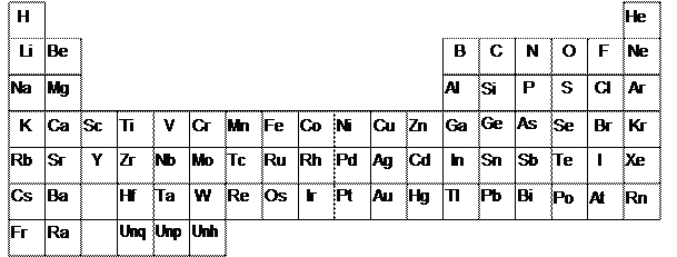


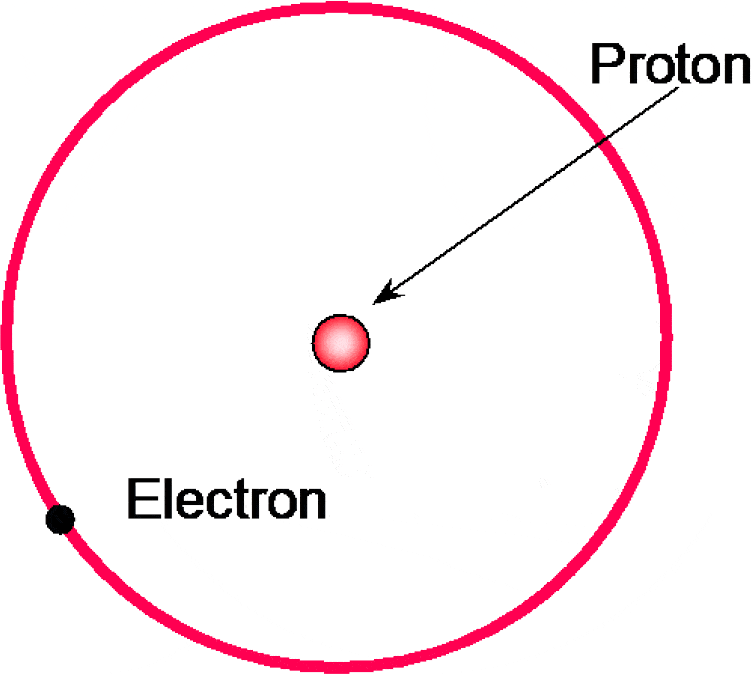


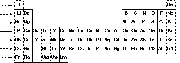


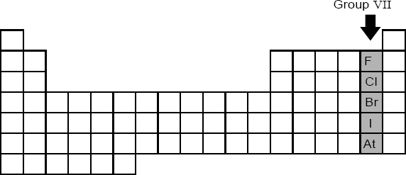
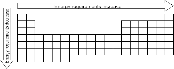

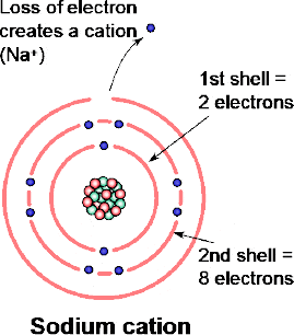

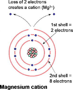


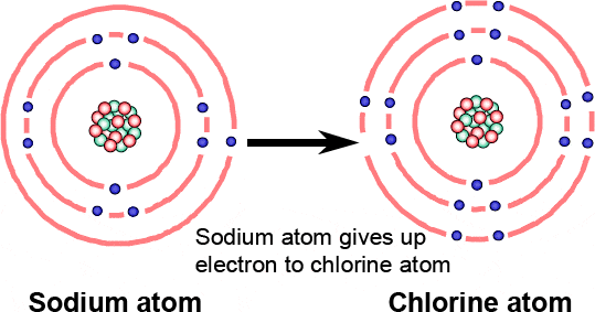


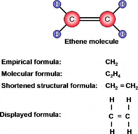
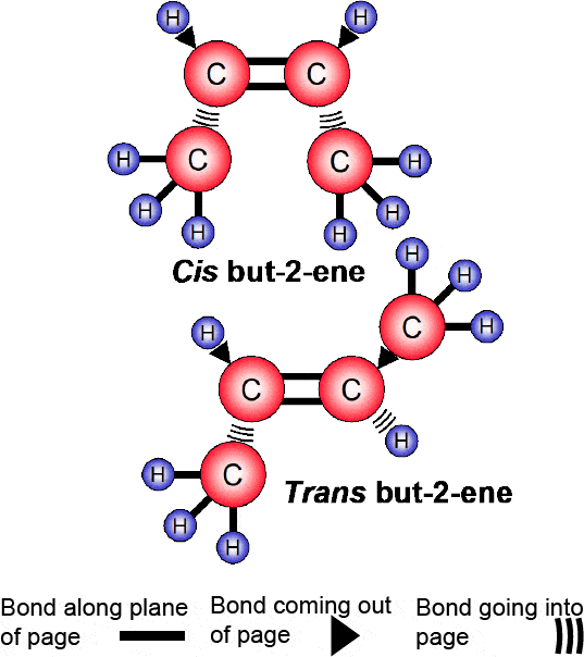
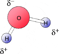


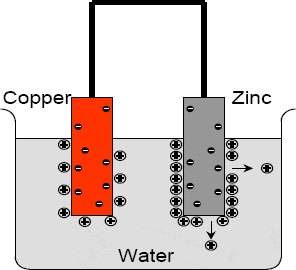

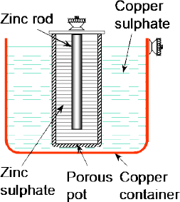
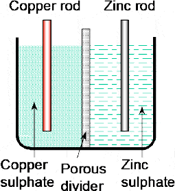

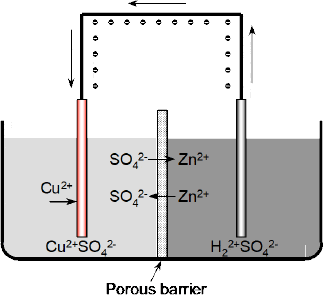

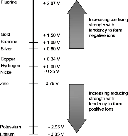
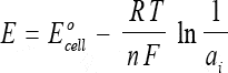


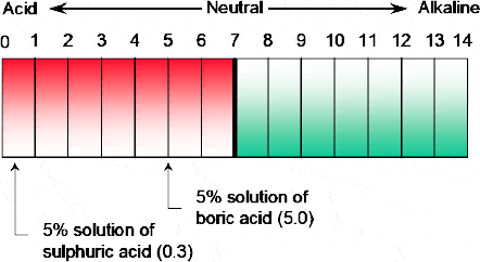


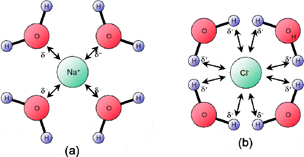


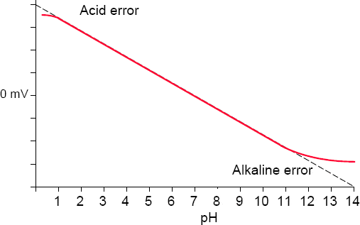
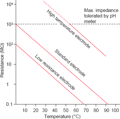
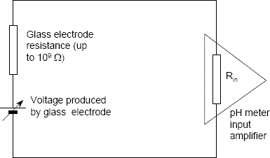


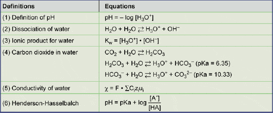
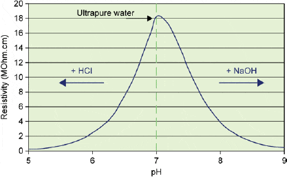


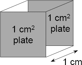


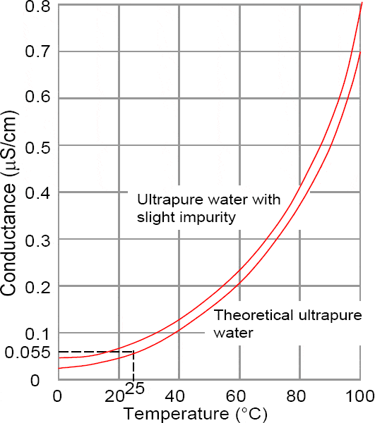


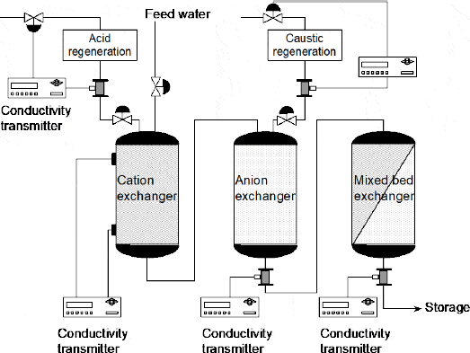
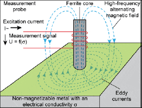
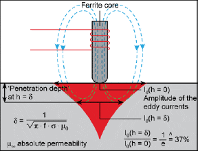


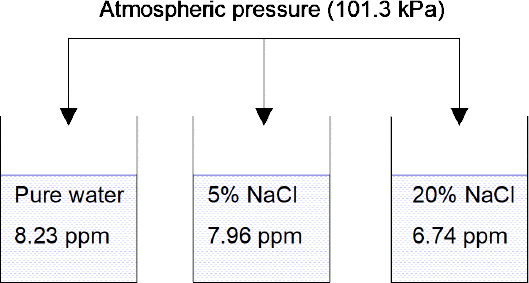

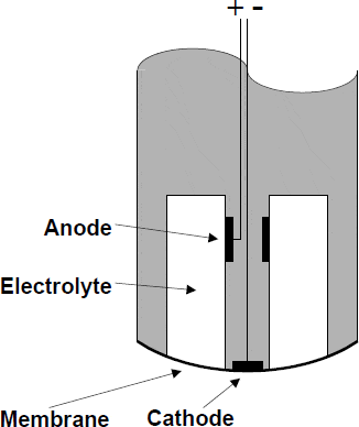


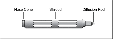

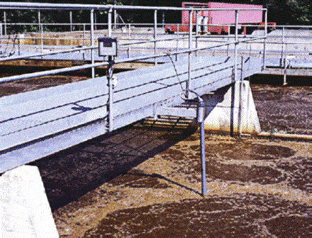


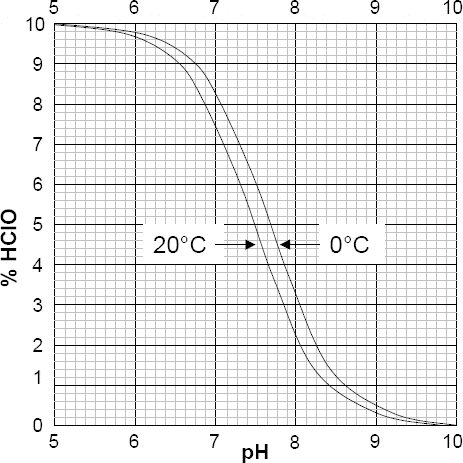


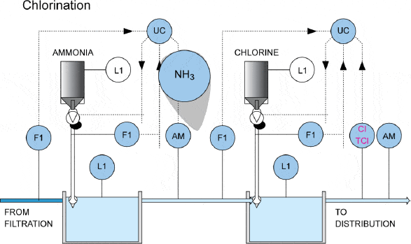

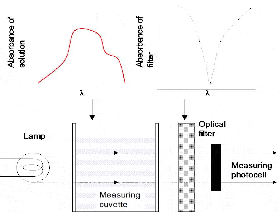


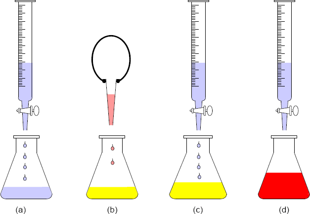


 button, to confirm this. Press the same button to take this away.
 button, to confirm this. Press the same button to take this away.
 button, to confirm this. Press the same button to take this away.
 button, to confirm this. Press the same button to take this away.
 button, to confirm this. Press the same button to take this away.
 and
and  buttons, to see what happens on both sides of the cell.


 button, and type in a value of 0.00010 moles / L (which, by the way, would be 0.10 moles / cm3).
 and observe the intensity of the light.


 and select the option that has
  as the Oxidizing agent and
  as the reducing agent.
 button.)


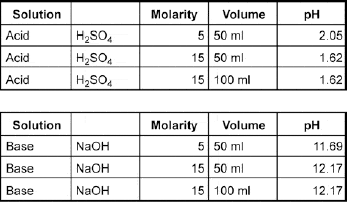

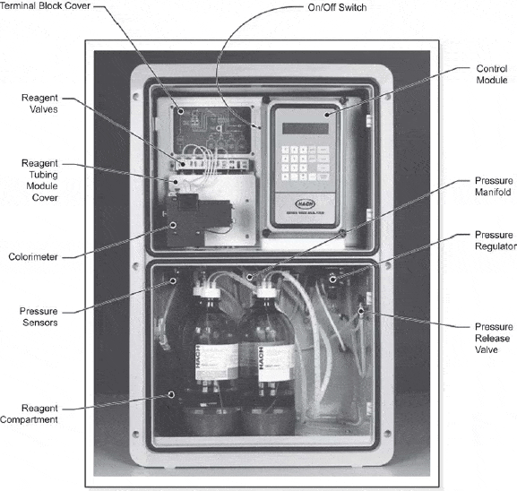


")


")


 & SCADA Systems")


")
")


")
