")
52896WA Advanced Diploma of Civil and Structural Engineering (Materials Testing)
Investigation of the properties of construction materials, the principles which…Read more")
Graduate Diploma of Engineering (Safety, Risk and Reliability)
The Graduate Diploma of Engineering (Safety, Risk and Reliability) program…Read more
Professional Certificate of Competency in Fundamentals of Electric Vehicles
Learn the fundamentals of building an electric vehicle, the components…Read more
Professional Certificate of Competency in 5G Technology and Services Overview
Learn 5G network applications and uses, network overview and new…Read more
Professional Certificate of Competency in Clean Fuel Technology - Ultra Low Sulphur Fuels
Learn the fundamentals of Clean Fuel Technology - Ultra Low…Read more
Professional Certificate of Competency in Battery Energy Storage and Applications
Through a scientific and practical approach, the Battery Energy Storage…Read more
52910WA Graduate Certificate in Hydrogen Engineering and Management
Hydrogen has become a significant player in energy production and…Read more
Professional Certificate of Competency in Hydrogen Powered Vehicles
This course is designed for engineers and professionals who are…Read more
This manual will provide you the basic knowledge of structural engineering including principles of analysis of structures and their application, behavior of materials under loading, selection of construction materials and design fundamentals for RCC and steel structures.
Structural Design for Non-Structural Engineers
Rev 9.1
Website: www.idc-online.com
E-mail: idc@idc-online.com
IDC Technologies Pty Ltd
PO Box 1093, West Perth, Western Australia 6872
Offices in Australia, New Zealand, Singapore, United Kingdom, Ireland, Malaysia, Poland, United States of America, Canada, South Africa and India
Copyright © IDC Technologies 2007. All rights reserved.
First published 2007.
All rights to this publication, associated software and workshop are reserved. No part of this publication may be reproduced, stored in a retrieval system or transmitted in any form or by any means electronic, mechanical, photocopying, recording or otherwise without the prior written permission of the publisher. All enquiries should be made to the publisher at the address above.
ISBN: 978-1-921007-24-8
Disclaimer
Whilst all reasonable care has been taken to ensure that the descriptions, opinions, programs, listings, software and diagrams are accurate and workable, IDC Technologies do not accept any legal responsibility or liability to any person, organization or other entity for any direct loss, consequential loss or damage, however caused, that may be suffered as a result of the use of this publication or the associated workshop and software.
In case of any uncertainty, we recommend that you contact IDC Technologies for clarification or assistance.
Trademarks
All terms used in this publication that are believed to be registered trademarks or trademarks are listed below:
Acknowledgements
IDC Technologies expresses its sincere thanks to all those engineers and technicians on our training workshops who freely made available their expertise in preparing this manual.
Contents
Preface iv
1 Structural engineering – an introduction 1
1.1 Introduction 1
1.2 Structural design – the process 3
1.3 Elements of structural design 4
1.4 Course objectives 5
1.5 Course outcomes 5
2 Structural systems & analysis of statically determinate structures 7
2.1 Classification of structures 8
2.2 Types of loads 11
2.3 Types of stress in structural members 15
2.4 Types of supports in structures 16
2.5 Equilibrium of bodies 17
2.6 Deformation of structures under loading 21
2.7 Structural classification based on degree of indeterminacy 23
2.8 Bending moment and shear force 27
2.9 Effect of moving loads 36
2.10 Analysis of pin-jointed frames 38
2.11 Influence lines 43
2.12 Conclusion 48
3 Principles of the Strength of Materials 49
3.1 Mechanical properties of the materials 49
3.2 Elasticity of the materials 49
3.3 Development of internal stresses 54
3.4 Flexural stresses in beams 56
3.5 Shear force and bending moment – the relationship 66
3.6 Bending shear stress 68
3.7 Horizontal and vertical shear – relationship 69
3.8 Bending shear stress – determination 70
3.9 Deformation of beams 75
3.10 The case of combined stresses 90
3.11 Analysis of columns 94
3.12 Conclusion 100
4 Analysis of Statically Indeterminate Structures 101
4.1 Structural classification based on the degree of indeterminacy 101
4.2 Principle of superposition 106
4.3 Analysis of statically indeterminate beams 107
4.4 Multi span or continuous beams 114
4.5 Slope deflection method 123
4.6 Moment distribution method 140
4.7 Influence line diagram for statically indeterminate structures 156
4.8 Conclusion 161
5 Design Theories 163
5.1 Stress-strain relationship for different materials 163
5.2 Design philosophies 166
5.3 Combination of loads 171
5.4 Theories of failure 172
5.5 Conclusion 172
6 Design of Steel Structures 173
6.1 Design of structures 173
6.2 Use of steel for structures 174
6.3 Properties of structural steel 176
6.4 Steel structural sections 177
6.5 Design of steel structures 178
6.6 Design of joints and fasteners for steel structures 179
6.7 Design of tension members 201
6.8 Design of compression members 207
6.9 Design of beams 219
6.10 Design of truss and allied structures 230
6.11 Conclusion 231
7 Design of Reinforced Cement Concrete Structures 233
7.1 Concrete – the material 233
7.2 Principle of reinforced concrete design 245
7.3 Design norms for reinforced concrete beams 258
7.4 Design of reinforced concrete slab 263
7.5 Design of reinforced concrete foundations 271
7.6 Design of axially loaded columns 279
7.7 Pre-stressed concrete – an introduction 285
7.8 Multistoried structures 290
7.9 Conclusion 292
8 Limit State & Plastic Design 293
8.1 Limit state theory 293
8.2 Design philosophy 294
8.3 RCC design by limit state 295
8.4 Steel structural design – plastic theory 304
8.5 Conclusion 314
9 Design and Construction of Masonry and Timber Structures 315
9.1 Masonry structures 315
9.2 Design of masonry structures 319
9.3 Timber construction 322
9.4 Strength of timber 326
9.5 Design of timber structures 327
9.6 Conclusion 330
10 Exercises 331
Construction is the largest industry in the world and of course, anything that is constructed needs to be designed first. Structural Engineering deals with analysis and design aspects, the basic purpose of which is to ensure a safe, functional and economical structure. Throughout the designing process, the designer constantly interacts with specialists like architects, operational managers, etc. Once the design is finalized, the implementation requires the involvement of people to handle aspects such as statutory approvals, planning, quality assurance, material procurement, etc. The entire exercise can be undertaken in a highly coordinated way if everyone involved understands the ‘project language’, which is a combination of designs and specifications. To understand the language fully, it is necessary to appreciate the principles of structural analysis and design, and a book on this topic comes in handy here.
Reading this book will help you gain the basic knowledge of structural engineering that includes principles of analysis of structures and their application, behavior of materials under loading, selection of construction materials and design fundamentals for RCC and steel structures. The emphasis has been kept on the determination of the nature and amount of stress developed under loads, and the way structures offer resistance to it. Being the most widely used construction materials, RCC and steel have been covered in detail, though masonry and timber have been described briefly as well.
This manual is suitable for anyone associated with the construction industry. In view of the vastness of the sector, the following personnel would typically be able to gain immediate benefit out of the course.
- Building Inspectors
- Project Managers
- Construction Supervisors
- Municipal Officials
- Architects
- Quantity Surveyors
- Insurance Surveyors
- Concrete Technologists
- Reinforcement Detailers
- Structural Fabricators
- Building Maintenance Personnel
- Structural Rehabilitation Staff
It is expected that this book will enable you to:
- Fully understand the role of a structural engineer
- Comprehend the behavior of structural members under loading
- Understand the concept of stress functions like tension, compression, shear and bending
- Use the basic concepts for analysis of statically determinate and indeterminate structures
- Analyze deformation of members under loading
- Understand the significance of material properties in design
- Undertake basic design of reinforced cement concrete structures
- Undertake basic design of steel structures
- Undertake basic design of masonry and timber structural members
This chapter describes the basic objectives of the course and provides an insight into various aspects of structural engineering, including its scope and the fields of its application.
Learning objectives
After completing the study of this chapter, you will be able to:
- Understand the role of a structural engineer.
- Gain awareness of the processes governing structural engineering.
- Appreciate the overall objective of the course.
1.1 Introduction
Structural engineering is the branch of engineering that deals with the analysis and design of structures. For this purpose, a structure can be defined as an assembly of various physical components, combined in a way which makes them act together effectively against loading conditions. This process of assembling or combining various elements together is called construction.
At times it may be possible for a structure to have only a single element, but such simple cases usually are rare.
Bridges, buildings, transmission towers, trusses, water tanks, industrial sheds, etc., are some of the common types of structures that one frequently encounters in day-to-day life. Figures 1.1 to 1.4 on the following pages illustrate some structures under various classifications.

RCC Building – Under Construction

Bridge
Of the examples shown, building in Figure 1.1, bridge in Figure 1.2, and industrial shed in Figure 1.3 are those which one usually comes across more often, whereas concrete dome in Figure 1.4 is not so common to observe and can be termed as special-purpose structures. The detailed classification of the structure has been described under the Chapter 2 of the manual.
Steel-Framed Structure

RCC dome
1.2 Structural design – the process
The basic purpose of the design of any structure is to ensure that it remains safe as well as functional under the most severe conditions of uses during its lifespan. The designer is expected to achieve this in the most economical way by following scientific principles.
The overall design operation follows well-established set of processes. The functional planning takes into consideration the purpose for which the structure is being designed. It involves provision of areas and spaces including their interrelation, planning of utilities and services required, providing for special features for the structure, etc. This process enables finalization of shape and plans of the structure. These layout plans get refined further as more experts get involved, providing their inputs on specific issues. These layouts are extremely important since they enable the designer to select the optimum structural system as well as the construction materials.
Further to deciding layout plan and structural arrangement, the designer starts working out the structural details of the individual components. This process involves determining the prospective loads applicable on the structure. The loads on the structure can be classified under several categories. This aspect has been dealt in detail in the chapter 2 of this manual.
In modern times, however, the complexity involved in the design process has gone up due to the following reasons:
- Due to advancements in manufacturing processes, the variety of construction materials available has widened considerably in the past few years. The characteristics of materials are also improving rapidly. The challenge for designers to keep themselves abreast of these developments need not be emphasized.
- The rate of flow of information coming out of various studies and research works, be it on method of analyzing or on the behavior of materials, has increased substantially during recent years. The speed of their adoption within the engineering profession has also gone up. This means that designers are constantly updating themselves on new principles, philosophies, analysis tools, etc.
- Design tools, which include software programs too, are being refined and upgraded quite regularly.
With these technological advancements in the field of engineering, it is specialist structural engineers nowadays who handle the task of designing the structures. At the same time, the engineering applications are often interdisciplinary, involving the participation of several disciplines of engineering. Construction engineers have always been involved in the overall installation and maintenance of structures. In the case of buildings, the architect plans and decides on the features of the project. Therefore, it is imperative that construction engineers and architects have some basic knowledge of structural design and engineering in order to perform their functions effectively. For industrial structures, the end user is usually a manufacturing engineer. The awareness of the structure’s behavior and limitations can help him decide on safe operational practices. Building inspectors, surveyors, etc., can also benefit from the knowledge of principles of structural engineering.
1.3 Elements of structural design
An engineering design activity may be defined as the application of basic principles of science to ensure a safe, easy in practice and cost-effective solution for a situation. In accordance with it, the structural design exercise simultaneously applies the principles of the following streams of science:
- Mechanics
- Strength of materials
- Statistics
The principles of mechanics are applied to analyze the behavior of each and every component of the structure under specified loading conditions. For this purpose, the members are commonly assumed to be rigid bodies, thus ignoring any deformations caused by induced stress. The principles of mechanics help in establishing external load–reaction relationships for the structure and its members. It is useful in determining the best structural arrangement for a particular situation.
The strength of materials is the science of relationship between an externally applied load and its internal effect on the bodies. For this, the bodies are no longer assumed to be rigid and their deformations under stresses are focused on. The application of the science of strength of materials helps in mainly determining the probable characteristic of material and through this, the optimum construction material itself. Also obtained are the sectional properties of the members for a given structural system. In addition, these principles help in the determination of internal stresses for more complex structural systems.
Statistics as a tool helps the design engineer work out the probability of a particular loading event occurring during the lifespan of the structure. With the help of this information, the engineer can identify the worst expected loading condition on a particular structural system during its entire lifetime. This is the most important set of information sought for the design process. Besides, statistics helps in identifying the probable variation in the behavior of various construction materials, although the load conditions may remain similar. This information is useful to determine the allowance that needs to be considered towards the material characteristics in a given situation. The studies on construction materials, though, are almost always done independently with their results made available to the entire design fraternity that can apply them in the relevant situations. It is important to state that in the event of an uncommon design situation, it may become necessary for the design engineer or engineers to undertake this entire exercise prior to finalizing the design.
Information technology is a facilitator that helps maintain design databases that are useful during routine design as well as in situations when new design philosophies are being implemented. In addition, with the help of the information technology, one can undertake the conduction load simulations as well as modeling for the proposed structure, which can highlight certain behaviors as well as validate the assumptions made. This is useful to finalize the form of the structure. The information technology assists the designer in even finalizing the drawings and design documents.
1.4 Course objectives
The main objective of this course is to bring good awareness of structural engineering principles to those who have no formal training in the subject but are still involved with building industry in certain roles. Apart from providing fundamental knowledge, the course aims to impart reasonable degree of skill in solving analysis and design related problems in structural engineering.
1.5 Course outcomes
- Acquiring basic knowledge of the properties and behavior of engineering materials.
- Gaining the ability to analyze the stress state of members under tension, compression, shear, and bending.
- Acquiring the ability to analyze deformation of members under loading.
- Understanding concepts used for analyzing statically determinate and indeterminate structures.
- Understanding the basic design of reinforced cement concrete structures.
- Understanding the basic design of steel structures.
- Understanding the basic design of masonry and timber structural members.
This chapter introduces the reader to the basic classification of structures, loads and stresses. The chapter also describes the principles and procedures involved in the analysis process in general. The methods and tools used in the analysis of statically determinate structures have been described in detail.
Learning objectives
After completion of this chapter, you will be able to:
- Understand the various types of structural systems.
- Understand about the typical components of structure.
- Understand the different types of stresses and the way structural arrangements offer resistance to them.
- Understand the load classification and the nature of stresses and deformations that they can induce.
- Understand the principles of mechanics and their applications in structural analysis.
- Use the analytical tools to analyze the statically determinate structures.
The function of all structures is to withstand stresses due to self-loads and direct loads imposed upon them and restraints imposed on physical characteristics, such as changes in dimensions with changes in temperature. The steps involved in a typical design exercise are as follows:
- Study the loads and constraints in the situation.
- Propose a suitable structural system.
- Examine the overall stability of the structure.
- Calculate the internal forces and deformations of the members.
- Modify and fine-tune the dimensions of the members.
The portion of the procedure that deals with the examination of overall stability and calculation of internal forces, support reactions and deformations in members is called structural analysis.
2.1 Classification of structures
Structures can be classified on the following bases:
- Purpose: Structures can be defined by the purpose of their erection. Typical uses are buildings for habitation (shown in Figure 2.1), dams for water retention (shown in Figure 2.2), bridges, factories and industrial sheds (shown in Figure 2.3), chimneys for flue gas discharge, and many more.

Buildings for habitation

Dam for water retention

Industrial structure
- Shape and form: Structures can be described on the basis of their form and shape. Common forms are beams, columns, slabs, walls, footings, frames, trusses, etc. A footing, for instance, is a form of foundation. Column is a vertical load bearing member and beam is a horizontal load bearing structure. Frame is a combination of vertical and horizontal members rigidly attached together.
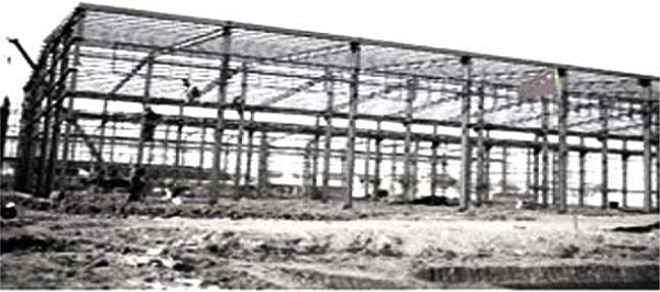
For illustration, a typical column–beam frame construction in steel is shown in Figure 2.4. One may also note the presence of inclined members, called bracing, about which we will learn in detail later on.

Column–beam construction in steel
- Analytical procedure: Structures are categorized by the procedure used for their analysis for subsequent design. Examples of such categorization are statically determinate and indeterminate structures, and two- and three-dimensional structures, respectively. The first set classifies the structure by way of complexity involved in their analysis. The second categorization is in accordance with the structure being confined within a single plane or its spread over a space, since the process of analysis changes accordingly. The photograph of a three-dimensional dome-shaped steel frame is in Figure 2.5.

Dome-shaped frame
- Material of construction: Structures are categorized based on the material used for their erection. The common construction materials are concrete, steel, masonry, and timber. Aluminum, glass, etc., are the ancillary materials used to feature the buildings, though they most of the time do not serve any structural purpose.
Typical brick and timber buildings have been illustrated in the photographs in Figure 2.6 and Figure 2.7 respectively.

Brick masonry building

Timber building
- Significance: The structure can be categorized as temporary and permanent, or primary and secondary, based on the importance they have in the overall scheme.
After classification system, we will now look at the kinds of loads which act on the structures. Further to it, the readers will be introduced to the fundamentals of structural analysis. The scope of this chapter is limited to the analysis of statically determinate structures. The analysis of statically indeterminate structures requires further understanding of the behavior of materials and, therefore, we will visit it after going through the section on ‘Principles of the strength of materials’.
2.2 Types of loads
As stated earlier, the structures are needed to withstand stresses developed due to loads imposed on them. To achieve this, it is essential to accurately assess all the loads that are likely to be imposed on the structure during its lifetime. It is also crucial to assess the possible combinations in which such loading events are likely to occur. The major types of loads applied to structures have been described below.
2.2.1 Dead loads
The dead loads are the self-weight of the structure and the weight of the permanent fixtures on the structure. The self-weight includes weight of the individual structural members and depends on their overall dimensions and the material of construction. Since the section of the member is derived based on the overall load application which itself is a function of the sizes being adopted, the process of initial determination of dead weight of structural members is somewhat iterative. For this, suitable assumptions about the components sizes are made in the beginning and are verified at the end, with the derived sections. Any correction can be incorporated at that stage.
Besides weight of the bare members, the dead weight takes into account permanent finishing like plaster, floorings, partitions, etc. The weight of all permanent installations, too, is considered within the dead load category. The data pertaining to the unit weight of the construction materials or the weight of the installations are obtained from the design codes and the manufacture’s specifications.
2.2.2 Live loads
The live loads, or the imposed loads, are the weight of its habitants, stored materials, temporary fixtures or movable equipment. The prominent difference between dead load and live load is that the former remains fixed but the latter is variable during the use of the structure. The live loads may also change their point of application that needs to be accounted while in the process of design.
The live loads on a structure can be classified into the following main categories.
- Weight of movable furniture and partitions
- Weight of occupants of the building
- Loads due to impact and vibrations
- Weight of movable equipments and fixtures
Most of the counties across the world have adopted certain standard values of live loads applicable on floors, roofs and other elements of the buildings. These standard values are related to factors like nature of building, occupancy, floor location, accessibility, etc. These live loads are expressed as uniformly distributed loads (UDL) over the area of application. Any dynamic or concentrated load is considered over and above this. Besides individual countries, the International Organization of Standardization (ISO) has published the codes on imposed floor loads for various types of buildings.
2.2.3 Lateral loads
Lateral loads are mostly imposed by nature in the form of wind and earthquakes. However, in the case of retaining structures like tanks and soil retaining walls, lateral loads also occur due to the pressure imposed by the material retained. Such load can be calculated with the help of established scientific theories.
The wind and earthquake-induced loads do affect the taller structure more than low-rise structures and, therefore, are of extreme importance in the analysis of high-rise structures and buildings. Both of these loads are transient loads.
Wind load:
In the case of wind loads, the applicability depends on the geographical region, geometry of the structure, its proximity with other structures, etc. Relative to the surface of earth, the natural air remains in motion. The difference in solar and terrestrial radiations results in differences in temperatures, which gives rise to convection, both upwards or downwards. The high-speed wind usually blows horizontal to the ground. And, therefore, the term wind denotes almost always horizontal wind. Vertical winds are specifically identified as such. Weak winds (i.e., winds at low speeds in the range of 5 kmph to 15 kmph) are termed as breeze and strong winds (i.e., winds at a speed of about 60 kmph) are termed storms. It is the storm the effect of which needs to be factored while designing.
In addition to normal wind, there are sudden blasts of wind that may last for few seconds. These are called gusts and may also require consideration. These gusts cause an increase in air pressure, but their effect on the stability of the building may not be significant. Often, the gusts influence only parts of the building and the increased local pressures may be more than balanced by a momentary reduction in pressure elsewhere.
As the wind velocity increases with height, a gradient of wind pressure is developed over the structure. Other important factors that come into play are the effective frontal area, depth with respect to wind direction, angle of attack, etc. The potential effect due to wind is analyzed and derived after giving consideration to all these factors.
Earthquake load:
The earthquake or seismic loads (since they occur due to movement within sub-terrain strata) are important to consider if the location of the structure falls in the active seismic zone. Seismic areas are regions, which are geologically young and unstable and, therefore, have a likelihood of experiencing earthquakes. The earthquake shock causes the earth to move and the structure too vibrates consequently. The resultant effect can be resolved in three mutually perpendicular directions. The horizontal effect on structure is generally considerable compared to the vertical one. The earthquake causes effective acceleration. The ratio of this acceleration to the acceleration due to gravity (g) is known as the seismic coefficient, which is applied during the design process as additional load over the structure.
Based on the type and importance of the structure, that may be designed either for horizontal seismic forces or both horizontal seismic forces and vertical seismic forces. The seismic accelerations for the design may be arrived at, from seismic coefficient, which is defined as the ratio, of acceleration, due to earthquakes, and acceleration, due to gravity.
Hydrostatic load:
The hydrostatic or water pressure is crucial for those structures which either retain aqueous liquids or are in contact with the underground water table. The earth or soil pressure again is imposed on underground structures or the soil retaining arrangements.
The hydrostatic load acts on a horizontal surface in accordance with the distribution shown in Figure 2.8. As is obvious, the intensity of the pressure is highest at the bottommost point of the surface. Therefore, the deep water structures are exposed to high intensity of pressure and overall load.

Hydrostatic load
Earth or Soil load:
Like hydrostatic pressure, the earth pressure is the lateral force that acts on the structures those retain soil or has been exposed to soil. However, unlike hydrostatic pressure, the extent of soil pressure depends on the intrinsic physical properties of the soil like its unit weight, cohesion, angle of internal friction, etc—besides factors like extent of overburden, angle of overburden, etc.

Soil load
The earth pressure may be calculated with the help of established theories of soil mechanics. For instance, as illustrated for a granular sort of soil like sand, the distribution of pressure on the retaining surface would be distributed in a triangular way. In the case of a more cohesive soil like clay, the pressure as well as the distribution pattern changes considerably. In this example, the active pressure at the depth H would be

It must be noted that for the same system, the value of the earth pressure would go up substantially if the earth pressure turns passive from the active earlier.
In addition to the normal pressure due to soil, the retaining structure may be exposed to more loads under special circumstances. The structures that retain expansive soils like clay are subject to further lateral pressure when the soils expand under moisture movement.
2.2.4 Snow load
In cold zones, the weight of snow on the structure can be predominant. The load due to snow acts as a dead load over the structure. Its occurrence and magnitude depend upon climatic conditions of the area and the exposure of the structure, its shape and geometry of its components.
The snow load depends upon the latitude of the place and the atmospheric humidity. The snow load acts vertically and it is expressed in kN/M² of plan area of the building or structure. The actual load due to snow depends upon the shape of the roof and its capacity to retain the snow. When actual data for snow load are difficult to obtain, load due to snow may be assumed to be 25 N/M² per mm depth of snow over the plan area of the structure.
During analysis, it is a usual practice to assume that snow load and maximum wind load will not be acting simultaneously on the structure.
2.2.5 Thermal loads
Thermal loads (or stresses) are generated because of inbuilt constraints that restrict the free expansion or contraction of structural members that otherwise would have taken place due to temperature variation. These loads are a function of the thermal property of the construction material used.
Variations in temperatures result in expansion and contraction of the structural members, while they are contained in the overall arrangement. This induces stresses within the members, which can be quite substantial at times. The range of variation in temperature varies from location to location and also from season to season. The temperature effects thus need to be accounted for properly and adequately. The combined value of stress developed because of design loads and due to temperature effects should not exceed the allowable limit. It is very important to take temperature stresses into account when the member is likely to face large variation in temperatures. The magnitude of thermal load is calculated as
| σ | = t x E x α | ||
| Where | |||
| t | = | change in temperature | |
| E | = | Young’s modulus | |
| α | = | Coefficient of expansion |
The coefficient of expansion is a physical property of the material and has different values for different materials.
2.2.6 Impact and vibrations
Dynamic or moving loads cause the impacts and vibrations on structures. The dynamic effects resulting from moving loads are accounted for by adopting an impact factor. The live load on the structure is computed in the normal way and the magnitude of live load is then increased by the impact factor. This takes care of development of additional stresses, due to the dynamic nature of the loads.
Vibrations can be an important factor while designing an industrial structure in which continuous vibrations of machines can cause severe stress in the supporting structures.
2.2.7 Erection and handling loads
Erection loads include all forces, to which a structure, or a part of a structure, is subjected during its transportation and/or erection. Erection loads also take into account the placement and storage of materials during the construction phase. Proper provisions should be made, for example, by providing additional reinforcement in the RCC, or temporary bracings in steel structures, to take care of all stresses caused during erection. The stresses developed because of handling and erection should never exceed the allowable values.
2.3 Types of stress in structural members
The loads imposed on a structure induce an internal reaction in a structural member which, when calculated per unit area, is called stress. A structural member or element normally is subjected to one or more of the following types of stresses.
- Tensile stress
- Compressive stress
- Bending stress
- Shear stress
The examples of these stress types are shown in Figure 2.10.
- Tensile stress: Direct tensile stress in a member is developed when a load system works to elongate the member along its axis. The failure generally takes place due to rupture. The member shown in Figure 2.10 (a) is subjected to tensile stress.
- Compressive stress: Direct compressive stress is developed when a load system works to reduce the overall length of the member. Thus in nature, it is opposite to tensile stress. The failure mechanism typically is slightly complex for such cases, and can be a combination of crushing and bending. The member shown in Figure 2.10 (b) is subjected to compressive stress.
- Bending stress: Bending stress in a member develops when a load system, acting either eccentric to the axis or normal to it, results in a moment at the section. This moment attempts to bend the member along some axis. The member shown in Figure 2.10 (c) is subjected to bending stress.

Types of stresses
- Shear stress: A system of forces whose result is a force acting perpendicular to the longitudinal axis of a structural member is called shear force. The stress developed due to shear force is the shear stress. It acts on a plane normal to the longitudinal axis of the member. The member shown in Figure 2.10 (d) is subjected to shear stress.
Apart from these situations, there can be an instance when the structure or its member is subjected to torsion stress due to the torque applicable at one end of the member. Such load applications, though, are not very common in the case of structures and, therefore, are not being elaborated on here.
2.4 Types of supports in structures
We will first consider two-dimensional structures where the members and the loads are located in a single plane. There are three kinds of supports for such a structure:
- Roller support: A roller support allows the rotation of a member about an axis perpendicular to the plane of the structure, as well as lateral displacement along the support by moving back and forth. It does not, however, allow vertical upward or downward displacement at the support location and therefore the only possible reaction is a vertical one (at the support location). The roller support is created by either using wheels at the end or having low-friction cylindrical rollers at the support. The schematic diagram of a roller support is shown in Figure 2.11 (a).
- Pinned support (also known as hinged support): This allows rotation of the member about an axis perpendicular to the plane of the structure, but restrains any movement or displacement of the member at the support location. Therefore, possible reactions are parallel to and perpendicular to the support base. The schematic diagram for this type of support is shown in Figure 2.11 (b).
- Fixed support: In this kind of support, the member is rigidly fixed to a base, which allows neither rotation of the structure nor displacement in any direction. Hence, as well as the reactions along and perpendicular to the support base, the fixed support can provide a moment as a reaction. The schematic diagram for this type of support is shown in Figure 2.11 (c).
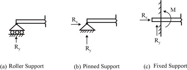
Types of supports
In the case of three-dimensional structures, also called space structures, the number of reactions for each kind of support differs compared to the same in the plane structures. Since the roller support would offer no resistance to rotation about any axis and also no resistance to the lateral displacement in any direction, the only possible reaction again will be a force perpendicular to the base. In the case of hinged supports, the rotation of the body in any plane is permitted but displacement is not permitted; hence the overall reaction is a maximum three linear forces acting along each of the axes passing through the support. In the case of fixed supports, the possible reactions are three forces along the axes and three moments about the axes passing through the support.
It must be remembered here that all the reactions described are those which can potentially be generated in a typical scenario. The actual generation of these reactions would depend upon the type of loading on the structure and the way in which the load pattern attempts to deform the structure.
2.5 Equilibrium of bodies
Let us consider the effect of loading on a body of random shape. Take a case where the body is subjected to a number of forces acting in different directions. If the body were stationary, it would be in the state of static equilibrium and if it were moving with a constant velocity (with respect to a reference), it would be in the state of dynamic equilibrium. In the case of structures, the state of static equilibrium is essential.
We therefore assume that the body does not change its state under the influence of applied external forces and is in the state of static equilibrium. As seen earlier (fixed support to a three-dimensional structure), a three-dimensional body has six possible motions. Three of them are displacements along the three axes and the other three are rotations about the same axes. Hence, six conditions have to be simultaneously satisfied for this body to be in the state of equilibrium. These conditions can be represented as:
- Σ Fx = 0
- Σ Fy = 0
- Σ Fz = 0
- Σ Mx = 0
- Σ My = 0
- Σ Mz = 0
These equations basically indicate that for the state of equilibrium, the algebraic sum of all the forces on the body along each of the co-ordinate axes and the algebraic sum of the moments due to these forces about these three axes should separately be zero.
In the case of two-dimensional or plane structures, the three corresponding representative conditions of equilibrium are as follows:
- Σ Fx = 0
- Σ Fy = 0
- Σ M = 0
2.5.1 Free-body diagram
When a body is in the state of static equilibrium, every part of it must also be in the same state. Therefore, if a cut is made at any place in the body and a part is isolated, that part must also be in equilibrium under the forces acting on it and the internal reactions at the section of cut.
A free-body diagram is a graphic representation of the body (i.e., a structure, an element of a structure or a piece of an element) with all of its connecting parts removed. Each one of these removed parts is replaced with external forces, which correspond to the internal forces present where that part connects with the body, such that the original state of equilibrium of the body is maintained. All the original loads on the body are also included in the force system.
All the required information to analyze and solve the structure under a force system is included in the ‘free-body diagram’. A ‘free-body diagram’ is a very useful tool to model the structure, structural element or sub-element that is under scrutiny. These diagrams may not be really necessary in relatively simple structural situations but have great utility when the structures become complex.
2.5.2 Preparation of a free-body diagram
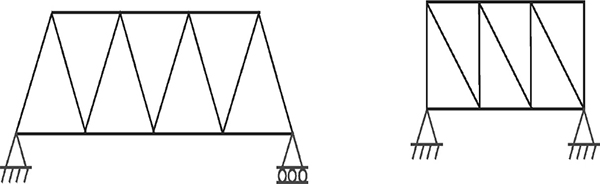
An example of how to prepare a free-body diagram has been illustrated below. We take the case of a beam AB of length l, supported at both ends on pin supports (which allow for rotation of the joint). The beam has been loaded at its center C with load W. The arrangement is shown in Figure 2.12.
At supports A and B, upward reaction forces RA and RB would act. It is clear that the sum of both these reactions is equal to the total load W.
Putting mathematically,
RA + RB = W
Taking the moment of all forces about support A,
W*(l/2) – RB*l = 0
From this, RB = W/2
Similarly, RA = W/2
We have decided to prepare a free-body diagram of the portion AD of the beam. For this, a cut is made at location D, which is at a distance x from the center, and the portion AD is separated from the system. Now, the forces acting on the isolated portion are as follows.
- Vertical external load W at point C
- Vertical reaction at support A, equivalent to

In addition, we have a moment at the end D of the free body MD and a shear force VD acting at D.

Preparation of free-body diagram
Applying the equations of equilibrium for the case:
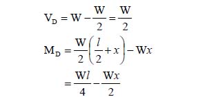
This demonstrates how useful a free-body diagram can be in the process of analysis of a structure.
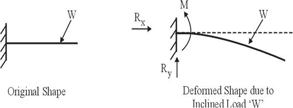
To make it clearer, the process for determining the reactions at the support of a cantilever beam with a concentrated load W acting at its free end is explained. The fixture at the wall is a rigid support for the beam, as it allows neither any rotation nor any displacement of the member. The arrangement is shown in Figure 2.13.

Free-body diagram for cantilever
The steps involved are as follows:
- First of all, one needs to draw a single-line diagram describing the system.
- Next, cut the beam free from the wall and replace the wall with the forces that were supporting the beam at the wall before it was cut free. The exact magnitude of these forces is not known at this stage but the nature is known, as they are acting in a way that keeps the beam in equilibrium.
- The internal forces in the beam before it was cut free from its support are determined when the forces that will keep the free-body diagram in equilibrium are found. The magnitude of the forces at the section cut will be identical to the internal forces in the beam at that point before it was cut.
A fixed support will resist translation in all directions as well as the rotation of the member. This will lead to the generation of corresponding restraining reactions that are consistent with the load system. In our situation, no lateral or horizontal force has been acting on the beam; therefore, there will be no horizontal reaction mobilized at the support. By applying the principles of equilibrium in the free-body figure above,
Σ Fx = 0
And, Σ Fy = W + V = 0; hence, V = (–) W
This indicates that the vertical reaction at the wall end will be equal in value to the load W but will act in the opposite direction. The load in combination with vertical reaction force causes a clockwise couple of value W×l that must be resisted by a moment at the end of the cut section acting in a counter-clockwise direction.
Again, applying the principle of equilibrium to obtain the value of this balancing moment,
Σ M = 0
Hence, balancing moment = (–) W×l
This explains the procedure of determining the internal forces within a structural element, with the help of a free-body diagram. To solve complex structures, a free-body diagram is prepared for each segment one after the other and the internal force determination is done in stages.
The same has been illustrated as below.
Illustration – 2.1: The beam shown in Figure 2.14 is simply supported at both the ends. We will draw the free-body diagram to determine reactions at both the supports.

Free-body diagram – illustration 2.1
In order to determine support reaction forces, the free-body diagram of the entire structural system has been drawn in Figure 2.8. For this, the supports at A and B have replaced with the upward reaction RA and RB respectively, balancing the downward load of 2T.
We know that moment at A is equivalent to zero. Hence,
MA = 0
On the other hand, from the free-body diagram,
MA = RB x 4 – 2 x 3
Therefore,
RB x 4 – 6 = 0
RB = 1.5kN
From the equilibrium condition Σ Fx = 0,
RA + RB – 2 = 0
RA + 1.5 – 2 = 0
RA = 0.5 kN
These derived values have been indicated in the free-body diagram, which has been drawn for the system.
2.6 Deformation of structures under loading
The application of loads on any structure leads to some deformation in the structure. The exact nature of the deformation depends on the nature of the load system, the overall arrangement of the structure, and the nature of the joints or supports.
Consider the joints or supports first. As described earlier, roller supports allow a member to rotate as well as permit lateral displacement in the plane of the joint. Thus, a member is free to rotate to a certain angle, as shown in Figure 2.15 (a), if it has a loading system consistent with this condition. Also possible will be the displacement at the joint in the plane of supports, but generally, the longitudinal displacement of the members along its axis is negligible and is ignored.

Types of deformation under loading
The deformation behavior in the case of hinged supports is similar to roller supports, except that no displacement at the supports is permitted. This is illustrated in Figure 2.15 (b), where it can be seen that a horizontal reaction RX develops in addition to the vertical reaction.
In the case of a fixed support, there is no scope for rotation or for the displacement of a member at the support. Hence in the case of transverse loading, as in the case of the beam in Figure 2.16, the end will not rotate and a tangent drawn at the point of support will lie along the axis of the beam only.
Deformation of a beam (fixed support)
The geometry of the system also influences the final deformed shape. For instance, in the case of the portal frame in Figure 2.17, the lateral force at joint (2) would be instrumental in the lateral displacement of joint (2) and joint (3) together. However, due to the rigid nature of the joints (2) and (3), the angle between the members connecting at these joints will remain unchanged and the tangents drawn at these points for the deformed members will always be at right angles.

Deformation of a portal frame under stress
Let’s consider the case of the portal frame in Figure 2.18, all the features of that are the same as the frame in Figure 2.15, except the introduction of a hinge support at joint (3).
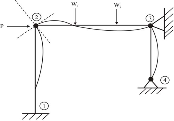
Portal frame and its deformed shape with constraint at point 3
Due to the introduction of this hinge, the lateral movements of joints (2) and (3) have been contained fully [ignoring the longitudinal deformation at (2)], despite being an unchanged loading system. The hinge support at (3) could also have been replaced with a force of magnitude equal to at P (2) to obtain similar results. This demonstrates the influence of the nature of the load system and overall structural arrangement on the deformation.
2.7 Structural classification based on degree of indeterminacy
We have read that structures can be classified as structurally determinate or non-determinate, based on the procedure of their analysis. We will further observe the characteristics that lead to this classification.
2.7.1 Statically determinate structures
Structures which can be completely analyzed with the help of statics alone are known as “statically determinate structures.” The process of finding the internal forces and reactions in these structures involves only the application of the equations of equilibrium. The process needs information on the overall arrangement of the members in the structure and the types of support constraints. At the same time the process is independent of all other geometric considerations, which means that the determination of internal and external forces and reactions can be done without giving any attention to the deformed shape of the structure.
To explain further, a determinate structure will have only as many supports as are absolutely essential for its stability under imposed loading conditions. Thus, a statically determinate structure can also be defined as the one in which the number of external forces and reactions equals the number of the equations of statics which are applicable for the particular situation.
2.7.2 Statically indeterminate structures
Those structures which cannot be fully analyzed with the help of statics alone are known as statically indeterminate structures. In these cases, the number of unknown reactions exceeds the number of applicable equilibrium equations.
Let us look at an example. Consider the case of a beam AB in Figure 2.19, which is fixed at end A and supported at end B. Structurally, this arrangement is known as a propped cantilever. An inclined load W has been imposed on the beam.
As is obvious from the diagram, there are four unknown support reactions: three at support A and one at support B. However, there are only three equations of statics (ΣH, ΣV and ΣM = 0) available; therefore, beam AB is a statically indeterminate structure.

Types of cantilevers
As we are aware by now, in the case of plane structures there can only be three possible equations of equilibrium. Does that mean that all structures with more than three unknown support reactions are statically indeterminate? Not necessarily. Consider a modification in the beam in Figure 2.19. Between A and B, a hinge has been installed at C. Clearly, the condition that the moment at C should be equal to zero provides an additional equation because the vertical reaction at B can now be found by considering the moment equilibrium of CB about C. With this additional equation, it has become possible to analyze all the four unknown reactions and, therefore, the structure has become statically determinate.
Let us consider another situation for beam AB. We decide to remove the support at B. The structure will still be stable under the influence of the load W. Simultaneously, it has become statically determinate even without the introduction of any hinge (in fact, in this situation, the introduction of a hinge would render it unstable). It can be concluded that the support B was redundant. We can therefore say that in a statically indeterminate structure, the number of support reactions is more than those necessary for the stability of the structure. This difference, or alternatively the number of redundant members in the structure, is known as the degree of indeterminacy of the structure.
2.7.3 Determination of degree of indeterminacy
As stated earlier, the degree of indeterminacy is the number of redundant support reactions in a structure, which, on removal, would make the structure statically determinate. Two popular methods to determine the degree of indeterminacy have been explained below. The scope has been confined to plane or two-dimensional structures only.
Cantilever tree method:
This method is useful for rigid jointed frames.
To work out the degree of determinacy for frames by this method, the first step is to ensure that all the joints be rigid ones. This is achieved by providing extra restraints at the non-rigid joints (to convert them into rigid ones). The number of such restraints is counted (R).
Now, the closed frame structure is cut in such a way that each isolated portion resembles a tree with branches on one or both sides. The numbers of cuts in the total structure are also counted (C).
Degree of Indeterminacy = 3×C – R
We will consider the example of the frame shown in Figure 2.20.

Cantilever tree method to determine the degree of indeterminacy
The frame in the example has two hinged supports. To convert them to rigid, each has had a single restraint applied.
| The total number of Restraints introduced ‘R’ | = 1 + 1 = 2 |
| The number of Cuts required to convert into tree ‘C’ = 6 | |
| Hence, degree of indeterminacy | = 3×6 – 2 = 16 |
The underlying principle can be applied to any structure to find its indeterminacy. In the case of indeterminate beams, what is required is to make any one end of the beam fixed (if it is not already) by introducing restraints. Once this has been done, remove all the redundant supports. The degree of indeterminacy can be worked out with the following relationship.
Degree of Indeterminacy = Supports Removed – Constraints Added
Method of joints:
This method is suitable for pin-jointed structures with a relatively large number of members. A truss is one example of a structure of this type. The principle applied is that each member of the structure has an unknown axial force, the number of which is added to the total number of support reactions. Now, each of the pin-joints contributes two of equilibrium equations. Therefore in the case of a plane structure:
| Degree of Indeterminacy | = Total Members + Total Support Reactions – (2 × Number of Joints) |

Statically determinate truss
Let us take the truss shown in Figure 2.21 as an example for illustration. The truss has a total of 13 members and 8 joints. There are two supports: a hinge and a roller. Total support reactions will be three in number (two for a hinge and one for a roller support).
Degree of Indeterminacy = 13 + 3 – 2×8 = 0
The zero degree of indeterminacy indicates that the truss is statically determinate. It may be noted here that if the roller support is converted into a hinged one, the total number of support reactions will increase by one; hence, the degree of indeterminacy will become one and the truss will no longer remain statically determinate.
2.8 Bending moment and shear force
We will consider the case of a traversely loaded structure or member, which has small lateral dimensions compared to its length. The axial loads acting on this member are either nil or negligible. These structural members are called beams. When a set of transverse forces acts on this structural member, they induce bending in its longitudinal axis. In order to resist this bending, a resisting moment is mobilized within the beam at any section. This moment is known as the bending moment. This is a crucial phenomenon for the analysis of traversely loaded component of structures like beams, slabs and beam columns. We will concentrate on the case of beams for this section.
Take the example of a beam AB supported at its ends and carrying the concentrated load W. The beam is held in equilibrium by the two reactions at its end, Ra and Rb respectively. For this case, we will consider the self-weight of the beam as negligible. We assume that the entire structural arrangement has been cut along section X-X. This divides the beam into two elements. The structural arrangement and free-body diagram of the left-side element are shown in Figure 2.22.

Structural arrangement and free-body diagrams of traverse-loaded structures
The free-body diagram of the left element shows that the support reaction, Ra, is the only vertical force acting. It is obvious that to maintain the equilibrium of the element, it is essential that the fibers in the exploratory section X-X must supply the resisting force required to satisfy the condition of equilibrium. Since both the external loads and support reactions are only vertical, the condition Σ Fx = 0 is automatically satisfied.
Now, to apply the other equilibrium condition Σ Fy = 0, the imbalance caused due to reaction Ra requires the fibers to mobilize a resisting force. This force Vx, as shown in the free-body diagram, would work along the section of cut and would work in the downward direction in this case. This force Vx is called the resisting shearing force. Also, the numerical value of V will be equal to Ra in this case. However, if the loading system is modified and a new load is introduced between Ra and section X-X, the value of Vx would change and would not remain equal to Ra. In this situation, the value of Vx will be equal to the net vertical imbalance to satisfy the condition of equilibrium.
Hence, it can be stated that the shear force at a section is equal to the total lateral force imbalance on either side of the section. The resisting shear will be equal in magnitude to the shear force acting on that section.
For complete stability of the left-side segment of Figure 2.22, the condition Σ M = 0 needs to be satisfied. In this case, Ra and Vx are equal and opposite forces. They produce a couple of value M, equal to Ral, which is called the bending moment, since it tries to bend the beam. The fibers in the section X-X are again required to mobilize a resisting moment of the same magnitude, indicated as Mx in the diagram.
In day-to-day working with structures, one comes across free bodies having a number of forces acting besides the reaction force. In situations of this sort where no single couple can be found working, the bending moment is defined as the algebraic sum of the moments about the lateral axis at a section, of all the loads acting on either side of the section.
2.8.1 Sign for bending moment and shear force
Normally, the bending moment which tends to produce the bending of the beam concave upwards is termed a positive bending moment and opposite to it, i.e. concave downwards, is denoted as negative. In the case of shear force, the force that tends to move the left segment upwards with respect to the right is considered a positive shear force. Similarly, the force that tends to do the opposite is termed a negative shear force. These sign conventions are shown in Figure 2.23.

Sheer force and bending moment – signs
2.8.2 Bending moment – influencing factors
In common structural problems, the quantum of the bending moment (BM) generated, including its nature, depends upon the following.
- Nature of loading
- Nature of supports
- Geometry of the structure
The nature of traverse loading is crucial for the distribution of the bending moment along the overall span of the beam. A load application can be of several types. A concentrated load or point load is the one that acts on a very small area compared to its intensity, and can be considered to be acting at a point. On the other hand, distributed loads have a larger area of application and are considered to be acting on a considerable length of the structure. Distributed loads can have several patterns of distribution. A uniformly distributed load is one that has even distribution of load along the length of the application. The uniformly varying or triangularly distributed load is the pattern where the application of the load increases at a constant rate. There can also be a non-uniformly distributed load. All these loading conditions are shown in Figure 2.24. It may be worth mentioning that in a large number of cases, the actual patterns encountered are non-uniformly distributed but from the point of view of ease in analysis, they are considered to be either uniformly distributed or uniformly varying patterns of loading.
The loading pattern on the structure affects the development of bending moment in a major way.

Types of distributed loads
Loads can be further classified as stationary or moving, as we will see later on.
The type of supports and overall geometry of the structural system also have a major influence upon the amount and distribution pattern of the bending moment and shear force. Two situations of beams having different spans (hence geometry), loading situations and support locations have been analyzed below.
To understand the concept of bending moment and shear force development clearly, we will consider a couple of situations and observe the process of determination.
Illustration – 2.2: A 4 m span cantilever beam has a single concentrated load of 4 kN working at a point 3 m away from the fixed end. There has been no other load over the beam. Find the value of the bending moment at the support.
As we know, a cantilever is a beam that has one end fixed and other free. The fixed end is rigid and prevents any rotation.
If we consider the forces for equilibrium, the only external load is 4 kN that is acting downwards. The only reaction possible is at support and, for the sake of equilibrium, that would be equivalent to 4 kN, acting upwards.
Considering section at the support, since the reaction does pass through it, the moment would be equivalent to the product of only load and the distance from the support.
M = 4 kN x 3m
= 12 kNm
Therefore, the value of the bending moment at support will be 12 kNm. As it is obvious that the beam will curve concave downwards, the sign of bending moment will be negative.
Illustration – 2.3: A simply supported beam, shown in Figure 2.25, is subjected to single-point load as indicated. We will draw the bending moment and shear force diagram for the entire span.
The first step is to determine the reactions at both the supports.
For this, let us use the equilibrium condition Σ MA = 0.
| 10×3 – RB × 5 | = | 0 |
| 30 – 5RB | = | 0 |
| RB = | 6kN |

Bending moment and shear force – illustration 2.3
Now, in order to determine the reaction force at A, we will use the equilibrium condition Σ FY = 0:
| RA + RB – 10 | = | 0 |
| RA + 6 – 10 = | 0 | |
| RA = | 4kN |
With RA and RB known, we can proceed to draw the bending moment and shear force diagrams in the following way. Since the bending moment at a section has been defined as the algebraic sum of the moment due to all the load on either side of the section and the shear force has been defined as the net imbalance in the lateral load on either side of the section, we have to use these definitions by converting them into mathematical expressions, to work out the value of the bending moment and shear force.
First of all, consider a section C on the span, located between point A and the 10kN load, spaced x from A. As per definition, moment at this section,
MC = RA*x
MC = 4x
As is obvious from the expression, the relationship between bending moment and the distance from the support is linear.
| For x = 0, | MC | = | 0 | |||
| For x = 3 (right near the load), | MC | = | 4*3 | = | 12 kNm | |
Now, consider another section D on the span, located between B and the 10kN load, spaced y from B. As per definition, moment at this section,
MD = RB*y
MD = 6y
As is obvious from the expression, the relationship between bending moment and the distance from the support is linear.
| For y = 0, | MD | = | 0 | |||
| For x = 2 (right near the load), | MD | = | 6*2 | = | 12 kNm | |
Resultant bending moment diagram is shown in Figure 2.19.
To draw shear force diagram, we will treat the entire span as two sections: first one, A to the 10 kN load and the second one as B to 10 kN load.
In the first section, the single vertical force acting between A and just left of the load is the reaction measuring 4 kN, irrespective of the location. Therefore, the shear force all along this segment would be 4 kN. Since the tendency would be to move the left segment upward with respect to right one, the sign of shear force is positive.
In the second section, the single vertical force acting between B and just right of the load is the reaction measuring 6 kN, again irrespective of the location. Therefore, the shear force all along this segment would be 6 kN. As the tendency now would be to move the right segment upward with respect to the left one, the sign of shear force is negative.
The section of the span subjected to downward load of 10 kN is the one where shear force changes its sign.
The shear force diagram is shown in Figure 2.25.
Illustration – 2.4: The objective is to draw the bending moment and shear force diagram for the beam shown in Figure 2.26.
The beam in the example is simply supported at both ends. We will start by computing the reactions at the support. For this, use the equilibrium equation Σ MA = 0:
50×5 + 5×10(15 +2.5) – RB × 20 = 0
Hence,
RB = 56.25 kN
Now, by applying the equation Σ FY= 0,
RA – 50 – 5×10 + 56.25 = 0
Hence,
RA = 43.75 kN
Now, with RA and RB known, we will consider three sections along the span of the beam AB to derive the values of the bending moment and shear force along the entire span. The first one is at location X at a distance of x m from B, the second one at Y at a distance of y m from C and the third one at Z at a distance of z m from A.
Consider the section at X first. Again, as the bending moment at a section has been defined as the algebraic sum of the moment due to all the load on either side of the section and the shear force has been defined as the net imbalance in the lateral load on either side of the section, we will use these definitions to work out the value of the bending moment and shear force.
Consider segment AZ first. The loads acting on this segment have are in the diagram.
MZ = RAz = 43.75z
It is clear from the equation that the relationship between Mz and z is a linear one.
For z = 0 (Section A), MA = 0
For z = 5 (Section C), MC = 218.75 kN.m
Hence, the bending moment varies from zero at A to 218.75 kN.m at C in a linear fashion.
Similarly, VZ = RA = 43.75 kN
Therefore, the value of the shear force along AC is constant independent of the location:
| VA = VC | = 43.75 kN |

Bending moment and shear force – illustration 2.4
Consider segment CY next and refer to the loads shown in this segment on the diagram:
My = RA (5 + y) – 50y
My = 43.75 (5 + y) – 50y = 218.75 – 6.25y
Again, the relationship between My and y has been found to be linear.
| For y = 0 (Section C), | Mc = 218.75 kN.m |
| For y = 10 (Section D), | Md = 156.25 kN.m |
Note that the values of Mc worked out previously and now are the same.
| Vy = 43.75 – 50 = (–) 6.25 kN | |
| Hence, | VC = VD = (–) 6.25 kN |
The value of shear force has been derived as a constant for the CD segment as well. However, notice the change in its sign. Also, the value of Vc derived earlier was 43.75 kN. The explanation for this is that due to the introduction of a point load at C, there has been an abrupt change in the value of the shear force. The value derived earlier is applicable to the segment on the left of C and the recent one is for the segment right of C.
Finally, we will consider segment BX, and watch the behavior of the bending moment and shear force along this portion of the beam. In the case of a uniformly distributed load, the total force from the block of the load is assumed to be acting at the centroid of the load block:

Mx = 56.25 x – 5x²
The above relationship between Mx and x is the equation of a parabola. Therefore, the bending moment diagram of a beam under the influence of uniformly distributed load will assume the shape of a parabola.
For x = 0 (Section B), MB = 0
For x = 5 (section D), MD = 156.25 kN.m
In the case of shear force,
Vx = 10x – RB
Vx = 10x – 56.25
i.e., under the influence of uniformly distributed load, the variation in the shear force along the span is a linear one.
For x = 0 (Section B), Vx = (–) 56.25 kN
For x = 5 (Section D), Vx = (–) 6.25 kN
The graphical representation of the distribution of the bending moment and shear force is shown in Figure 2.26.
Illustration – 2.5: A similar exercise of drawing the bending moment and shear force diagram for the beam is illustrated in Figure 2.27.
The beam is supported at A and B, with A being a hinged support and B a roller support. BC is a cantilever span of 3 m. The force at point C is acting at an angle of 45 degrees to the axis of the beam.
To determine the bending moment and shear force on the different sections, we will only visualize the states of the beam segments, instead of drawing them separately. This will speed up the process.
First of all, we need to determine the support reactions. In this case, the load at point C is inclined at 45 degrees to the axis of the beam. This has to be resolved into two components, along and perpendicular to the axis respectively.
The horizontal component = 20cos 45º = 14.14 kN
The vertical component = 20sin 45º = 14.14 kN
From the moment equilibrium about A,
30×6 – Rb9 + 14.14×12 = 0
Rb = 38.85 kN
From the vertical equilibrium,
Ra = 30 – 38.85 + 14.14 = 5.29 kN

Bending moment and shear force – illustration 2.5
The load at C has a horizontal component. Since only support A can offer resistance to the horizontal force, the entire horizontal reaction will be mobilized at A and will act along the centroidal axis of the beam.
| Horizontal reaction at A, Bending moment at D, |
Rax Md |
= 14.14 kN = Ra×6 = 5.29×6 |
= 31.74 kN.m |
| Shear force in the segment AD, Bending moment at B, |
Va Mb |
= Vd = Ra = (–) 14.14×3 |
= 5.29 kN = (–) 42.42 kN.m |
| Shear force in the segment DB, | Vb | = Vd = 5.29 – 30 | = (–) 24.71 kN |
| Bending moment at C, | Mc | = Zero (Free end) | |
| Shear force in the segment BC, | Vc | = 14.14 kN |
The bending moment and shear force diagrams are shown in Figure 2.25.
Note that the bending moment was defined as the algebraic sum of the moments about the lateral axis at a section, due to loads on either side of the section. Since the horizontal force and reaction are acting along the centroidal axis, there has been no bending effect due to the action of these forces.
2.8.3 Bending moment and shear force diagrams – notable features
We have drawn the bending moment and shear force diagrams for the two examples above. It is worth examining the profile of the bending moment and shear force diagrams and their interrelation. In the case of the shear force diagram, the abrupt change in the shear force at a concentrated vertical load is represented by a vertical line drawn to join the two values on either side of the loading.
The second observation is that in both examples, the bending moment assumes the highest positive or negative value at the section where either the shear force is zero or reversal in its sign takes place.
We will now observe its mathematical derivation. We have seen that the relation between the moment at a section Mx and its location along the X-axis, designated by x, has a mathematical relation.
Hence, Mx = f (x)
To find the value/values of x that maximize the bending moment, we know from calculus that Mx must be differentiated with respect to x and the result equated to zero. Solving this equation for x gives the points where the bending moment is maximized. However, we have seen from the example that the shear force is zero at this section. Therefore, dMx/dx must be the function for the shear force, V:
i.e., dMx = 0
dx
This relationship will be proved in the section on Strength of Materials. Therefore, it can be concluded that if the bending moment has a maximum value at a section along the span, the shear force at the section will become zero, and vice versa.
The third interesting feature, which is noticeable in the bending moment diagram of the second example, is the change in the sign of the bending moment at a certain section in the span. In this case, the section where reversal takes place is designated as I on the diagram. According to the sign convention for bending moment, a positive moment tries to deform the beam with concavity upward and the negative one with concavity downward. The reversal of the moment indicates that the shape of the curve is concave upwards in the segment AI and concave downwards in the segment IC. The point I, where the bending moment is zero, is called the point of inflexion (meaning no flexure) or point of contraflexure (meaning the direction of flexure changes)
2.9 Effect of moving loads
In situations so far it has been assumed that the loads on a beam, whether concentrated or distributed, are stationary and are imposed on specified points only. However, in actual practice, we come across situations where the loads are non-stationary, i.e., moving. A bus traveling on a bridge is one such example. The value of the axle loads due to the weight of the vehicle and passengers within can be considered as fixed, but the location of these loads over the span of the bridge will change. Hence, moving loads can be described as a set of loads when the value of each load and their positions with respect to each other are fixed, but the entire load arrangement can move.
2.9.1 Bending moment under moving loads
In the case of moving loads, it is critical to determine the specific location of the load set that causes the generation of the maximum bending moment at any section along the span.
For a set of concentrated loads, the maximum bending moment caused by the whole set occurs directly under one of the loads. Therefore, it is considered necessary to determine the values of the bending moments under each load, when the position of each load is positioned to cause maximum moment under it. The largest of these determined values will be the one governing the design of the beam.
In Figure 2.28, the case of a simply supported beam AB of span l is shown. The beam is subjected to a set of three loads W1, W2 and W3 acting at a distance of a and b from each other. These loads move as a set on the entire span of the beam and are free to occupy any location.
We will now show the example of locating position of the central load W2 when the bending moment under this load is the largest. Let us denote the resultant of this force system as W, acting at a distance of p from W2.
Applying the equilibrium equation:
Σ Mb = 0 = Ral – W(l – x – p)
Hence, 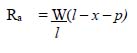
Now, the bending moment under W2 is


Moving loads on a beam
To obtain the value of x for which Mw2 is maximized, we differentiate the equation derived for Mw2 with respect to x and equate the value to zero:

This relationship determines the location of the load at which it would cause the maximum bending moment. It can be expressed in general form as follows.
In the case of a set of loads acting on a beam, the bending moment under a particular load will assume maximum value if the load occupies a location such that the center point of the beam is at equal distance from that individual load and the resultant of the entire load system.
2.9.2 Shear force under moving loads
Under the influence of moving loads, the maximum shear force will occur at one of the supports. There can be two situations of a load set for which shear force can be the maximum:
- When the extreme left load of the set is over the left support, the shear force on the left support will be the maximum.
- When the extreme right load of the set is over the right support, the shear force on the right support will be the maximum.
In the case of moving loads, the shear force is determined for both the conditions and the most severe value out of these is adopted for the design exercise.
2.10 Analysis of pin-jointed frames
Pin-jointed frames are multi-member structural systems, where each member is considered connected to the adjacent one through joints that act as hinges or pins. There will be situations where more than two members meet at a joint.

Truss- photograph
The most common example of a pin-jointed frame is the truss. A photograph of a truss is shown in Figure 2.29.
A truss is a structure made of many slender members. They are usually made of steel, but also of concrete and timber. In the case of steel trusses, the members are usually connected at the nodes or joints through the plate called a gusset plate. The members can be bolted, riveted or (most commonly) welded to the gusset plates. These connections are not ideal pin joints and their stiffness is taken into account in the design of the members carrying compressive forces, as we will see later.
Examples of pin-jointed frames (truss structures)
Trussed structures can be efficient for spans ranging from 2 m to even 30 m and (in some circumstances) more. The profiles of some typical truss structures are shown in Figure 2.30.
To analyze loads in the members of the truss, the following assumptions are made:
- As all the joints are pin joints, members will carry only axial forces (direct compression or direct tension).
- The application of external loads or reactions is only be at the nodes/joints.
- No lateral force will be applied on any member.
2.10.1 Statically determinate trusses
A truss for which the determination of all forces in the member, as well as the support reactions, can be done by applying the principles of statics is termed a statically determinate truss.
As we have seen earlier, in the case of a plane truss,
Degree of Indeterminacy = Total Members + Total Support Reactions – 2×Number of Joints
If a truss has a degree of indeterminacy greater than zero, the implication of this is that the truss either has (a) redundant member(s) or has more restraints at the supports than those absolutely essential from the point of view of stability.
If the degree of indeterminacy is less than one, the frame will probably be unstable under loads. There can be a situation where the configuration of the load system itself may provide stability to this type of frame, but inherently such a system is unacceptable. A system of this nature is called a mechanism.
In this section, we will observe the methods for force determination of members of statically determinate trusses. Two widely used analytical methods for this are:
- Method of joints
- Method of sections
Both use the principles of static equilibrium to find member forces. The method of joints is more appropriate when all member forces are to be determined and the method of sections is more suitable when only selected member forces are to be determined.
In this section, we will describe the method of joints.
2.10.2 Method of joints
In this case, each of the joints is analyzed separately by considering its equilibrium.
To explain the concept, consider the triangular pin-jointed truss shown in Figure 2.31. The load W has been applied at the crown C of the triangle. Node A has a hinge support and node B a roller support. For this truss,
| Number of Members | = 3 |
| Number of Support Reactions | = 2 +1 = 3 |
| Number of Nodes = 3 | |
| Degree of Indeterminacy | = 3 +3 –2×3 = 0 |
Therefore, the truss is statically determinate. To derive the vertical support reaction at B, we consider the moment equilibrium of the whole truss about A:

From the vertical equilibrium:
Ra + Rb = W. Hence, Ra =
Now, for the next step, we will consider node B in isolation and examine its stability under the influence of the forces acting on it. These forces are those in line with the longitudinal axes of the members AB and CB and the vertical reaction RB. We initially assume that the forces in the members are tensile. That is, they act on the body of joint B as shown in Figure 2.31.
Arrangement of a triangular frame
From the vertical equilibrium of joint B:

The negative sign coming from this equilibrium equation indicates that the assumed direction of force Pcb was incorrect and it is actually a compressive force.
Members in tension tend to pull their ends axially inwards and members in compression tend to push their ends axially outwards.
In the same way, if we consider the equilibrium of horizontal forces at node B, we get:

This is a tensile force.
The internal force in the member meeting at A can be determined in the same way. Considering the vertical equilibrium of A:
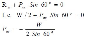
This force again is compressive in nature.
Similarly, considering the horizontal equilibrium at A:

Therefore, the horizontal component of the reaction at A is zero. Although the hinged support A has potential to mobilize horizontal reaction, in this case it has not happened due to symmetrical nature of the loading.
Illustration 2.6 – Using the method of joints, we will undertake the analysis of the truss shown in Figure 2.32, which has loads acting perpendicular to its top chord.
| In the truss under consideration, | |
| Number of members | = 9 |
| Number of nodes = 6 | |
| Number of support reactions | = 3 |
| Degree of Indeterminacy = 9 + 3 – 2×6 = 0, | |
| Hence the truss is structurally determinate. | |
Also, Length l12 = l23 = l35 = l56 = l25 = l45 = 2.1213 m
In order to derive the support reactions, we will consider the moment equilibrium of node 1 and node 6, one by one:
| Σ M1 | = R6×6 – 20×2.1213 = 0 |
| R6 | = 20×2.1213/6 = 7.071 kN |
| Σ M2 | = (R1V×6) – (20×2.1213) – 10×4.2426 = 0 |
| R1V | = (20×2.1213) + (10×4.2426)/6 = 14.142 kN |
To derive the horizontal reaction at node 1, equate the horizontal components of the external forces with the R1h,
R1H = 20cos 45º + 10cos 45º = 21.2132 kN
Now, to determine the forces in the members, we will consider the horizontal and vertical equilibrium of joints separately.
For Joint 6,
Σ Fx = 0, F65(sin 45º) = 7.071, F65 = 10 kN (C)
Σ Fy = 0, F 65(cos 45º) = F65, F64 = 7.071 kN (T)
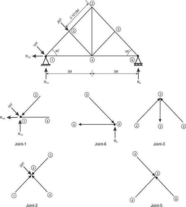
Analysis of a commonly used truss – illustration 2.6
For Joint 5,
There are three members that meet at this node. Out of these, two members – 56 and 53 – are in the same axis and the member 45 has its axis perpendicular to them. Now, it is obvious that the members 56 and 53 cannot have any force components perpendicular to their own axis. Hence there cannot be induction of force in the member 45 as otherwise joint 5 would not meet the equilibrium criteria. Therefore,
| F45 | = 0, | |||
| And for equilibrium, | F35 | = F56 | = 10 kN | (C) |
For Joint 3,
Σ Fx = 0, F32(cos 45º) = F35(cos 45º), F32 = 10 kN (C)
Σ Fy = 0, F34 = F32(sin 45º) + F35(sin 45º), F34 = 14.1421 kN (T)
For Joint 2,
Joint 2 has member configuration similar to Joint 5. The difference is in the presence of a 20 kN load, which has been acting along the axis of the member 24.
| Hence, | F24 = 20 kN | (C) | |
| And, | F23 = F21 = 10 kN | (C) |
For Joint 1,
| Σ Fx = 0, F14 = F12(cos 45º) + R1V –10(cos 45º) = 21.2132 kN | (T) |
All these member forces have been tabulated below. This table is useful to determine the required sectional properties of the member.
| Member | Force in kN | Nature of Force (Tensile = +ve, Compressive = –ve) |
| 12 | 10 | –ve |
| 32 | 10 | –ve |
| 24 | 20 | –ve |
| 34 | 14.1421 | +ve |
| 35 | 10 | –ve |
| 45 | 0 | — |
| 65 | 10 | –ve |
| 14 | 21.2132 | +ve |
| 64 | 7.071 | +ve |
2.11 Influence lines
An influence line can be defined as the graphical representation of the variation of a stress function at a point, when a unit concentrated load moves through the span of the structure.
A stress function is induced by the application of external force, for instance, bending moment, shear force, support-reaction, slope, deflection, etc. By drawing an influence line drawn for a section, it is possible at once to derive the value of the stress function at that section, for any specific location of the unit load.
The influence lines are useful in the following ways:
- With their help it is possible to find the positioning of loads that will lead to the maximum value of the stress function in a system.
- The value of any stress function can be determined under the conditions of critical loading.
For statically determinate structures, the influence lines for shear, bending moment and axial force will consist of straight line segment, as the relationship between these functions and the distance from the reference is always linear in the case of application of concentrated loads.
2.11.1 Influence lines for statically determinate beams
Consider the beam AB of span L, supported at both ends. The end A has a hinge support and B a roller support. It is subjected to a traverse load of unit value, which is moving along the span. At any instant, the load is at a distance cL from the end A. We will observe the variation in the bending moment and shear force at a section X along the span, which is located at a distance x from the support A. In addition, we will draw the influence lines for the support reactions. The entire structural arrangement is shown in Figure 2.33.
On the basis of equilibrium conditions,
| Reaction | Ra = 1 – c |
| Reaction | Rb = c |
| Shear Force at X | Vx = Ra = 1– c (if unit load is on the right of the X) |
| = – Rb = – c (if unit load is on the left of the X) | |
| Bending Moment at X | Mx= Ra(x) = (1 – c)x (if unit load is on the right of the X) |
| = Rb(l – x) = c(l – x) (if unit load is on the left of the X) | |
The value of ‘c’ varies from 0 to 1. As this variation in the value takes place, the resultant influence line diagrams for Ra, Rb, Vx and Mx are indicated in Figure 2.33. In a similar way, influence line diagrams for any statically determinate structure can be determined.
We will now observe the application of the influence line diagram for structural analysis. With the influence line diagram, it is possible to determine the value of the stress function for a given set of loading. We will take the case of a load system consisting of a number of concentrated loads P1, P2, P3, P4,……. working at points 1,2,3,4, … along the span. If the values of ordinates of the influence line at those sections are a1, a2, a3, a4,……. respectively, the total value of this stress function can be derived by just algebraically summing the products of the magnitude of forces with their respective ordinates. Hence, the overall value will be
= P1(a1) + P2(a2) + P3(a3) + P4(a4) + ……….

Influence lines for various stress-functions
In case the load is uniformly distributed instead of being concentrated, the influence line still can be used to determine the stress function. Suppose a load of intensity w per unit length is working on the span of the beam covering a length x from points X to X’ as shown in Figure 2.34. The influence line under consideration is for the support reaction Ra.
As shown in the diagram, the application of the load starts at X at a distance ‘a’ from end A and ends at X’ at a distance ‘b’ from A.
Hence, x = b – a

Influence lines- support reaction
As shown in the diagram, the load on a small element dx is w*dx. If the coordinate at the location is a1, the value of the support reaction at A,
= a1 (wdx)
The total reaction at support A due to the entire uniformly distributed load
| Ra | = ∫ a1 (wdx) |
| Ra | = w × Area of the portion of the influence line affected by the load. |
Illustration 2.7: The problem below will illustrate the procedure of drawing the influence line diagram and its application.
For the beam shown in Figure 2.35, we will draw the influence lines for the following:
- Support reaction at A
- Bending Moment at Section X, located 4 m from the end A
- Shear Force at section X
We will also work out the values of above stress functions, under the influence of a set of four concentrated loads, as shown in the diagram
Influence line for Ra:
The overall span of the beam is 10 m and the section X is located at a distance of 4 m from end A. The influence line diagram for Ra is a simple triangle as Ra will be equal to the unit when the unit load is right over A and equal to zero when the unit load is right over the support B. In the intermediate location, the variation will be linear.

Influence line diagrams- illustration 2.7
Influence line diagrams for Mx and Vx:
For drawing the influence line for Mx and Vx, we will consider the unit load acting at X. From the vertical equilibrium condition:
Ra = 0.6, and Rb = 0.4
| Hence, | Mx = 0.6×4 = 2.4 kN.m |
| And, | Vx = 0.4 kN on the left segment and (–) 0.6 kN on the right segment. |
The resultant influence line diagrams are shown in Figure 2.35.
For the locations of the concentrated loads of the load system, the ordinates of Influence Lime diagrams have been calculated and shown in the diagram.
From the diagrams,
Ra = (10×0.9) + (20×0.7) + (15×0.5) + (5×0.3) = 32 kN
Mx = (10×0.6) + (20×1.8) + (15×2.0) + (5×1.2) = 78 kN.m
Vx = (10×0.1) + (20×0.3) – (15×0.5) – (5×0.3) = (–) 2 kN
The accuracy of these results can easily be verified with the help of other analysis tools, which we have used earlier in the chapter. Influence lines are very convenient and useful for the structural analysis and are equally applicable for the statically indeterminate structures. The procedure is slightly complex in the case of statically indeterminate structures but there is availability of certain tools, Muller Breslau’s Principle for instance, which can make the procedure simpler. We will study the same in the Chapter 4 of this manual.
2.12 Conclusion
We have studied the various classifications of structures in this chapter and can appreciate the variation. We have also gained knowledge about the principles of statics and their use as tools for the analysis of statically determinate structures. Since the effectiveness of the design is dependent, to a large extent, on the accurate estimation of the loads on the structure, it is important to understand their types, effect and method of estimation. We have studied the effect of different types of loads on the structure. We also have understood the response of the structures to any type of loading, in terms of nature and magnitude of stresses induced in their different components. This knowledge about the structural behavior, in combination with the knowledge about the characteristics and behavior of material, is useful for undertaking the complete design of structures.
This chapter describes the physical behavior of materials from the engineering point of view. It explains the changes that take place within the material due to imposition of stress and also helps define their limiting conditions.
Learning objectives
After studying this chapter, one will be able to:
- Understand the mechanical properties of the material, important from a structural engineering point of view
- Understand the behavior of the material under stress
- Understand the mechanism of deformation of materials and evaluate the magnitude of this deformation
During the course of the selection of material for a structure or its component, it is vital to fully understand the behavior of a particular material under conditions of loading. The resistance to failure (strength) and the resistance to deformation (stiffness) of a structural member are the functions of the geometric properties of the member as well as the physical properties of the construction material. It is absolutely essential to understand and be familiar with these physical properties and also the limiting conditions of failure for the materials.
3.1 Mechanical properties of materials
The mechanical properties related to the strengths and deformations of materials are considered important from the point of view of structural engineering. In the case of most commonly used construction materials, the determination of various properties is done in laboratories. Specimens of materials are put under loads imposed with the help of machines that induce stress and strain of the desired nature and degree. The behavior of these specimens is observed under the stress conditions and the results are used to establish the permissible limits.
3.2 Elasticity of materials
While analyzing the structures and their components using the principles of statics, it is assumed that the structures are rigid bodies and do not undergo any deformation. This assumption helps simplify the process of analysis. However, the fact remains that all the material bodies undergo deformation when loads are applied to them. The magnitude of these deformations is different for different materials. When the applied load is removed, the body does overcome this deformation and assumes its original shape, provided the loading was not excessive beyond a certain point. This property of the material to regain its original shape when the load is removed is known as elasticity.
A material that regains its original size and shape on removal of stress is said to be an elastic material, while a material that undergoes permanent deformation without rupture is said to be a plastic material. A limit up to which a material shows perfectly elastic properties is known as the elastic limit.
The concept of elasticity is crucial, as experiments have established that a large number of materials exhibit elastic properties, albeit as long as the loading remains within certain limits.
3.2.1 Stress and strain
When a prismatic member has a load applied along its axis, the load is uniformly distributed along its entire cross-sectional area.

Member in direct tension
Again refer to Figure 3.1. Due to the application of the tensile force F on the bar, an increase in the overall length of the bar takes place. Since the end B of the bar is fixed, its other end B’ will shift to B” to accommodate this change. The change in the length of the bar B’B” is ΔL.
As shown in Figure 3.1, the prismatic bar BB’ of length L has had a tensile force of magnitude F applied along its axis. The cross-sectional area of the bar is A. On section XX’ of the bar,
Force per unit area = F/A = σ
This force per unit of sectional area is known as the stress. It is the internal force developed within the bar to resist its structural failure. As is obvious from the derivation, the unit of stress is kgfcm2 (N/mm2 in SI units).
Elongation per unit length of the bar  .
.
This elongation per unit length (contraction in the case of compressive force) is known as the strain. As the strain is the ratio of two quantities having similar units, it is just a number without any unit.
3.2.2 Hooke’s law and modulus of elasticity
‘Within elastic limits, stress is directly proportional to the strain.’
The statement above is known as Hooke’s law. It is a very important relationship between stress and strain and has wide application in the design of several mechanisms, apart from the design of structural members.
Hooke’s law, presented mathematically, can be stated as follows.
Within elastic limits, variation in stress is directly proportional to strain:
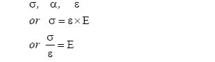
This constant E is known as the modulus of elasticity or Young’s modulus. Theoretically, it is the value of the magnitude of the stress required to be induced in a specimen of the material to increase its length to double the original length, provided the material remains in the elastic state throughout. The modulus of elasticity has different values for different materials, which invariably are very large. Since it is the ratio of stress to strain with strain being a unitless quantity, the unit of the modulus of elasticity is the same as that for stress, i.e., kg/cm2 (N/mm2 in SI units).
If we plot the strain of an elastic member against the corresponding value of stress within it, the resultant graph would be a straight line. The same is shown in Figure 3.2. The strain has been plotted on the X axis and the stress on the Y axis. It may be noted here that, by convention, strain is always plotted on X axis in a stress strain figure.

Typical stress strain figure for elastic bodies
The slope of the line OP in Figure 3.2 indicates the modulus of elasticity for the material.
3.2.3 Lateral strain and Poisson’s ratio
As is clear now, when a material is placed under tensile stress, a corresponding strain is generated along the direction of the stress, which increases the length of the specimen. It has been observed during studies that this elongation will always be accompanied by a contraction in the directions lateral to the stress. Within elastic limits, the ratio of these strains is constant for a material.
Lateral strain/axial strain = μ (constant)
This ratio μ is known as Poisson’s ratio for the material.
Theoretically, it has been calculated that the value for Poisson’s ratio for most materials should range between 0.25 and 0.33, while it should be 0.25 for an isotropic material. Isotropic materials are those having physical properties that do not vary with direction. Let’s try to examine the limiting value of Poisson’s ratio.
We will consider the case of a prismatic specimen of a material, for which the values of E and μ are known. Suppose the original length of the specimen is lo and the original cross-sectional area is Ao.
Hence, the original volume of the specimen Vo = Ao × lo.
The tensile stress of value T per unit area is applied on the specimen such that the material remains within the elastic limit and also follows Hooke’s law. The new length of the specimen is then
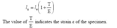
Corresponding to this increase in length, there will be some contraction in lateral directions. The effect of these contractions will be a reduced cross-sectional area for the specimen. With Poisson’s ratio for the material being μ, the new cross-sectional area will be
An = Ao (1– μ×ɛ)2
Hence, the new volume of the specimen will be
Vn = Ao(1– μ×ɛ)2 lo (1+ ɛ)
Since ɛ would be a very small value normally, we will ignore the value of its square from the expression.
It results in,
Vn= Aolo(1 + ɛ – 2 μɛ)
| The change in volume is | ΔV = Vn – Vo ΔV = Aolo (1 + ɛ – 2 μ×ɛ) – AoLo ΔV = Aolo(ɛ – 2 μɛ) = Aoloɛ(1 – 2 μ) |
The change in volume per unit of volume is
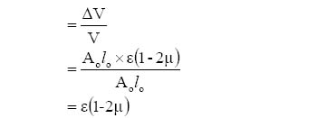
We can safely assume that the volume of any material will not reduce while under tension the value of the above expression will not become negative. To meet this condition, the limiting value of Poisson’s ratio can be 0.5, which denotes the unchanged volume during the process of deformation. In the case of metals, most of them exhibit a value of Poisson’s ratio between 0.25 and 0.35, which indicates some increase in the overall volume. Concrete, on the other hand, generally exhibits a value around 0.1.
With the knowledge of Young’s modulus and Poisson’s ratio, we understand two very important properties of matter from the point of view of structural engineering. The knowledge about Young’s modulus for materials helps in deriving the values of deformations in the structures under stress. Poisson’s ratio, on the other hand, helps in understanding the failure mechanism of various structural materials. Both these aspects will be elaborated on further as we move forward in the chapter.
3.3 Development of internal stresses
In the previous section, we have understood the development of stresses under direct or plain tensile, compressive and shear force. The phrase direct or plain must be taken note of here. This is the situation when the loads that are generating these stresses are either acting along the axis of the member, as in the case of tensile and compressive stresses, or are working normal to the axis, as in the case of shear stresses. In all these situations, each applied load is supposed to generate only a single type of stress, the value of which remains uniform along the entire cross section.
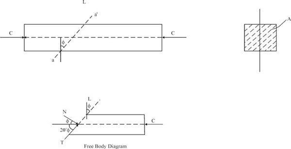
Stress on oblique section
Take for instance the case of a material specimen of length l and uniform cross-sectional area A, as shown in Figure 3.3. The specimen is subjected to a compressive force C along its longitudinal axis. Considering a cross section normal to the axis, the value of the applicable compressive stress will be equal to C/A = σ.
Now take the case of an oblique section a-a’, which is at an angle ϕ with the axis normal to the longitudinal axis of the specimen. What will be the nature and magnitude of stresses at this cross section? To evaluate, we isolate the portion of the specimen on the right of a-a’ and represent it as a free body.
This free body is then subjected to an external force C at the end and an internal reaction R takes place at the section. From the equilibrium condition, we have
C = R
The reaction R is acting at an oblique section. We resolve R into two components – one normal and the other tangential to this oblique section. From geometry, it is obvious that the angle between R and the normal component N is ϕ and the angle between R and tangential component T is (90 – ϕ).
Therefore, N = C cos ϕ
And, T = C sin ϕ
Area of the inclined section resisting these forces is 
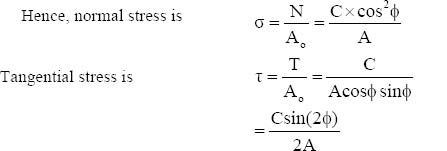
We have derived the expressions for normal and tangential (or shear) stress for a section, which is inclined to the axis of the member, when the member is subjected to a load along its longitudinal axis. We have considered the case when the load is compressive, but the expression is true for even the situation when the load is tensile. Only the direction of the stresses will be different in the case of a tensile force. It would be useful to observe the variation in these stresses with the variation in the angle of inclination.
When ϕ = 0,
σ = C/A, easy to understand as section will be normal to the axis of the member.
τ = zero, as the force along the axis cannot have a component perpendicular to itself.
When ϕ = 45º,
σ = C/2A
τ = C/2A
When ϕ = 90º,
σ = zero
τ = zero
Hence, the value of the normal stress has seen to be decrease from C/A at ϕ = 0 to half its original value when ϕ = 45º, and eventually to zero when the plane of the inclined section lies along the axis of the member.
The variation pattern of the shear stress is more interesting. Its value remains zero when ϕ = 0, reaches a maximum of  when ϕ = 45º, and goes back to zero when ϕ assumes the value of 90º.
As has been established that the maximum value of shear stress is reached at the section at 45º to the axis of the member and its magnitude is equal to half of the maximum normal or longitudinal stress, it is very important to understand the implication of this phenomenon. When a structural member is made of a material which has much lower strength in shear than in the tension or compression, the failure under axial load is more likely to take place due to slipping along a plane at 45º to the axis, and much less likely due to rupturing along the section normal to the axis. Even when the failure takes place due to slipping along an inclined plane, it is general practice to recognize it as a failure under compression or tension and the stress acting normal at failure is recognized as the ultimate tensile or compressive stress for the material.
A large number of construction materials have lower resistance to shear than to axial forces. As we will see ahead, even the failure of low carbon steel or mild steel is influenced by this phenomenon.
3.4 Flexural stresses in beams
The concept of bending moment and its derivation for a structure (statically determinate) has been studied in the previous section. Here, we will see the development of internal stresses due to the bending of members. These stresses are known as bending or flexural stresses.
To derive these stresses, we will study the behavior of the member under bending. The following assumptions are made when studying this behavior.
- The material of the member remains in linear elastic condition, i.e., obeys Hooke’s law.
- The plain section before bending remains plain after bending.
- The values for modulus of elasticity are the same for tension and compression.
- Each layer can enlarge and contract independently.
- The stresses are purely longitudinal and local effects of concentrated loads are neglected.
A simply supported beam AB is shown in Figure 3.4. Concentrated load W is acting at a point along the span. The reactions generated at both ends are Ra and Rb respectively. Due to application of force, the beam does deform and assumes a certain degree of curvature. We are considering here a case of pure bending, i.e., the section is free of shear force.
In the beam, two sections a-a’ and b-b’ exist normal to its axis and near each other, having a distance dx between them. Before the deformation of the beam, these sections are parallel to each other. Due to the effect of bending of the beam, both the sections a-a’ and b-b’ rotate to different degrees with respect to a datum. Let’s say that due to this unequal rotation, the angle between these is dθ. As we have assumed, the plane a-a’ and b-b’ would remain undistorted despite this rotation.
An enlarged view of the portion a-a’-b’-b after deformation is shown in Figure 3.4. Due to bending, the top fibre a-b shortens in lengths whereas the length of the bottom fibre a’-b’ increases. This variation in length, positive or negative, will be extreme for the outermost fibres and would keep on decreasing as one moves towards the center of the beam. Somewhere in the beam lies a fibre whose length remains unchanged during bending. The surface along which this fibre lies is known as the neutral surface. Resultant from the no-strain condition, the fibres along the neutral surface experience no stress.

Bending of beam under load
To determine the change in the length of fibres, a line c-c’ has been drawn in the diagram showing the enlarged portion of the segment a-a’-b’-b, which is parallel to a-a’. Hence, bc is the reduction in length of the topmost fibre and b’c’ is the enlargement of the bottommost fibre of the beam. Note that there has been no change in the length of the fibre along the neutral surface.
We consider the deformation of a fibre along a randomly selected layer. Suppose the layer is m-n and is located at a distance ‘y’ from the neutral surface. As the layer m-n is located in the elongation zone, its length has increased by a value of n-o resultant to bending.
Then, n-o = y(dθ)
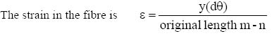
The length m-n is the original distance between the planes and its value will be equal to length d-e, since d-e lies on the neutral surface. If the radius of bending is denoted by r, the length d-e (and m-n too) will be equal to
d-e = m-n = r(dθ)
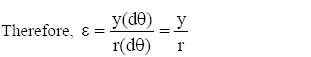
The objective is to evaluate the stress in the fibre. Since the material obeys Hooke’s law, the value of the stress in the fibre m-n is
σ = E(ɛ), where E is the modulus of elasticity for the material.

This expression indicates that the value of the stress in a fibre layer varies linearly and is directly proportional to its distance from the neutral surface.
The distribution of this stress about the neutral axis over the depth of the beam is shown in Figure 3.5. In this, the axis x-x’ is the neutral axis for the section, which is the cross section of the neutral surface and the normal section under consideration. The nature and therefore the direction of the stress are opposite to each other in the region above and below the neutral axis.
These stresses, distributed over the section of the beam member, must form a resisting couple M from the point of view of equilibrium.
As shown in Figure 3.5, an element of area dA of the cross section is located at a distance of y from the neutral axis.
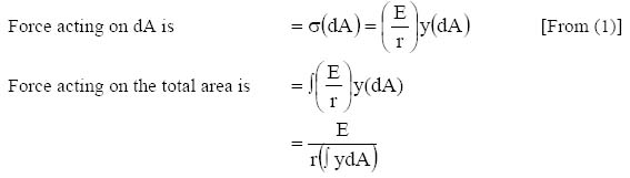
Since we are considering the case of pure bending and no other direct force has been applied on this section, the resultant of the forces acting on the cross section should be zero.

Since E in this expression cannot be equal to zero, the value of ∫y dA should be zero to satisfy the above condition.
Hence, ∫ y dA = A×yc = 0.

Stress development under bending
Again, since A is the overall area of the section and cannot be zero, the value of yc should be equal to zero.
yc is the distance of the centroid of the area from the neutral axis. Hence it can be said that the centroid of the area coincides with the neutral axis.
The moment of the force acting on area dA about the neutral axis is
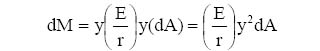
The total bending moment on the section will be the moment of all such forces over the cross-sectional area A of the section.
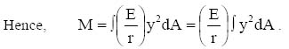
The expression ∫ y2dA is the sum of the multiplication of all the elements of the area with the square of its distance from the centroidal axis of the area. This expression is known as the moment of inertia of the section and is expressed with respect to the axis. The typical notation for the moment of inertia is Ix-x or Iy-y, where x-x and y-y denote the axis about which the moment of inertia is calculated.

The expression EI is the flexural rigidity of the beam. If we rewrite the above stated relation, 
Therefore, the value of the radius of curvature will be directly proportional to the flexural rigidity of the beam and inversely proportional to the bending moment acting at the section. Since a higher value of radius of curvature corresponds to the lower value of the curvature and vice versa, for a fixed value of the bending moment, the deflected shape is the function of the flexural rigidity. Of the two components, the modulus of elasticity is a property of the material of construction and the moment of inertia is the property of the size and shape of the cross section of the beam.
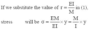
This expression of relationship between bending stress, the moment at the section and the sectional property is quite valuable. It is clear that the values of bending stresses will be at a maximum for the extreme fibres from the neutral axis. Suppose the farthermost fibre is at a distance of ‘a’ from the neutral axis. In this case,
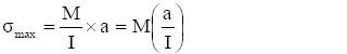
If the moment of inertia for a section is I, and the distance of the farthermost layer from the centroidal axis is a, the expression I/a is known as the section modulus of that cross section. It is expressed with the notation Z.

This is a refined form of the expression relationship among maximum bending stress, bending moment and the sectional properties. There can be situations when the overall sectional area is not symmetrical about the centroidal axis. Therefore, the distance of the outermost fibre on both sides of this axis will be different. In such cases, there will be two different values for section modulus, which will be used to work out the maximum bending stress on either side of the neutral axis.
It would be important to mention here that while deriving the stress formula for bending, it has been assumed that the section is subjected to only bending moments. As we are well aware, the forces that cause bending would also cause the shear force in the beam. Therefore, nearly the entire section would be subjected to combined bending and shear force. These shear forces would introduce warping in the sections and the section would no longer remain plain after bending. This goes against one of our basic assumption that after bending, the plain sections remain in the plain state only. However, further detailed analysis has proven that the presence of shearing stresses does not affect the development of the bending stresses and the values derived from the bending stress formula can be used safely for design.
3.4.1 Values of the moment of inertia for common sections
While discussing the bending stresses and deriving their expressions, we have seen the importance of the value of the moment of inertia for the section of the member. As defined previously, the moment of inertia for a section is the sum of the multiplication of all the elements of the area with the square of its distance from the centroidal axis of the area. Since the moment of inertia is the product of multiplication of the area with the square of the distance, its unit is the (length).4
It is always possible to derive the value of the moment of inertia for a section from the first principle, by applying the process of mathematical integration. However, while designing a section for a beam or any other member, we normally adopt the regular geometrical sections symmetrically distributed about one or more of its axes. Hence, it may be useful here to provide the expressions for the moments of inertia for some common plane shapes.
| Shape | Moment of Inertia (I) | Section Modulus (Z) |
|---|---|---|
| Rectangle – Breadth = b Height = h |
 – About axis X-X – About axis X-X – About axis Y-Y – About axis Y-Y |
  |
| Circle – Diameter = d |
 – About axis X-X & Y-Y both – About axis X-X & Y-Y both |
 |
| Triangle – Base = b Height = h |
 – About axis X-X – About axis X-X |
Parallel axis theorem
This theorem is very useful to work out the moment of inertia of an area with respect to any axis, as long as the value of the moment of inertia about an axis parallel to it is known.
As per this theorem, if the moment of inertia with respect to axis X-X is Ix, the total area of the shape is A and the distance of the new axis from X-X is d, the moment of inertia about the new axis is
Inew = Ix + Ad2
Illustration 3.1: We will determine the moment of inertia of the section shown in Figure 3.6, about the X axis passing through the top of the section.

Moment of inertial of a section – illustration 3.1
As is obvious, the section shown consists of two rectangles. The axis A-A’ is the one about which we have to determine the moment of inertia.
The moment of inertia of the top rectangle about its centroidal axis is
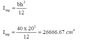
Similarly, the moment of inertia of the bottom rectangle about its centroidal axis is
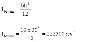
The area of the top rectangle is
Atop = 40 x 20 = 800 cm2
And the distance of its centroidal axis from A-A is
dt = 10 cm
As per parallel axis theorem, the moment of inertia of this segment about A-A is
| I’top | = | Itop + Atop dt2 |
| I’top | = | 26666.67 + 800*102 |
| I’top | = | 106666.67cm4 |
The area of the bottom rectangle is
Abottom = 30 x 10 = 300 cm2
And the distance of its centroidal axis from A-A’ is
db = 15+20 = 35 cm
As per parallel axis theorem, the moment of inertia of this segment about A-A’ is
| I’bottom | = | Ibottom + Abottom db2 |
| I’bottom | = | 22500 + 300*352 |
| I’bottom | = | 390000cm4 |
Therefore, the gross moment of inertia about A-A’ is
| I’ | = | I’top + I’bottom |
| I’ | = | 106666.67 + 390000 |
| I’ | = | 496666.67 cm4 |
3.4.2 The application of the principles of bending stress
We have seen in the expression for bending stress that the value of stress increases when the distance of the fibre from the neutral axis increases. In other words, the fibres located near the neutral axis would be less stressed in comparison to the fibres located at the edge of the section.
The other observation is that for a fixed maximum stress value, the moment-resisting capacity of a section is directly proportional to its section modulus, which is a function of the moment of inertia and overall depth of the beam. Therefore, it would prove economical if the moment of inertia of the section could be increased without altering the overall area substantially.
To see the achievement of these objectives, let’s start with the case of a beam with a rectangular section of b×h. The same is shown in Figure 3.7 (a).
As the stress generation is only due to the bending moment, the area adjacent to the neutral axis (which passes through the center of the area) is subjected to less severe stresses compared to the fibres at the extremity. As the material is assumed to be homogeneous, the stress on fibres at the extremity would govern the design, and fibres near the neutral axis would remain under-stressed. This is an example of inefficient use of the material in the construction.
It is obvious from the expression of the section modulus (for a rectangular section) that the value (of the section modulus) will be higher for a section with a higher depth-to-width ratio than for a section with a lower depth-to-width ratio, even if the area is the same in both cases. Therefore, the deeper section is more economical in comparison to a wider section of the same area. However, there is a limit beyond which the section will become laterally unstable and would tend to buckle.
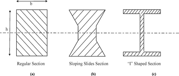
Cross section to withstand bending efficiently
We will try to develop a more efficient section now. Since the moment of inertia will increase if the area distribution is such that more of it is distributed away from the neutral axis, it may be helpful to provide the sides a slope away from the neutral axis. This arrangement is shown in Figure 3.7 (b).
With this, the value of the section modulus has increased and the section has become more efficient. However, it may not be convenient to form sloping sides during construction or fabrication. Therefore, another improvement can be taken up here. It may be decided to form wide flanges at equal distance on both sides of the neutral axis. As we can see from the parallel axis theorem, the value of the moment of inertia of this new arrangement about axis X-X would be substantially higher. Since two flanges alone cannot remain stable, a web has been provided to connect both with each other. This arrangement is shown in Figure 3.7 (c). The web also resists most of the vertical shear, as we will see later on.
This development of ‘I’- or ‘H’-shaped sections is one of the examples where the understanding of the development of bending stresses helps in more efficient use of the material in design.
Everything described above is true for a material that has similar strength in both tension and compression. However, there are materials that have lower tensile strength in comparison to compressive strength. Cast iron is one example of such materials. Now, if such a material is exclusively used for the construction of a beam, a section symmetrical about its X-X axis would prove uneconomical. This is because the tensile stress in the outermost fibre would reach its limit even when the stress on the compression face fibre has still not reached its limit. In this case, it would be more economical to design an asymmetrical section. Such a section would have its centroid nearer to the tensile face of the section. In such case, Zc would be less than Zt in magnitude. Since the magnitude of stress generated is inversely proportional to the value of Z, the value of tensile stress in the outermost fibre would always be less than the value of the compressive stress for the corresponding fibre. A ‘T’-shaped section is a classic example of sections useful under such situations.
We will now illustrate the process of bending stress determination with the help of an example.
Illustration 3.2: Figure 3.8 shows a simply supported beam of ‘I’-shaped cross section. The loading on the beam and the cross-sectional dimensions are described in the sketch. The objective is to find out the value of the maximum stress developed in the material at any section.
First of all, we will determine the maximum value of the bending moment, which is being generated due to this loading.

Bending moment diagram for an ‘I’ beam
As the load system is only vertical, the reaction at A and B will only be vertical.
Taking the moment about B and equating the same to zero:
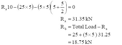
It is clear from the loading pattern that the maximum value of the bending moment would be generated at C, right under the concentrated load of 25 kN:
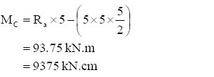
The resultant bending moment distribution is shown in Figure 3.8. The curved shape between A and C is the effect of the uniformly distributed load.
The next step is the determination of the moment of inertia of the beam section, with respect to the axis of bending. As we have seen, the neutral axis for a section passes through the centroid of the area. The ‘I’ section under consideration is symmetrical about both X and Y axes, respectively. Hence, the neutral axis would coincide with this axis of symmetry. The axis X-X is shown in the figure.
To calculate the moment of inertia about axis X-X, the three elements of the section have to be considered separately. These elements are:
- A vertical web of size 560 mm × 10 mm
- Two horizontal flanges of size 400 mm × 20 mm each
Both are rectangular sections and we know that the moment of inertia for a rectangular section about axis 
For the sake of convenience in calculations, we will adopt the cm unit of measurement of length.
Hence, Iweb = 1 × 563/12 = 14634 cm4
And, Iflange = 40 × 23/12 = 26.67 cm4 (for each flange)
It may be noted that the value derived for the moment of inertia of the flange is about the X-X axis of the flange itself and not of the overall section. For this conversion, we will be required to apply the theorem of parallel axis.
As per the theorem of parallel axis,
| Inew | = Ix + A×d2 | |
| Hence, | I’flange | = Iflange + Aflange × d2 |
| I’flange | = 26.67 + 40× 2× 292 | |
| I’flange | = 67306.5 cm4 |
It may be worth noticing here the amount by which the effective moment of inertia has increased per flange is due to a more efficient distribution of material with respect to the axis.
Therefore,
| Gross value of I | = Iweb + (2 ×I’flange) = 14634 + 2×67306.5 |
| = 149247 cm4 |
We also know that section modulus  , where y is the distance of the outermost fibre from the neutral axis. In this case, this distance is 30 cm.
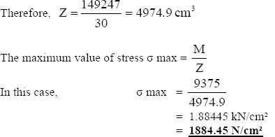
Therefore, the maximum value of the stress encountered by a fibre of the material would be 1884.45 N/cm2.
3.5 Shear force and bending moment – the relationship
We have seen in the previous section that a shearing force almost always accompanies the bending moment on a particular section on the section. The exceptions are very few. Even if a loading condition indicates a no-shear-force zone for a considerable length of span, such a state is unlikely in practice. This is because generally some of the loads will be non-stationary and would challenge this state of stable bending moment and shear force distribution. Therefore, the previously analyzed situation where the section is subjected to pure bending has little likelihood of being met.

Shear force and bending moment relationship
It would be interesting to observe the relationship of bending moment and shear force, when they are acting together at a section of a laterally loaded beam.
As shown in Figure 3.9 (i), a very small element of beam of length dx has been cut at two sections ab and cd respectively. These sections are subjected to both bending moment and shear force together. The magnitudes of bending moment and shear force however are different at both the sections.
Suppose the bending moment and shear force at ab are M and V respectively. Also, no force has been acting within the length dx; hence, the value of the shear force at both the sections will be the same. Let us say that the values of the bending moment and shear force for section cd are (M + dM) and V, respectively. As the element is in the state of equilibrium, the resultant moment about point c should be equal to zero:
M – (M + dM) + Vdx = 0
Vdx – dM = 0
Hence,  = V
= V
dx
The expression, , is the rate of change of the bending moment with respect to axis X. It means that the rate of change of the bending moment at a section is equivalent to the shear force.
While deriving this relationship, we have considered the situation where there was no external lateral force acting on the element abcd and value of shear force on section ab is equal to the corresponding value on section cd. However, there may be situations when lateral forces are acting on the element abcd in such a way that the values of shear force are different on faces ab and cd. These are shown in Figures 3.9 (ii) and 3.9 (iii). In Figure 3.9 (ii), a uniformly distributed load of intensity w per unit length is acting on the element. We can assume that the result has been working at the center of dx, or at a distance  away from the point c. In this situation, the values of bending moment and shear force at ab and cd are M and V and (M + dM) and (V + dV), respectively. In this state, equating the moment about c to zero,
M – (M + dM) + Vdx + wdx = 0
Since dx is a small quantity, its square would be an even more insignificant quantity and hence the value of wdx (dx/2) in the expression can be ignored. With this, the expression becomes

This relationship is the same as derived in the earlier case. Now, we will consider the equilibrium of the specimen under the influence of all the vertical forces:
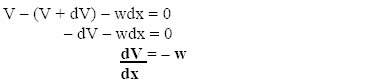
This relationship means that if a uniformly distributed load is acting on a beam, the rate of change of shear stress will be equal to the intensity of the negative of the uniformly distributed load. This is easy to understand as we have already seen in the analysis of beams.
Now consider the case of Figure 3.9 (iii), where a concentrated load of value W is acting on the element. As is obvious, the difference in the shear force on faces ab and cd would be equal to load W. Since the change in the shear force in this case is sudden, the value of dM/dx would become discontinuous at the section of application of the load.
3.6 Bending shear stress
In Section 3.4, we studied the influence of bending or flexure on a beam section. The bending moment, when converted into direct stress on the cross section, will have the distribution shown in Figure 3.10. In other words, if the beam section is assumed to be made from a number of thin layers of the material, each layer would have a different magnitude of force acting on it.
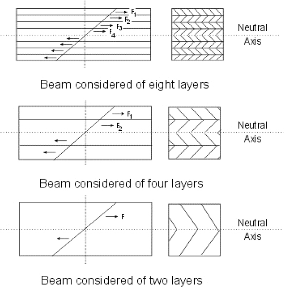
Beam layers
Just to make the explanation easy, we imagine the beam section to be formed of eight layers, as shown in Figure 3.10. The width of each layer is equal to the width of the cross section of the beam and the depth of each layer is h/8, where h is the overall depth of the section. Four of these layers are above the neutral axis of the section and the other four are below it.
To make it simpler, it is assumed that no vertical shear force is acting on the section and the value of bending moment is positive and similar on either side of the section. We know that the positive bending moment induces compressive stresses in the fibres above the neutral axis and tensile stresses in the fibres below the neutral axis.
We would see all the eight strips separate from each other with the corresponding force paragon. As we already know, the distribution of stress is such that the outermost fibres, i.e. the top and the bottom ones, would be under the most severe stress. Hence, the average stress for strip 1 will be higher than the average stress for strip 2. The average stress multiplied by the cross-sectional area of the strip would provide the magnitude of the force on the strip. Since the cross-sectional area of each strip is the same, the force on 1 will be more than the force on 2. When the section acts as a monolith, this difference between the force in strips 1 and 2 needs a balancing shear force along the interface of the strips, the magnitude of which is equal to the difference between the forces in strips above and below it.
Now, instead of each zone formed of four strips of depth h/8, we assume two strips of depth h/4 each. In this case, the difference of the force on the interface would be much larger compared to the earlier case. Therefore, the magnitude of the shear force to balance it would be much larger on this surface. It is clear that the magnitude of the shear force would be the largest if we consider a neutral axis as the interface.
It is now clear that the largest magnitude of the unbalanced shear stress exists at the neutral axis and the same decreases continuously towards the external layers on both the top and bottom of a given section. The shear force becomes zero at the outermost layers of the section.
3.7 Horizontal and vertical shear – relationship
We have seen that the material of the beams would be subjected to two kinds of shear stresses.
- The vertical shear stress, acting on the cross section of the beam that would be due to the imbalance of the vertical forces acting on one side of the section.
- The horizontal shear stress, which is generated due to unequal longitudinal strain in the fibres of the beam resultant to bending.
We will now try to see if there is some relationship between these two types of shear stresses.
For this, we consider the element of a beam, shown in Figure 3.11. The section of the beam is subjected to a vertical shear force of magnitude V. To balance this, a resisting shear stress of value τv has been developed on the vertical face.
Let’s examine the types of forces acting on the prismatic element ab of unit length of the beam, the width of which is m and the depth is n. We assume that for such small depth n, the distribution of the shear stress is uniform across the length of the element. Hence the shear stress of magnitude τv has been acting on the vertical face of the element and the shear stress of magnitude τh has been acting on the horizontal face of it.

Section of a beam
The free-body diagram of the element is drawn in Figure 3.12. For the equilibrium of the body, the bottom face of the element would be subjected to the force of the same magnitude, which is acting on the top surface of the element. The direction of this force will be opposite to the one on the top. Since the surface area on top and bottom is the same, both the faces will be subjected to the same shear stress τh.

Complementary shear stress
By the same logic, the stress development on both the vertical faces of the element will be of the same magnitude τv, though the direction will be opposite to each other. As emerges from Figure 3.12, the sets of horizontal and vertical forces will form two separate couples. The horizontal forces would form an anti-clockwise couple. To balance, the value of the couple formed by the vertical force set will be the same but the direction will be clockwise.
Equating both the couples,
| τh(n×m) = τv(m×n) | (the length of the element is unity) |
Hence, τh = τv
Therefore, there is a relationship between the horizontal and vertical shear stresses. The shear stress acting on a section of the member does induce a counter-balancing shear stress of the same magnitude in the plane parallel to the section.
3.8 Bending shear stress – determination
As established, there is a relationship between the vertical shear stress distribution due to the transverse loads and the horizontal shear stress distribution due to bending of the section. We have observed that the bending moment at a section of the member is represented by the distribution of the stresses across the section. The nature of these stresses and the pattern of their distribution also have been studied. Now we will see the pattern of the distribution of the shear stress due to a shear force acting on the section.
We again refer to Figure 3.11. The case of a strip of very small depth has been considered and it has been assumed that the horizontal shear stress for this is uniform. At the same time, we are aware of the following.
- Across the section, the value of the horizontal shear stress increases from the outermost fibre to the neutral axis, and attains its largest value at the neutral axis.
- There will be the presence of a shear stress of equal magnitude on the section perpendicular to the section of its direct application.
With these two facts taken together, we can guess the distribution pattern of the shear stress along the section, resultant from the application of the shear force of the magnitude V. The distribution of the stress would be such that the maximum value of shear stress is at the neutral axis, gradually decreasing towards the outer fibres.

Distribution of flexural stress
To observe the distribution of shear stress, we consider one element of the beam. As shown in Figure 3.13, a portion of the beam between sections aa’ and bb’, spaced dx apart from each other, is taken. The width of the section is b. The moment acting at section aa’ is M and at section bb’ is (M + dM). This is a common case in beams when the magnitude of the moments varies from section to section. The position of the neutral axis and the stress distribution on both the sections are shown in the figure.
Now to determine the actual value of the shear stress, we study the condition of equilibrium for a block between the two sections. The block we have selected is below the neutral axis and its top face cc’ is parallel to the neutral plane, at a distance y1 from it. The bottom face of the block is along the bottom surface of the beam.
To study the condition of equilibrium, the block ca’c’b’ is separated from the beam body and is shown as the free body with all the forces acting on it. Due to bending, the faces ca’ and c’b’ will be subjected to trapezoidal stress blocks, acting in a direction opposite to each other. Since the bending moments on the two sections are different, the trapezoidal stress blocks also will be dissimilar from each other. Hence, there would be a difference in the magnitude of the forces acting on both these faces. To balance, a shear stress of intensity τ will act on the top surface of the block. There would be no such shear stress on the bottom surface as it coincides with the bottom of the beam and, therefore, will be free from shear stress.
The force acting on an area dA on face ca’ of the block is

The entire force on face ca’ can be determined by integration of this expression within limits y1 and c (c being the distance of the bottom face of the block from neutral surface). Hence total force on the face ca’ is
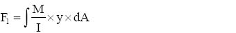
In a similar way, the magnitude of the force acting on the other vertical face c’b’ of the block is
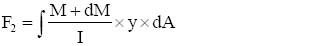
It is obvious that the balancing shear force acting on the top horizontal surface of the block will be equal to the difference of these two forces. As the value of the stress at this surface has been assumed as τ, the total value of the force on the face is
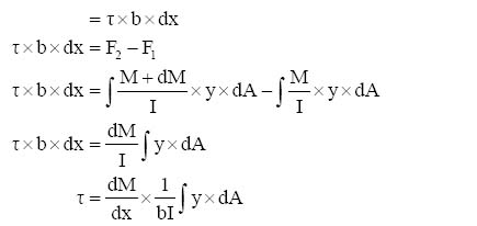
It can be recollected that in Section 3.5 on the relationship between the bending moment and shear force, we saw that the value of the expression dM/dx is equivalent to the shear force. Placing this value of dM/dx in the above expression,
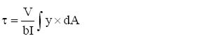
The expression ∫ y dA in effect means the sum of the moments of the area of the section about the neutral axis of the section. Since the range of integration has been y1 to c, it can be represented as the multiplication of the area of the block between depths y1 to c from the neutral axis, multiplied by the distance of the centroid of the block from the neutral axis. This expression is termed as the static moment of the area:
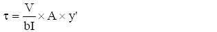
The static moment of area is expressed with the symbol Q.
| Hence, | τ = | VQ |
| bI |
This expression gives the value of the shear stress along the depth of the section. This can be utilized to observe the variation of stress along the depth of the section. It may be clearly noted here that while deriving the expression, the variation of shear stress across the width of the section has been considered as uniform. This assumption holds reasonably for most cases but is not true entirely. In the case of sections where flexural (or bending) stresses are not evenly distributed over a horizontal layer, the assumption would not hold good.

Shear stress distribution for various sections
Due to this reason, the value of shear stress derived for a rectangular section is normally accurate as the distribution of flexural stress is uniform. But if we take the example of the trapezoidal section, as shown in Figure 3.14(a), the value of shearing stress at the neutral axis of it will be at the minimum at the longer edge and at the maximum at the shorter edge. In such cases, what we would determine with the help of the shear stress formula would be the average value of the stress at the layer.
Let us consider another situation. In Figure 3.14 (b), shear stress distribution across a wide flanged section has been shown. The section is symmetrical about the X axis and therefore the distance of the neutral axis from the top and bottom layers is similar. Hence, the maximum value of the shear stress is at the center, and decreases toward the top and bottom edges (but not linearly). Suppose the value of the shear stress at the center is τmax and at the layers just on the inside of the flanges, i.e., at the surface mn, the value of the shear stress is τflange. The distribution of shear stress has been shown in the diagram.
Since in this case the shear stress at the inside free surfaces km and nl of the flange should be equal to zero, the distribution of the shear stress along mn and further within the flange would be quite complicated and definitely would not be uniform. This is another limitation of the formula for shear stress distribution determination, which needs to be kept in mind during its application for structural analysis.
3.8.1 Rectangular section – shear stress distribution
We have already derived the expression for the distribution of shear stress for any section. We will now see the distribution of shear stress along a rectangular section of height h and width b, as shown in Figure 3.15. The distance of the outermost fibres from the neutral axis is h/2, for both top and bottom.

Distribution of shear stress in rectangular section
We know that the value of shear stress at any layer is
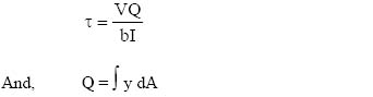
Now for a rectangular section, the area of the strip (dA) will be represented by b×dy. The upper limit of integration will also be h/2 in this case:
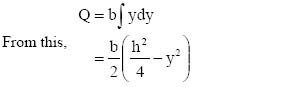
Substituting this value of Q into the expression,
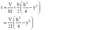
In this expression, V, I and H are constants for the particular section. Hence the distribution of shear stress across the section is parabolic (where the value of y is variable).
To determine the values at the center and at the edges, we will put the respective values of y in the expression.
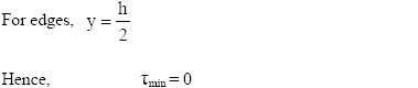
Therefore, the value of shear stress at the edges is zero. We have studied the reason for this.
For the center, y = 0
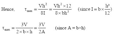
Here, V/A is the value of the average shear stress on the section. It means that the maximum value of the shear stress in a rectangular section is 1.5 times the value of the average shear stress on the section.
Illustration 3.3: We will see the application of shear stress distribution in the illustration below.
The beam AB, shown in Figure 3.16, is a simply supported structure of 8 m span with load W-N acting at the center of the supports. The width of the section is 15 cm and depth is 40 cm. The permissible stresses in the materials are as follows:
| In bending (tension as well as compression) = | 900 N/cm2 |
| In shear | = 100 N/cm2 |
The objective is to determine the maximum value of W, which meets the criteria of maximum stresses.

Section of a beam
For this case,
support reactions 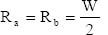
The maximum value of the bending moment in this case will be at the center of the span, as the concentrated load W has been acting on this section.
The bending moment at the center is  = 2 W N-m = 200 W N-cm.
The maximum value of the shear force will be at any of the supports and would be equal to W/2.
Hence, V = W/2 Newton.
The dimensions of the rectangular cross section are also known. The area and section modulus can be worked out on its basis.
Area is A = b×h = 15×40 = 600 cm2.
Section modulus is 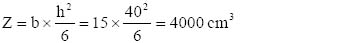 .
.
We know from the bending stress formula that
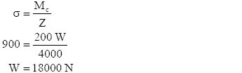
and from shear stress for a rectangular section that
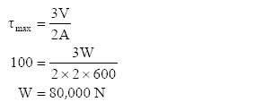
The permissible value of the load derived from the criteria of bending stresses is much smaller compared to a similar value derived from the criteria of shear stress. Therefore, it is clear that maximum bending stress will govern the design in the case and the maximum permissible value of W will be 18,000 N.
3.9 Deformation of beams
On many occasions, the resistance to deformation determines the design of a beam, a property termed as rigidity. Even when the beam section has an inherent strength to withstand high loads, the value of loads should be kept low to ensure that the degree of deformation is within acceptable limits. Alternatively, a section with higher sectional properties (area or moment of inertia) would be adopted even when a lower section’s properties meet the criteria of required strength. This is to ensure that the magnitude of deformation is within limit.
Deflection is one of the most critical measurements of deformation. Due to the application of loads on a beam and the resultant moment generation at the section, the beam adopts a new profile that is known as the deflected shape of the beam. We are limiting ourselves to the case of elastic deformation only. The other assumption here is that stress is proportional to strain, i.e., the material follows Hooke’s law.
3.9.1 Elastic curve
The projection of the neutral surface of the beam in a vertical plane, when the beam is in the state of deflection, is known as the elastic curve of the beam. If the equation of the elastic curve is determined by some method, it would give the relationship between the x and y coordinates of the beam and can be used to determine the value of deflection (y) at any section of the span (x).
To determine such an equation, we refer to Figure 3.17. The elastic curve OB of a prismatic beam has been shown. We consider a small element pq of the elastic curve. The length of ‘pq’ is ds and its projection on the X axis is dx. The tangents drawn at points p and q form an angle of value dθ between them.
The curve pq has its center at C and the radius of curvature is r. We know from geometry that the normals drawn from C to the points p and q also form an angle dθ between them. The deflections in this case are assumed to be very small compared to the overall dimensions of the beams. This is actually true for almost all real-life situations. Due to this, the difference between the length of the deflected shape of pq and its projection on X axis is very small. Therefore, ds = dx.
The value of the slope between any two points of the curve is
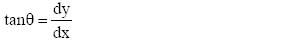
Again since the deformations are very small, θ would be a very small value. In such a case,


Elastic curve
Differentiating the expression further with respect to x,
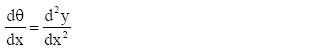
Also, if we consider Cpq as a triangle with its arm ‘pq’ equal to dx,
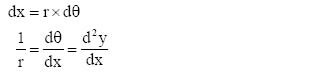
In Section 3.4, we have seen the establishment of a relationship for r. As per Section 3.4,
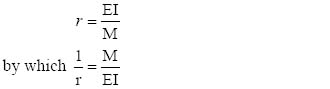
This, along with the previous expression for 1/r, establishes the relationship
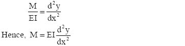
This expression is the differential equation of the elastic curve for the beam, which is subjected to bending. When it is solved to bring to the form y = f (x), it would give the true equation of the elastic curve. For this, we would twice integrate the equation with respect to x. On first integration,
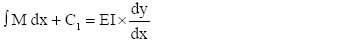
where C1 is the constant of integration, the value of which is required to be obtained for a given condition of loading.
In the above expression,  is the value of the slope of the elastic curve at that point. It is the angle which the tangent drawn at the point forms with the original axis of the beam. Since the beam generally has a horizontal axis, the slope at any point will become the angle between the tangent drawn at the point and the X axis.
On second integration,

This is the desired equation for the elastic curve. The value of the second constant of integration C2 also needs to be determined for the given loading condition.
This method of determination (of the equation of an elastic curve) is known as the method of double integration. As stated, values of constants C1 and C2 are dependent on a given loading condition. It implies that the equation of the beam has to be written all over again whenever the loading condition changes. This limitation can be overcome by writing the equation in such a form that its applicability remains for the entire span. Carefully selecting and ignoring the applicable portions of the equation further achieves this.
Illustration 3.4: We will take up the following example to determine the equation of the elastic curve and the maximum deflection for a simply supported beam, if the beam is loaded with a uniformly distributed load of w intensity per unit length, throughout the span.
As shown in Figure 3.18, the beam OB is a simply supported one with span L. The loading intensity, as described above, is w per unit length. The beam is prismatic so the value of the moment of inertia is constant throughout the span.
We know that
Ro = Rb = 
To determine the equation of the elastic curve, we assume that point O at one end of the beam is the intersection of X and Y axes. Consider a point A along the curved shape of the beam, the abscissa of which is x:
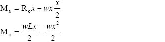
Replacing M with the value derived in Section 3.91,
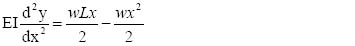
Integrating both sides with respect to x,
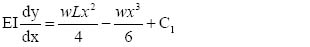
Here, C1 is the constant of integration. To find out its value, we will first have to find a defined situation for the slope, since represents the slope of the elastic curve. In this case, since the loading is symmetrical about the center of the span, the value of the deflection will be the largest at the center of the span. Therefore, the tangent at this point of the elastic curve will be parallel to the X axis, with its slope with respect to the X axis being zero. Mathematically,
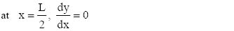
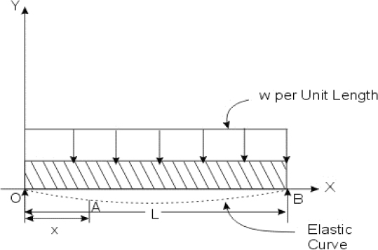
An elastic curve
Substituting these values in the expression above,
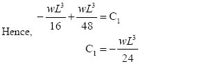
Putting this value of C1 back into the equation,
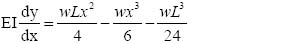
Taking the integral of both sides once again,
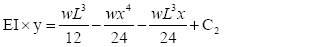
To find the value of C2 of this expression, we would look for a defined value of deflection y, which would be consistent with the arrangement. In the case, since both the ends of the beam are supported, the value of deflection at any of the support is nil.
Mathematically,
for x = 0, y = 0
Substituting these values into the above equation yields that the value of C2 is zero.
Just from the academic point of view, if we put the values x = L and y = 0 in the expression, which is the case for the end B, the result obtained would be similar.
Hence, the equation of the elastic curve is
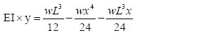
After deriving the equation for the elastic curve, the next objective is to find the value of the maximum deflection. As explained earlier, the value of the deflection will be the maximum for the center of the span, i.e., at x =  .
.
With this,
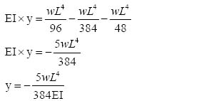
The negative sign indicates the direction of the deflection with respect to the X axis.
3.9.2 Moment area method
Moment area method is another popular method of determining the values of deflection and slope for a structural element, which is subjected to bending. The principle of the method is the same as for the earlier explained method of double integration.
Again refer to Figure 3.19. LN is the elastic curve under consideration. The bending moment diagram for the same due to loading is L’N’. The tangents drawn at L and N are LL1 and NN1 respectively. The angle between the two tangents is θ. A very small portion of the elastic curve of length ds subtends an angle dθ center C of the arc.
As we have seen in Section 3.9.1, for similar elastic deformed body, which follows Hooke’s law,
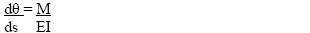

Elastic curve – moment area method
Since ds is very small and its curvature is not very steep, we replace ds with dx – the projection of the arc on the X axis:
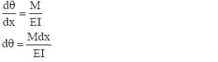
Graphically, the value of Mdx is equal to the area of the bending moment diagram for portion ds. Since dx is a very small length, the value of the bending moment along this length can be assumed to be uniform, although it might be varying from section to section.
Now, to determine the value of the angle θ, both sides of the expression will be integrated between the limits L and N:
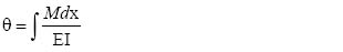
The expression on the right-hand side is the total area of the bending moment diagram for the entire span LN of the beam, divided by EI.
In the same Figure 3.19, dt is the intercept which the tangents drawn on both the ends of the curve element ds, cuts on an axis along N that is perpendicular to the original axis of the beam. Since the distance of the segment from point N is x and the angle between two tangents is dθ, the intercept dt may be considered equal to the arc of the circle with radius x subtending angle dθ at the center. From this relationship,
dt = x dθ
Putting the value of dθ from the earlier derived expression,
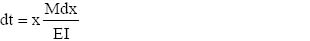
We can see that the distance measured perpendicular to the original axis of the beam from N that will intersect a tangent drawn from end L of the elastic curve will be equal to the sum of such intercepts for all segments of the curves between the two extreme points. From the above expression this can be derived by integrating both sides of the expression within limits L and N:
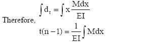
The expression ∫x Mdx is the ‘moment of the bending moment diagram’ with respect to N. It may be noted here that the length of the intersection is required to be measured from the point where the perpendicular cuts the elastic curve. Since we have considered the case pertaining to the extreme points of the elastic curve (which do not yield during deformation), the original distance remains unchanged after the deformation.
Another aspect that needs attention is that the expression (above) provides the value of intersection at the line through N perpendicular to the original beam axis. Consider the case when we need to work out the corresponding value of intersection at the line through L when the tangent has been drawn at N. In this situation, the value of ∫ x Mdx is the moment of bending moment diagram with respect to L. Although the bending moment diagram is similar in both the cases, the length of the moment arm (x) will be different except for the case when bending moment diagram is symmetrical about both the points. In normal situations,
t (n-l) =/= t (l-n)
3.9.3 Moment area theorems
On the basis of what has been derived in this section, we define the two moment area theorems as below.
Theorem – I : For an elastic curve, the angle between tangents at any two points on the curve is equivalent to the total area of the bending moment diagram between these two points, divided by EI.
Theorem – II : For an elastic curve, the deviation of any point perpendicular to the original beam axis, relative to the tangent drawn on the curve at any other point, is equivalent to the moment of the area of the bending moment about the first point, divided by EI.
In both the above theorems, it is assumed that EI, the product of the Young’s modulus for the material and the moment of inertia of the section, is a constant. This product EI is known as the flexural rigidity of the section. For it to be a constant, both E and I are required to be constants. For it to be true, the material of the beam should be homogeneous so the value of E remains unchanged throughout. Also, the section of the beam is uniform (please remember, we have assumed the member to be prismatic), so the sectional properties remain unchanged.
These conditions are to be kept in mind while applying the theorems. In the case that the value of either E or I or both are not constant throughout the span of the beam, the pattern of their variation with respect to x will be needed for the application of the theorem. To simplify such situations, the ordinates of the bending moment diagrams itself are drawn to directly give the value of M/EI instead of just M, and the same M/EI diagram is used for the application.
3.9.4 Moment area theorems – applications
With the application of the moment area theorems, it is possible to determine the values of the slope of an elastic curve or the deflection of a point on it, in a semi-graphical way.
To obtain the desired values of the slope at any point, note the following procedure. As a first step, draw the bending moment diagram due to the load systems on the beam. We have learnt the procedure of drawing a bending moment diagram and therefore it should not be difficult.
However, we eventually would be required to accurately work out the area of the bending moment diagram and, in view of this, we may be required to follow a number of additional steps.
For this purpose, it becomes necessary in the case of multiple loadings to draw separate bending moment diagrams for each type of load. We know that the bending moment diagram for a concentrated load does form a triangular shape. The calculation of the area of this triangular diagram and determination of the centroid of this area are not difficult. If the load is uniformly distributed or gradually varying in nature, the shape of the bending moment diagram will be a curve.
As stated earlier, to solve the problem of the determination of the area of bending moment diagrams, it will be helpful if we break it into a number of simple structural situations.
For a loaded cantilever beam, the general expressions for the area and the centroid of such shapes are as follows:
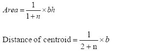
Here, b is the length of the base of the curve and h is the maximum ordinate or height of the geometric shape. The value of n would be dependent on the nature of the loading.

Moment diagrams under various loadings
The cases representing various types of loading on a cantilever beam and the corresponding bending moment diagrams are shown in Figure 3.20. The areas of such diagrams and their centroid locations have been tabulated below.
| Type of Load | Maximum Bending Moment (h) | Area of the Bending Moment Diagram | Distance of Centroid from Fixed End |
|---|---|---|---|
| Concentrated (W) | W.L | (1/2)b.h | (1/3)b |
| Uniformly Distributed (w per unit) | wL2/2 | (1/3)b.h | (1/4)b |
| Uniformly Varying (zero at one end to w per unit at the other) | wL2/6 | (1/4)b.h | (1/5)b |
While determining the area of the bending moment diagram and the distance of its centroid, the effort lies in reconfiguring the loading on the beam such that each part of it is similar to one or the other standard loading condition.
The illustration of the procedure to determine the area and centroid by solving the case ‘by parts’ has been given below.
Illustration 3.4: We have taken the case of the simply supported beam AB of 4 m span, with a concentrated load of 5000 N acting at the center of the span and a uniformly distributed load of intensity 400 N/m acting on the right hand half of the beam. The arrangement is shown in Figure 3.21.
From statics,
Ra = 2700 N
Rb = 3100 N
As a first step towards the solution, assume that the end B has the capacity to withstand moment. For this purpose, we assume the end B is a fixed end. Now with B as fixed, we consider the effect moment generating effect of Ra alone, by removing the other loads from the system. Note that the removal of these loads will not change the value of Ra.

Movement and distribution
Hence, Mb1 = 2700 × 4 = 10800 N.m.
This moment is positive in nature and the distribution along the span is shown in Figure 3.20.
Similarly, considering the presence of the concentrated load alone at the mid span,
Mb2 = 5000 × 2 = 10000 N.m
This is a negative movement and the distribution is shown again in Figure 3.20.
Finally, considering the presence of the uniformly distributed load alone at the right half of the span,
Mb3 = 400 × 2 × 2/2 = 800 N.m
The sign of this moment is also negative.
Before moving further, we observe that the value of the overall moment at B has been arrived as zero (10800 – 10000 – 800), which is consistent with the support condition at B. We have analytically and graphically shown the breakup of the moment generation due to load components.
If we plot these three moment diagrams on a common baseline, we obtain the actual bending moment diagram due to loading.
Now, we want to determine the area of the bending moment diagram due to the cumulative effect of loads. This area A will be equal to
A =A1 + A2 + A3
Here, A1, A2 and A3 are the areas of the respective bending moment diagrams due to individual loading. By substituting their values in the equation
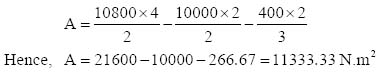
As per theorem 1 of the moment area, the angle between the tangents at A and B of the elastic curve will be equal to the area of the bending moment diagram between A and B, divided by EI.
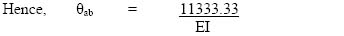
Again, the moment of the overall area about B can be determined by applying the principle of the parts:
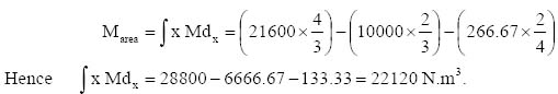
By applying theorem II of the moment area, the length of the intercept from B on a line drawn perpendicular to the original axis, by the tangent drawn from A,
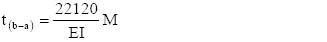
We have seen the procedure to determine the area of the bending moment diagram between two points on the span of the beam. We have also seen the procedure to determine the moment of the bending moment diagram about a point by determining the centroids of the part bending moment diagrams. When the results of this exercise are used in conjunction with the moment area theorems, we can derive the following deformations for an elastic curve:
- Slope between the tangents drawn at the two points
- Length of the vertical intercept from one point of the elastic curve by the tangent drawn at another point along the curve.
Although the second information is useful, our main objective is to find out the deflection of a particular point on the elastic curve from its original position. This information will not be directly available from the expressions we have seen so far, except for the condition when the beam under consideration is a cantilever. This is because, with a cantilever, due to a no-rotation condition of the fixed end, the tangent drawn on this point of the elastic curve coincides with the original axis of the beam. Therefore the intercept between the tangent and any point on the elastic curve would be equal to the deflection of that point with respect to its original position on the beam axis.
This point can be further understood with the help of Figure 3.22. Beam AB is a cantilever with load W acting at its free end B. Due to the action of the load, the beam will deform to the shape shown in the diagram.

A cantilever’s elastic curve
Consider point C in the original beam, which takes position C’ in the deformed beam. The tangent drawn at A clearly coincides with the original beam axis. Now we draw a line through C’, perpendicular to the original beam axis. The perpendicular distance between C’ and the original axis of the beam is the deflection at point C. At the same time, this distance is equal to the intercept between point C’ and the tangent drawn from A. As per the second moment area theorem, the value of this intercept {t (c-a)} will be equal to the moment of the bending moment diagram between A and C, with respect to C, divided by EI.
Illustration 3.5: We will consider the case of a cantilever beam AB of 4M span, with a single concentrated load of 2000 N working at the middle of the span at point C. We want to determine the deflection at the points:
- Right below the application of the load
- At the free end of the cantilever.

Determination of deflection
The structural arrangement and the bending moment diagram have been shown in Figure 3.23. The vertical reaction at B is equal to the total vertical load 2000 N.
As is clear, there has been no force acting in the portion CB of the beam and therefore there is no bending moment in the region between C and B. In the region AC, the bending moment distribution along the span has been shown in the bending moment diagram. The distribution is triangular with a maximum value of 4000 N.m at A and reduces to zero at C in a linear fashion.
Note the shape of the deflected beam or the elastic curve. The portion of the elastic curve between A and C’ has curvature of some degree. This curvature is the function of the shape and area of the bending moment diagram between the points lying in section AC’. At the same time, the shape of the elastic curve between C’ and B’ has been a straight line. The explanation for it from a physical point of view is that there has been no load acting at this section, which can intervene to alter the slope of the elastic curve; hence, the slope between C’ and B’ remains unchanged. Alternatively, as there has been no bending moment between C’ and B’, the slope between any two points taken between C’ and B’ would be zero (as per the first moment area theorem).
To determine the value of deflection at midpoint C, we will use the second moment area theorem. According to the theorem,
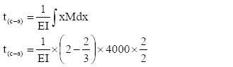
Note that the moment is being taken about point C of the bending moment diagram and hence the length of the moment arm is (2 – 2/3):
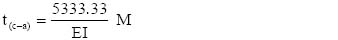
Similarly, to determine the deflection of the point B at the free end,
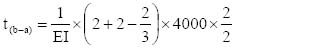
The area of the bending moment diagram  will remain unchanged in the case. What may be noticed is the change in the length of the moment arm:
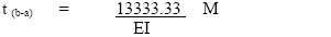
In this illustration, we have seen the method to derive the deflection at a point for a cantilever. When the beam under consideration is not a cantilever but a simply supported beam, we can still use the moment area theorem to derive the value of the deflection at a point of it. In this situation, however, there will be some additional steps required in the procedure.
To explain this, we take the simply supported beam AB of span L, as shown in Figure 3.24. The elastic curve of the beam has also been shown in the diagram. It is clear that the points at ends A and B are unyielding due to the support’s constraints and, therefore, they continue to remain at their original positions even after the deformation.

Determination of deflection
Consider a point C (in the original beam axis), whose deflection we want to determine. Point C is located at a distance l from point A. After the deformation, the point deflects by δ and assumes its new position at C’.
A tangent has been drawn at A, which cuts the line through B and perpendicular to the original axis at D. The intercept BD is t (b-a), the value of which can be determined from the second moment area theorem.
In the same way, the value of the intercept C’C’’, which is t (c-a), can also be determined. Once the values of t(b-a) and t(b-a) are known, we move forward by applying the principle of geometry. In Figure 3.24, the lines CC’’ and BD are parallel to each other. Therefore, ΔABD and ΔACC’’ are similar triangles.
From the properties of similar triangles,
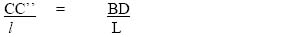
Here, CC’’ is the sum of the deflection of point C (δ) and intercept at C’ [t(c-a)]. Putting these values in the equation above,
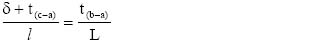
In the above expression, we know the values of all except δ. Hence, by putting all respective values in the expression, it is possible to determine the deflection δ for the point.
We will see the illustration of this method, too, with the help of the following example.
Illustration 3.6: Take the case of a simply supported beam XX’ of span 5 m. A concentrated load of 2000 N has been applied at point A, 3 m away from end X. We will see the determination of deflection at the point of application of load.

Structural Arrangement and the Bending Moment Diagram
Figure 3.25 illustrates the structural arrangement and the bending moment diagram. First of all, the reactions at both the supports X and X’,
Rx = 800 N
Rx’ = 1200 N
To draw the simplified bending moment diagram, we will assume end X’ as fixed one and consider one by one the moment generation effect of reaction Rx and vertical load.
Due to Rx, moment at X’ = 800 × 5 = 4000 N.m (+ve).
Due to 2000 N load, moment at X’= 2000 × 2 = 4000 N.m (–ve).
As shown in the representation of elastic curve in Figure 3.25, t (a-x) and t (x’-x) are the two intercepts of our interest. As per the second moment area theorem,
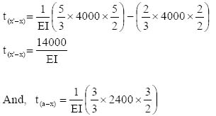
The triangular bending moment diagram between A and X would have a height equal to 2400 N.m at A. This results from the characteristics of the similar triangles.

From the elastic curve diagram of the beam,
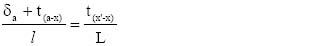
Here, δa is the deflection of point A with respect to its original position. Putting values in the expression,
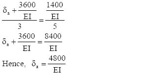
Therefore, the deflection at A would be equal to  .
.
The estimation of the deformation of a structure, or its element, is important from the functional point of view of the structure. On occasions, despite the stresses remaining within limit, the deflection of the structure may become excessive. Excessive deformation of a structure can lead to two problems.
- The finishing over the main structure members (for instance plastering over concrete beams and paint-coating over steel beams) may not be able to withstand large deformations and may loose its integrity.
- The second reason is psychological. Excessive deflection can affect the aesthetics of the structure and can also make users fear the safety of the structure.
To overcome this, structural engineering codes prescribe means to limit the deformation of structural members. As we can see from the expression of deflection for a particular structural arrangement and loading, the amount of deflection varies only with the variation in the modulus of elasticity (E) of the material and moment of inertia (I) of the section. In fact, the value of deflection is inversely proportional to the product of the two. Here, we may consider even the modulus of elasticity as non-variable as the material of construction is finalized beforehand, the selection being based on several factors. Hence the only variable remaining in the expression is the moment of inertia. We know that the value of I depends on the geometrical properties of the section and can be controlled by altering the sectional dimensions or the pattern of distribution of the material about the neutral axis.
To overcome the adverse effect on aesthetics, the practice has been to introduce the deformation of reverse order in the structure at the stage of construction. This is done by accurately assessing the value of future deformation under load and introducing the deformation of similar magnitude in the reverse direction at the time of construction or fabrication of the structure. This takes care to neutralize the deformation, which takes place when the intended loads are applied on the structure during its life.
3.10 The case of combined stresses
In the previous section, we studied the effect of direct loads and direct stresses (tensile and compressive) generated. We also studied the mechanism of stress generation at any section, due to bending moment and shear force. It is very clear how the value of stress can be determined if any one kind of load is acting on the structure.
But the application of a single kind of load may not always be the case a structural engineer encounters during analysis. There are occasions when the load application on a structure is such that it produces a combination of stresses. For instance, a beam subjected to loads normal to its axis may additionally be subjected to loads along its axis. In this case, the stresses induced at a section are a combination of direct and flexural stresses.
Take the example of beam AB, as shown in Figure 3.26. The beam has a span of L and a cross-sectional area of A. The beam is subjected to a load normal to its axis, which generates a bending moment at the beam’s cross sections. Apart from this, the beam is also subjected to an axial compressive load of magnitude W.
We will consider a section m-n along the span of the beam. Suppose the moment at this section is M.
Considering first the effect of flexure on the section m-n, the distribution of the stress along the section is as shown in Figure 3.26 (a). If the moment of inertia of the section about the axis of bending is I and the distance of the extreme fibre from the neutral axis, both on tension and compression face, is y, the extreme flexural stress at the section will be
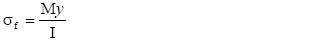

Combined bending and axial load
The value of σf would be unchanged for both tension and compression.
At the same section m-n, the distribution of the direct stress is shown in Figure 3.26 (b). The value of the direct compressive stress will be
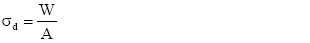
The magnitude of the combined stress at any layer of fibre will be equal to the algebraic sum of the stresses due to flexure and direct load at that layer. We want to work out the value of combined stress in the topmost and bottommost layers, as they would be the extreme values under the situation.
As is obvious, for the topmost layer, the direct compressive stress neutralizes the value of the tensile flexural stress to the extent of its own value (assuming that the value of flexural stress is larger). Hence, the net tensile stress on the top fibre is
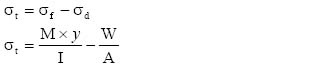
By the same logic, for the bottommost layer, the direct compressive stress adds to the value of the flexural compressive stress. The net compressive stress at the bottommost layer is
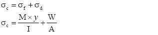
The distribution of the net stress across the section is shown in Figure 3.26 (c). It may be noted here that due to the combined effect of the stresses, the position of the neutral axis has shifted.
It is obvious from the above that if an optimum magnitude and type of direct stress is chosen, it is possible to control the net value of the stress at any fibre of the section. This concept has its application while designing with materials with unequal strength in tension and compression. As we will see in the section on reinforced concrete design, the same has been used to conceptualize and design the pre-stressed concrete members.
3.10.1 Combined stresses in columns
A column or strut is a structural member, which is predominantly subjected to axial compressive loads. Strut is a general term to define the members under compression, irrespective of the position of their axes with respect to the horizon. A column is a strut, which has its axis vertical.
We are quite aware of the effect of direct loads and also know the pattern of stress generation. We know that axial loads generate even stress along the cross section of the member. At the same time, this situation is valid under the assumption that the load is acting along the axis of the member. Any variation from this assumption would lead to a different stress development pattern across the section. We will observe the effect if the load application is off the axis.

Eccentric load on column
Let’s take the example of the column AA’. For simplicity, consider the cross section of the column to be rectangular with dimensions b × d. As shown in Figure 3.27, the column is subjected to a vertical compressive load of magnitude W. The application of load is at a distance e from the axis of the column. To analyze this situation, at A we introduce forces Wu and Wd acting vertically upward and downward respectively, along the axis of the beam. The magnitude of each force is equal to W. Since Wu and Wd do neutralize each other, the overall structural arrangement remains unaltered.
This combination of forces W, Wu and Wd can be considered to be acting in the following ways:
- The force Wu acts along the axis of the column.
- The forces W and Wd, being equal and opposite, form a couple with force W and arm e.
The couple induces a moment along the entire length of the column. The magnitude of the moment is
M = W×e
It is clear to us from the previous sub-section that due to the combined effect of the moment and direct force, the stresses on the outermost fibres of the column section would be
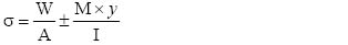
As  is the compressive stress, the use of the positive sign will give the value of the maximum compressive stress and the use of the negative sign will give the value of the maximum tensile stress on the section.
As is evident from Figure 3.26, the position of the neutral axis of the section is now not along the principal axis but is at a distance x from it. By definition, neutral axis is the location of zero stress. To find its location, we equate the value of the stress to zero:
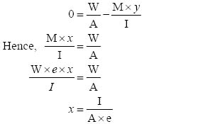
The above expression defines the shift in the location of the neutral axis if combined bending and direct forces are acting on it. It is a general expression for all the cases. In this case, when the section is rectangular with known dimensions,
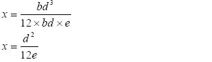
Therefore, for a given section and load, the shift in neutral axis due to eccentric application of direct load is inversely proportional to the amount of eccentricity.
It is obvious that the shifting of the neutral axis is accompanied by a reduction in tensile stress on one extreme of the cross section. The height of the triangular stress diagram will keep on decreasing as the neutral axis shifts towards the extreme edge of the section. It will become zero when the neutral axis coincides with the edge. This is the limiting condition when there is no tensile stress on any fibre of the section. In this situation, the shift in the neutral axis (x) is equivalent to one half of the overall depth of the section. Figure 3.28 can be referred to for clarity.
Putting this value of x in the expression above,
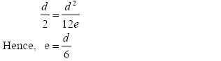

Neutral axis for eccentric loading
Therefore, in the case of a rectangular section, the value of extreme stress would remain compressive as long as the application of compressive load is within the inner one-third depth of the section.
3.11 Analysis of columns
In the previous sub-section, we studied the behavior of a column under eccentric loading. In general, columns are very slender members. This means that their lateral or sectional dimensions are quite small compared to their heights or lengths. The slenderness implies that the stiffness or rigidity of the section is low, which leads to excessive deformation. The photograph of a concrete column with its foundation is shown in Figure 3.29.
Columns can be described as short and long. A short or stub column is usually defined as one which has a length not more than ten times (or twelve times, as per some codes) its smallest lateral dimension. Hence, a column of section 20 cm × 40 cm is treated as a short column as long as its length is within 2 m. For any higher length, the same column would classify as a long column.
In an ideal situation, a column is assumed to be a member made of homogeneous material that is quite straight before the application of any load. Assuming the above statement true, the stress distribution on any section should remain uniform as long as the compressive load is acting along the axis. But in practice, nothing goes as assumed. The material is hardly homogeneous and there are some imperfections. The column, being a long member, would hardly be straight, even if this is undetectable to the naked eye. Some bending and crookedness would be unavoidable during the construction and erection of columns. On top of all of this, it is practically very difficult to avoid the eccentricity of loading. Worse, it is even more difficult to accurately assess each of these imperfections and apply corrections during analysis.

Concrete Column
Basically, it is clear that when we intend to have a straight long axially loaded column, we actually get a situation where the column is eccentrically loaded. This eccentric loading results in a moment and flexural stresses on the section, as we have seen previously. The moment causes the member to deform and due to the large length and low moment of inertia, the deformation is quite large and noticeable. This phenomenon of lateral deformation of columns under the action of direct loads is known as buckling.
In the case of long columns, the flexural stress or the buckling governs the failure and the importance of direct compressive stress is relatively low. Despite this knowledge, it is not possible to determine the rate of change of flexural stress with the change in the magnitude of the direct stress. Efforts have been made to address this uncertainty by deriving various formulae for different loading and end conditions for the columns.
3.11.1 Critical load – Euler’s column formula
Consider the case of a long column AB, the bottom end A of which is built-in and the top end B is free. The column is shown in Figure 3.30. We assume that the column has a perfectly vertical axis, homogeneous material properties and constant section throughout its length. The column has first had a horizontal force H applied at A, normal to its axis. Due to this, the end A deflects and assumes a new position A’, as shown in the diagram. At this stage, a compressive force P is applied along the axis of the column. Keeping P in position, the force H is removed. The free end of the column comes back to its original position at A.

Buckling of column
This exercise is repeated with a gradually increasing magnitude of vertical force P. The end A will continue to come back to its original position on the removal of H, until the force P reaches a certain magnitude. At that magnitude of vertical force, the end A of the column would continue to stay at its new position A’, despite the removal of the horizontal force H. At this stage, the column is treated as failed due to lateral buckling. The minimum load, on the application of which a column fails due to lateral buckling, is known as the critical load for the column. The notation for it is Pcr .
Euler, a Swiss mathematician, theoretically analyzed the failure mechanism of long columns and from there derived the expression for critical load. He based his analysis on the solution of the differential equation for the elastic curve of the column. Euler solved the expression for moment,  , for the condition of buckling. Based on his analysis, the expression for critical load is as follows:
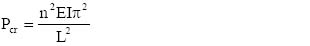

Degrees of column buckling
The above expression for Pcr is for the column of length L, both the ends of which are hinged. The value of n in the expression depends upon the shape of the column axis after the buckling.
The cases for values of n = 1, 2 and 3 are shown in Figure 3.31. Out of this, the shape representing n = 1 is the most common and is encountered frequently. For this situation, the value of critical load,
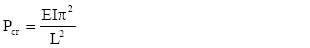
The buckling conditions for which n = 2, 3, etc., are not very common. These are possible if the column is provided with bracing. It may be noted here that for the same length of column, the bracing at midpoint would increase the value of critical load (and therefore the ultimate load carrying capacity of the column) to four times. Similarly, the bracing at one-third and two-third length of the column would increase the value of the critical load to nine times.
On analyzing the expression for critical load of a long column, we observe the following:
- The value of the critical load for a column depends on the length of the column (effective length, as we will see under the next observation) and the values of modulus of elasticity of the material and the moment of inertia of the section. It is independent of the strength, or the stress carrying capacity, of the material of construction. Therefore, the critical load for the columns made of different grades of steels will be the same, as long as the effective length and the sectional properties are similar. This is due to the fact that despite the large variation in the strength of the various grades of steels, the values of the moment of elasticity for them remain in a very close range.
- The length L in the equation is the effective length of the column arrangement. In the fundamental case, when both ends of the column are hinged, the effective length is equal to the overall length of the column. For any other end position, the effective length of the column would vary. In general, the effective length is considered as the length between the points of inflexion in the column. Let’s consider the situation where both ends of the column are fixed. If we draw the bending moment diagram, the points of inflexion fall at distance L/4 from both ends. Therefore, the distance between the points of inflexion is L/2, which has to be treated as the effective length of the column. Putting this value of effective length in the expression, we discover that the value of critical load has increased to four times compared to the case when both the column ends were hinged.
The different end conditions for column and their effect on the value of critical load are tabulated below.
| End Condition | Effective Length (L) | Factor for Critical Load with respect to Base Condition of Both Ends Hinged |
|---|---|---|
| Both Ends Hinged | L | 1 |
| One End Hinged and Other Fixed | 0.7 L | 2 |
| Both Ends Fixed | 0.5 L | 4 |
| One End Fixed (Built-in) and Other Free | 2L | 1/4 |
A column will always tend to buckle in the direction where the moment of inertia is the lowest. Due to this, it is necessary to put the value of the least moment of inertia of the column section in the expression while determining the critical load.
3.11.2 Use of Euler’s formula and its limitations
Euler’s formula provides the value of the critical load on a long column by the expression
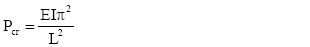
If we divide both sides by the area of the cross section of the column A:
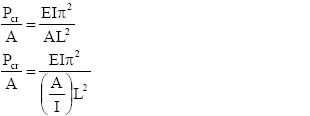
The value of expression√(I/A) is called the radius of gyration of the section and the notation for it is r. Also, Pcr/A is the stress on the section during critical load and is denoted as σcr. Putting σcr and r in the above relationship,
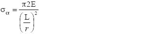
This ratio L/r is known as the slenderness ratio of the column. If for a given material, a graph is plotted between values of the critical compressive stress (σcr) and slenderness ratio (L/r), its shape would be as shown in Figure 3.32.
It is obvious to us that Euler’s equation to determine compressive stress is valid only if the value derived by it is less than the permissible compressive stress as per Hooke’s law. Since Euler’s formula does not recognized the concept of the proportionate limit of elasticity, the value of critical stress derived for shorter columns (of lower slenderness ratio) may exceed this stress limit. This is one of the limitations of the formula and is required to be kept in mind during application.

Slenderness ratio
By putting the value of the proportionate limit stress (σpr) in the expression above, we can find the value of slenderness ratio, for which σcr is equivalent to σpr.
The graph in Figure 3.32 can only be used when slenderness ratio values are above this limit. The portion of the graph, where σcr is more than the value of σpr, has been shown with broken lines and should be ignored during analysis.
The other important aspect is that the value of critical stress determined by Euler’s formula is the ultimate or failure stress. One can notice that at any stage, no factor of safety has been introduced in the expression. Therefore, it is important that once critical stress has been determined, it be suitably factored to derive permissible stress.
We will demonstrate the steps involved in the analysis of columns, with the help of an illustration below. In this illustration, instead of providing a specific solution to a design related problem, how one should proceed and use the various design inputs is shown. The reason for this is that to derive the permissible value of critical stress for a given slenderness ratio, we need the related stress graphs or tables for the material under consideration. It would not be convenient to reproduce them on these pages and once the concept is understood, applicable codes can be referred for them.
Illustration 3.7: Take the case of a rectangular section of the size 4 cm X 6 cm. It has been made of steel, which has the modulus of elasticity of 2 × 10⁶ kg/cm2. The value of stress at proportionate limit of elasticity is 2000 kg/cm2. If the column is fixed at one end and free at the other, we need to determine at what length of the column critical stress is equal to proportionate limit stress.
First of all, we will determine the value of the moment of inertia of the section. As discussed earlier, we need to take the lowest value of the moment of inertia for this purpose:
| I | = b3d/12 | = 43×6/12 | = 32 cm4 | |
| Sectional Area, | A | = bd | = 4×6 | = 24 cm2 |
| Radius of gyration, | r | = √I/A | = √32/24 | = 1.155 cm |
We know the relation,
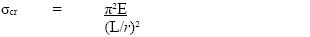
To derive the value of L when critical stress equals proportionate stress, we would put the value of the proportionate stress in the expression
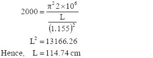
Therefore, till the effective length of the column is 114.74 cm or below, it is not desirable to use the value of critical stress determined from Euler’s formula.
Here we have determined the value of the effective length. It is stated in the problem that the column is fixed at one end and is free at the other. We know that for this condition, the effective column length becomes double of the actual length.
Hence, actual column length for the limiting condition
= 114.74 / 2
= 57.37 cm.
In a way, this reduction in actual length (we can also call it the permissible length for this condition) demonstrates the influence of the end condition on the column.
For this case, we have enough information available to determine the critical stress for any length and end condition. The simplicity of the adopted section has made things very easy for us. However in actual practice, we will come across sections for which it is not very simple to calculate the values of I and A. In such a scenario, it becomes imperative to refer to the manufacture’s data table or the structural engineering codes, to determine this information.
3.12 Conclusion
In this section, we studied the basic principles of strength of materials. We now have an idea about the behavior of materials under various types of stresses. We can also appreciate the reason for these behaviors, the study of which is important from the point of view of structural engineering. We can understand that the presence of a certain physical property or the lack of it, in a given material, is responsible for a certain type of behavior.
We have also studied the mechanism of development of internal stresses under different load conditions and how the physical and geometrical properties influence the same. We have seen the interrelation of different types of stress function (bending and shear), which originates from similar loading. This understanding is going to have wide use in the future, when we will study the design using different materials.
We have seen the phenomenon of deformation of structures under stress and the factors affecting these deformations. We have learnt the principle and procedure of the analysis of the column members, which has its derivation from the principle of deformation.
So far, we have not undertaken the analysis of statically indeterminate structures, which we will take up in the next chapter of this manual.
Learning objectives
After completion of this chapter, one will be able to:
- Understand statically indeterminate structures and determine their degrees of indeterminacy.
- Understand the behavior of the members in statically indeterminate structures
- Understand the effect of physical constraints in statically indeterminate structural systems
- Learn some of the important and widely used analytical techniques and have clarity about their uses and limitations
- Understand the principles that shape the influence lines and their use in the case of statically indeterminate structures
As we are already aware, statically indeterminate structures are those in which the numbers of supports or restraints are more than the minimum essential for maintaining the stability of the structure under loading. The equations of static equilibrium are not enough to derive the values of all the support reactions in the case.
4.1 Structural classification based on the degree of indeterminacy
We have learnt that structures can be classified as structurally determinate or non-determinate, based on the procedure of their analysis. We will further observe the characteristics that lead to this classification.
4.1.1 Statically determinate structures
Structures that can be completely analyzed with the help of statics alone are known as statically determinate structures. The process of finding the reactions in these structures involves the application of the equations of equilibrium. The process needs information on the overall arrangement of the members in the structure and the types of support constraints. At the same time, the process is independent of all other geometric considerations, which means that the determination of internal and external reactions can be done without giving any attention to the deformed shape of the structure.
To explain, a determinate structure can have only as many supports as are absolutely essential for its stability under imposed loading conditions. Thus, a statically determinate structure can also be defined as one in which the number of reactions equals the number of the equations of statics, which are applicable for the particular situation.
4.1.2 Statically indeterminate structures (from chapter 2)
Those structures which cannot be fully analyzed with the help of statics alone are known as statically indeterminate structures. In these cases, the number of unknown reactions exceeds the number of applicable equilibrium equations.
We will consider an example here. Consider the case of a beam AB in Figure 4.1, which is fixed at end A and supported at end B. Structurally, this arrangement is known as the propped cantilever. An inclined load W has been imposed on the beam.
As is obvious from the diagram, there are four unknown support reactions: three at the support A and one at the support B. Only three equations of statics are available (ΣH, ΣV and ΣM = 0). Therefore, the beam AB is a statically indeterminate structure.

Statically Indeterminate and Determinate structures
As we are aware by now, there can only be three possible equations of equilibrium in the case of plane structures. Does it mean that all structures having more than three unknown support reactions are statically indeterminate? Not necessarily. Now consider a modification in the beam of Figure 4.2. Between A and B, a hinge has been installed at C. Clearly, the condition at that moment at C should be equal to zero and provide an additional equation. With this additional equation, it has become possible to analyze all of the four unknown reactions and, therefore, the structure has become statically determinate.
Let us consider another situation for the beam AB. We decide to remove the support at B. The structure would still be stable under the influence of the load W. Simultaneously, it has become statically determinate even without the introduction of any hinge (in fact, in this situation the introduction of a hinge would render it unstable). It can be concluded that the support B was redundant. Therefore, we can say that in a statically indeterminate structure, the number of support reactions is more than those necessary for the stability of the structure. This difference, or alternatively, the number of redundants in the structure, is known as the degree of indeterminacy of the structure.
4.1.3 Determination of degree of indeterminacy
As stated earlier, the degree of indeterminacy is the number of redundant support reactions in a structure, which, on removal, would make the structure statically determinate. Two popular methods to determine the degree of indeterminacy have been explained below. The scope has been confined to plane or two-dimensional structures only.
Cantilever tree method: This method is very useful for rigid jointed frames. Nature has generated examples of some very efficient structural systems, a tree being one such case.
To work out the degree of determinacy for frames by this method, the first step is to ensure that all of the joints should be rigid. This is achieved by providing extra restraints at non-rigid joints (converting them into rigid ones). The number of such restraints is counted (R).
Now, the closed frame structure is cut in such a way that each isolated portion resembles a tree with branches on one or both sides. The numbers of cuts in the total structure are also counted (C).
Degree of indeterminacy = 3×C – R.
We will consider an example of the frame shown in Figure 4.2.

Cantilever tree method to determine the degree of indeterminacy
The frame in the example has two hinged supports. To convert them to rigid, each one has had a single restraint applied:
| Total number of restraints introduced ‘R’ | = 1 + 1 = 2 |
| The number of cuts required to convert into tree ‘C’ | = 6 |
| Hence, degree of indeterminacy | = 3×6 – 2 = 16 |
The underlying principle can be applied to any structure to find its indeterminacy. In the case of indeterminate beams, what is required is to convert any one end of the beam as fixed (if it is not already so) by introducing restraints. Once done, remove all the redundant supports. The degree of indeterminacy can be worked out with the following relationship:
Degree of Indeterminacy = Supports Removed – Constraints Added
Method of joints: This method is more suitable for pin-jointed structures with relatively large number of members. A truss is one example of this type of structure. The principle applied is that each member of the structure has an unknown axial force contributing to the indeterminacy, which is added to the total number of support reactions. Also, each one of the pin joints contributes two numbers of equilibrium equations. Therefore, in the case of a plane structure,
| Degree of Indeterminacy | = Total Members + Total Support Reactions |
| (– 2) × Number of Joints |

Statically determinate truss
Let us take the truss shown in Figure 4.3 as an example for illustration. The truss has a total of 13 members and eight joints. There are two supports: a hinged and a roller. Total support reactions shall be three (two for hinged and one for roller support):
Degree of Indeterminacy = 13 + 3 – 2×8 = 0
The zero degree of indeterminacy indicates that the truss is statically determinate. It may be noted here that if the roller support is converted into the hinged one, the total number of support reactions will increase by one, resultant to which the degree of indeterminacy will become one and the truss will no longer remain statically determinate. The illustrations below would be of help to further understand the procedure.
Illustration 4.1: The frame shown in Figure 4.4 has all the joints rigid. It is needed to determine if the frame is statically indeterminate.

Statically indeterminate frame – illustration 4.1
As we see, the two intermediate supports for the frame are of hinged type. In order to convert them into fixed supports, they need to be provided with one restraint each.
Therefore, Number of Restraints ‘R’ = 2.
Once that done, the frame is a fully rigid one with fixed supports. Now, to convert it into a set of independent cantilever trees, a number of cuts have been introduced in the horizontal members. To find out the number of such cuts required, the diagram of ‘equivalent frame’ is shown in Figure 4.4.
According to this, Number of Cuts ‘C’ = 4.
We know that
Degree of Indeterminacy = 3×C – R
Substituting relevant values,
Degree of Indeterminacy = 3×4 – 2 = 10
Therefore, the frame has the degree of indeterminacy equivalent to 10.
Illustration 4.2: A pin-jointed truss is shown in Figure 4.5. It is needed to determine whether the frame is statically indeterminate.
As we know that for pin-jointed frames, the degree of indeterminacy can be determined from the following expression:
| Degree of Indeterminacy = | Total Members + Total Support Reactions |
| (– 2) × Number of Joints |

Pin-jointed truss – illustration 4.2
| Total Members | = | 17 |
| Total Support Reactions | = | 3 (one at roller & 2 at hinged support) |
| Total Number of Joints | = | 10 |
| Therefore, Degree of Indeterminacy | = | 17 + 3 – 2 × 10 |
| = | 20 – 20 = 0 | |
| This establishes that the truss is statically determinate. |
4.2 Principle of superposition
The superposition is one of the widely used principles in structural analysis. It states that if a structure is under application of multiple loads and the stress–strain relationship follows Hooke’s law, the overall deformation caused by the load system at a particular point shall be equal to the algebraic sum of the deformation caused by the application of each load of the system acting one at a time.
This principle is derived from Hooke’s law. We know that the relationship between the applied force and deformation shall be linear, as long as the material follows Hooke’s law. Let’s assume a force system, consisting of forces F1, F2 and F3, which has been acting on a structure. As shown in the stress–strain relationship in Figure 4.6, the deformations caused by these individual forces are δ1, δ2 and δ3, respectively.
As is obvious from the figure, when we represent the overall force F, as the sum of the individual forces F1, F2 and F3, the corresponding deformation δ shall be equal to the sum of the deformations δ1, δ2 and δ3.

Stress–strain relationship
It is clear that the principle of superposition would not be valid for those cases in which the stress–strain relationship is non-linear. Other circumstances in which it would not be valid are when the application of one force tends to affect the magnitude of another. A case in point is the column subjected to both axial and lateral loads. Here, when lateral load is applied to the column, the resultant deflection of the axis tends to induce an additional moment on the section of deflection. The magnitude of this moment is equal to the product of the axial force and deflection at that point. The value of this moment keeps on increasing with every incremental increase in the lateral force, though the value of the longitudinal force may remain unchanged throughout. When both forces are applied individually, this moment shall not be present in any of the situations.
Here, the cumulative effect of the application of both the forces is not equal to the algebraic sum of their individual applications.
4.3 Analysis of statically indeterminate beams
In addition to the equations of statics, statically indeterminate structural cases require equations that show relationships, between the elastic deformations, in order to derive all the variables necessary for analysis.
For the analysis of statically determinate beams, we will examine two popular techniques. One is the ‘method of superposition’ in which superposition is used for analysis. The other is the ‘method of area moment’.
4.3.1 Method of superposition
This technique of analysis of structures is based on the ‘principle of superposition’. We know that in the case of a statically indeterminate beam, one or more of the support reactions are redundant. Therefore, if the constraints, which are responsible for those reactions, are removed, the beam becomes statically determinate and can be analyzed for those support reactions.
Once that is done, geometrical constraints can then be imposed on the system. These constraints, which relate to either deflection or slope of the elastic curve of the beam, can then be expressed in terms of loads. Such relationships form the additional equations, which are used together with the equations of statics, to determine the values of the support reactions.
To understand it fully, take the case of the beam AB, supported on rollers at A and a hinge at B, as shown in Figure 4.7. The beam has been provided an additional support at C located between A and B. Two concentrated loads, each one in the spans AC and AB, have been acting on the beam. We have two conditions of equilibrium (ΣH = 0 is not relevant in the absence of any horizontal load component). Clearly, the introduction of support C has made one of the support reactions redundant. For the sake of explanation, it is possible to treat either support A or C as redundant; as the beam remains stable if either one is removed.
In this case, we decide to remove support C. The structural arrangement now is statically determinate. The beam under the influence of loads and support constraints would deform as shown in Figure 4.7. Table 4.1 describes expressions for slope and deflection for some standard loading conditions.
If the loading system is different from any standard condition, it is always possible to determine these values with the help of the analytical methods already studied. Let’s say that deflection at point C of the beam in the absence of support is δ1.
In the second step, we remove the imposition of the concentrated loads and place support C back to its original position. The reaction at support C ensures that the beam has no deflection at that point. In other words, the reverse deflection at C due to reaction is equal to the deflection due to imposition of the earlier concentrated loads. Let’s say this deflection is δ2.

Superposition for beam deflection
It is obvious that δ1 is expressed in terms of loads imposed on the beam, whereas δ2 is expressed in terms of reaction at C.
The relation
δ1 = δ2
would provide the magnitude of reaction at C. Once it is known, the reactions at A and B can be determined with the help of relations Σ M = 0 and Σ V = 0.
| BEAM DESCRIPTION | SLOPE | MAXIMUM DEFLECTION | |
|---|---|---|---|
| At End ‘A’ | At End ‘B’ | ||
Cantilever Beam – Span ‘l’
|
Nil | Pl2/2EI | Pl3/3EI |
Cantilever Beam – Span ‘l’
|
Nil | Pa2/2EI | Pa2(3l-a)/6EI |
Cantilever Beam – Span ‘l’
|
Nil | wl3/6EI | wl4/8EI |
Cantilever Beam – Span ‘l’
|
Nil | wl3/24EI | wl4/30EI |
Cantilever Beam – Span ‘l’
|
Nil | Ml/EI | Ml2/2EI |
Simply Supported Beam – Span ‘l’
|
Pl2/16EI | Pl2/16EI | Pl3/48EI |
Simply Supported Beam – Span ‘l’
|
Pb(l2-b2) /6lEI | Pab(2l-b) /6lEI | Pb(l2-b2)3/2/9√3lEI at √{(l2-b2)/3} from end A |
Simply Supported Beam – Span ‘l’
|
wl3/24EI | wl3/24EI | 5wl4/384EI |
Simply Supported Beam – Span ‘l’
|
7wl3/360EI | wl3/45EI | 0.00652wl4/EI at 0.519l from A |
Simply Supported Beam – Span ‘l’
|
Ml/6EI | Ml/3EI | Ml2/9√3EI at l/√3 from A |
To illustrate the technique, the analysis of a propped cantilever beam has been demonstrated below.
Illustration 4.3: The propped cantilever AB has been fixed at A and supported at B. The beam has a span of 6 m and a uniformly distributed load of 600 N/m is acting on the entire span of the beam. The arrangement is shown in Figure 4.8.
Firstly, we use the equilibrium equations applicable to the situation. As per these,
Σ V = 0 and Σ M = 0.
Hence,


Propped Cantilever – Bending moment diagram- illustration 4.3
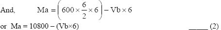
If we assume the case when support B is not present and the beam AB is a normal cantilever, the downward deflection at end B due to the imposed load shall be expressed as follows:
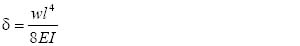
Also, if we consider the situation when reaction at B is the only applicable load on the beam, the upward deflection in the beam due to reaction at B shall be expressed as follows:
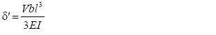
As there has been no net deflection at point B, the following relation emerges from the principle of superposition:
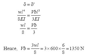
By substituting this value of Vb into equation (1),
| Va + 1350 = 3600 | |
| Hence, | Va = 2250 N |
Similarly, putting the value of Vb into equation (2),
Ma = 10800 – 1350×6
Ma = 2700 N.m
By this way, magnitudes of all the support reactions have been determined.
It may be worth noticing the effect of providing a prop at the free end of the cantilever. The moment at fixed end, which would have been 10800 N.m in the absence of the prop, has come down in the case by 75% to 2700 N.m.
4.3.2 Method of area moment
We already know that in the case of statically indeterminate beams, it is always possible to define some constraints of slope or deflection somewhere along the span. These constraints lead to certain conditions, which can be expressed mathematically with the help of the moment area theorems, described in Section 4.6. These expressions, along with the equations derived from statics, can be solved simultaneously to get the values of support reactions.
To further clarify, take the example of a beam AB of span l, built-up in the supports at both the ends. The beam has had two concentrated loads applied, W1 and W2, which are acting vertically downward. The arrangement is shown in Figure 4.9.
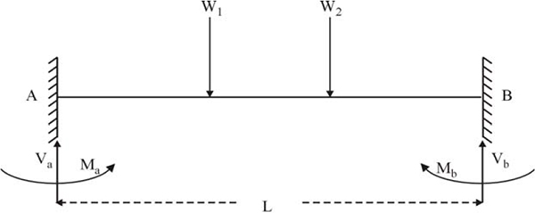
Fixed ends beam- support reactions and moments
Under the influence of this load system, the support reactions generated are Va, Ma, Vb and Mb.
From the condition of equilibrium, we derive the following two equations:
| Va + Vb = W1 + W2 | |
| and | Ma= Mb – Vb×l + W1×l1 + W2×l2 |
It is clear that four unknowns cannot be determined with the help of the two equations. Hence, we would go further and identify some critical constraints of the system. There can be three such constraints.
The ends A and B would not allow any rotation, due to which the tangents drawn at both the points in the elastic curve would be parallel (in fact, tangents would coincide as A and B are at the same level with respect to the horizon). Therefore, the angle between A and B is nil. We know from the first moment area theorem that the angle between two points is equal to the area of the bending moment diagram between these points, divided by EI.
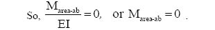
As the tangents on points A and B of the elastic curve are parallel to each other, the deviation at A from tangent drawn at B would be equal to zero. Similarly, the deviation at B from the tangent drawn at A would also be equal to zero. From the second moment area theorem, such deviation shall be equal to the moment of the bending moment diagram about A and B respectively, divided by EI:
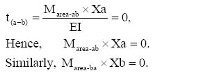
In all these expressions, the values shall be expressed in the form of imposed loads, span and reactions. With the help of one of these two equations, along with the two equations earlier derived from statics, it is possible to determine the value of all the four unknowns.
We will demonstrate the application of area–moment method with the help of the following illustration.
Illustration 4.4: The beam AB has both the ends A and B rigidly fixed. The beam has a span of 9 m and a concentrated load of 5000 N is acting at point C, located 3 m away from B. The arrangement is shown in Figure 4.10.
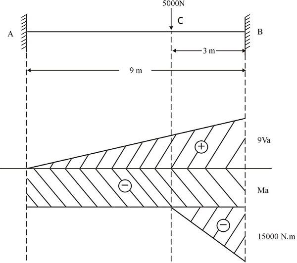
Bending moment diagram- illustration 4.4
There are four unknowns in the arrangement, which are Va, Ma, Vb and Mb.
Firstly, we use the equilibrium equations applicable to the situation. As per these,
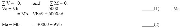
Further to apply the area–moment method, we would draw the bending moment diagram ‘by parts’ as explained previously in the application of moment–area theorems. Considering B as the fixed end, the bending moment diagram is shown in Figure 4.10.
Due to the rigidity of the fixed ends, there would be no rotation permitted and the tangents at the elastic curve at these two points shall be parallel. In this situation, the angle between these two points would be zero. According to the first moment–area theorem, the area of the bending moment diagram between A and B also shall be equal to zero:
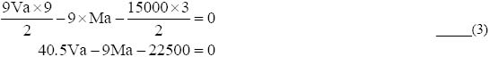
Also, since the tangents are parallel and at the same level at A and B, the deviation at B with the tangent drawn at A would be zero. From the second moment area theorem, the bending moment diagram between A and B with respect to B shall be equal to zero:
t(a-b) = Marea-ab×xa = 0
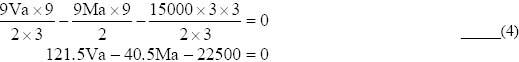
Solving equations (3) and (4) simultaneously, we get
Va = 1296.3 N and Ma = 3333.35 N.m
Putting the value of Va into equation (1),
Vb = 3703.7 N
Putting the values of Ma and Vb into equation (2),
Mb = 6666.65 N.m
4.4 Multispan or continuous beams
Till now, we have observed the analysis of beams, which had one or at the most two spans. If the beam has a larger number of spans, it is still possible to use any of the above-described methods for analysis. However, the number of simultaneous equations increases with the number of redundants in the beam. This increases the complexity of the procedure. A more convenient way would be to first determine the magnitude of the moments at the supports. Determining the support reactions would be a subsequent step. We will examine one such method in the section.
4.4.1 Three-moment equation
In the three-moment equation, a general relation between bending moments at any three sections of a beam is established. It is a relationship between the moments at those sections, distances between them and the deflection of the elastic curve at those points. Since the reaction moments are more critical in the case of a multispan beam, the sections chosen for application of the three-moment equation can be three consecutive supports.
The expression of three-moment theorem is as follows:
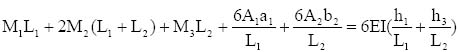
Here,
| M1, M2 and M3 | = | Moment at Section – 1, 2 and 3 respectively |
| L1 | = | Distance between Section – 1 and 2 |
| L2 | = | Distance between Section – 2 and 3 |
| A1 | = | Area of bending moment diagram between Section – 1 and 2 |
| a1 | = | Moment arm of A1 with respect to Section – 1 |
| A2 | = | Area of bending moment diagram between Section – 1 and 2 |
| b2 | = | Moment arm of A2 with respect to Section – 3 |
| h1 | = | Height of point 1 of the elastic curve with respect to point 2 |
| h3 | = | Height of point 3 of the elastic curve with respect to point 2 |
Normally when we consider a horizontal beam and apply the three-moment theorem to any three non-yielding supports, those that are not subjected to settlement, the values of h1 and h3 become zero. In such case, the three-moment equation assumes a relatively simple form, which is
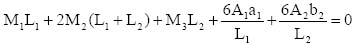
To simplify the procedure further, it is helpful to always select at least one support for which the value of the moment is determinable. For instance, if the end supports are not fixed, the value of the moment there shall be zero. Also if there has been an overhang beyond one of the end supports, the value of the moment at this support due to loading at the overhang portion can be determined easily.
4.4.2 Determination of shear force from moment diagram
We have observed the procedure of direct determination of moment at the beam sections. The application of the three-moment equation can provide the value of moments at the sections or supports. However, it does not directly provide the magnitude of the support reactions. It is crucial to know the support reactions in order to determine the shear force at different sections of the beam.
To determine the support reactions, the below procedure is required to be followed. Figure 4.11 should be referred in order to understand the steps involved.
M = M1 – M2
- Isolate the beam span and represent it as a free body with all the imposed loads. Suppose the length of the span is L. The moments as determined by the analysis should be indicated as acting on both the ends.
- The support reactions, which are unknown, would also be shown as acting on both the supports.
- To determine the magnitude of support reactions, the diagram would be further resolved into two independent ones. The first one would show the external loads imposed sans support moments and the reactions as applicable in the case of a simply supported beam.
- The second diagram would show the imposition of moments M1 and M2 at both the ends. Assuming that both the moments would not be equal (and they actually would not be on most of the occasions), the net moment acting on the span would be equal to
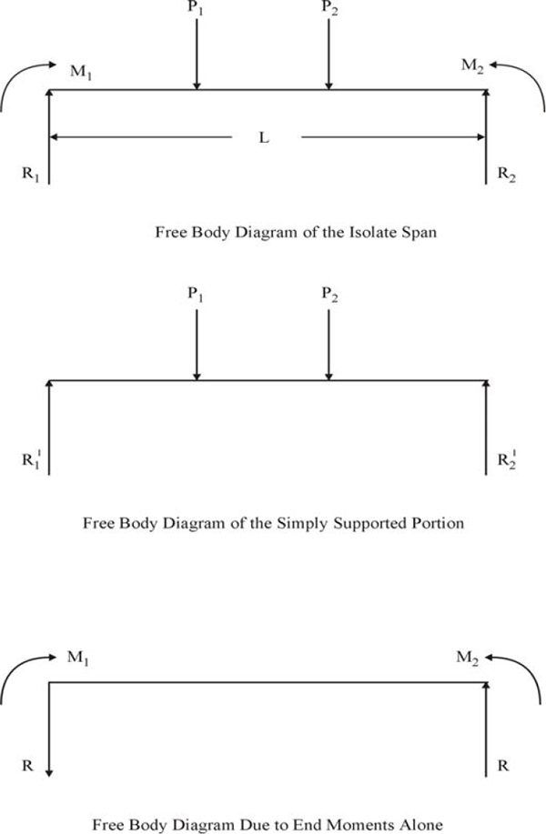
Shear force determination
The moments M1 and M2 would be given the proper signs as applicable in a particular case. Here it is assumed that both are positive and M1 > M2.
Since M1 is assumed to have larger magnitude, its overall effect would be to rotate the beam in a clockwise direction. For equilibrium, the reactions at both the ends would form a moment couple of equal magnitude, acting anticlockwise.
If the force of the couple is R, the magnitude of the couple would be R×L, as L is the arm of the couple.
In the state of equilibrium,
R×L = M1 – M2
Hence, 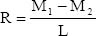
Therefore, the magnitude of the reaction would be similar for both ends. The only difference being that it would act downward at end 1 and upward at end 2.
- The net reaction at ends 1 and 2 would be the algebraic sum of the reaction due to applied load and the reaction due to moment’s application.
- The shear force diagram would now be drawn in the usual way by starting from an end.
This procedure of drawing the shear force diagram is very useful for the statically indeterminate structures with a high degree of indeterminacy. Besides beams, the method can be applied to any type of structure. The same procedure would be used to draw shear force diagrams for frames, as we would see in the further sections.
4.4.3 Determination of shear force
As we have seen earlier, the reaction at a particular support shall be the algebraic sum of the reaction due to loads imposed and the reaction due to moment differential at the two supports. This would be equal and opposite at both the supports to form a resisting couple. We also know that the value of this reaction would be
To make it easy to calculate, the values of both these components for each support reaction are shown in Figure 4.12 and, thus, the net reaction for each support has been worked out. These values have been used to draw the shear force diagram, which is also shown in Figure 4.12.
To illustrate the application of the three-moment theorem to determine the support moments and utilization of the results to determine the shear force diagram, we will look at the following situations.
Illustration 4.5: The beam ABC has ends A and C simply supported and is continuous over the support B. The spans and the loads imposed are shown in Figure 4.12. We have to determine the bending moment at critical locations and draw the moment diagram.
To start with, we would apply the three-moment theorem to the set of supports A, B and C. As the supports are non-yielding, h1 and h3 would be equal to zero. As is obvious, the magnitude of the moment at the end supports A and C would be equal to zero. Also, in view of second span having no load on it, the moment in bending moment diagram would also be zero. The applicable relationship equation would be
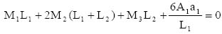
To determine the value of the expression A1a1, we need to draw the bending moment diagram for the load on the span AB. Refer to Figure 4.12, where bending moment diagram in parts for span AB has been drawn. It has been drawn in this way to make it easy to calculate the moment of the area about A, the first section. The ordinates to calculate the area have also been indicated in the diagram.
Therefore,
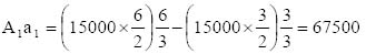
Substituting this value along with others (M1, M3 = 0) into the three-moment equation,
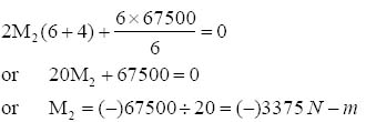
Therefore, the value of moment at support B is (–) 3375 Nm. In order to draw the bending moment diagram, we also need to derive the bending moment due to load applied.
Considering span AB, the reaction due to load would be 2500 N on each support.
Mid span moment = 2500 x 3 = 7500 NM.
Using these values of moment, the overall bending moment diagram is shown in Figure 4.12.
Now, in order to determine the shear force, let’s consider both the spans separately.
Span AB
The support moment at A is zero and at B is 3375 NM.
Hence, net moment = 3375 NM.
The moment has tendency to rotate the span in a clockwise direction. The anti-clockwise couple of reaction R1 would resist this.
From this, the value of reaction R1 = 3375/6 = 562.5 N.
Span BC
Similarly for span BC, the support moment at C is zero and at B is 3375 NM.
Hence, net moment = 3375 N-m.
The moment has tendency to rotate the span in an anti-clockwise direction. The clockwise couple of reaction R2 would resist this.
From this, the value of reaction R2 = 3375/4 = 843.75 N.

Continuous beam – illustration 4.5
The combined effect of the reactions due to vertical load and moments is shown in Figure 4.12, along with the resultant shear force diagram.
Illustration 4.6: The beam ABCD has both the ends A and D simply supported and is continuous over the supports B and C. All the supports are non-yielding types. The spans and the loads imposed are shown in Figure 4.13. The objective is to draw the bending moment and shear force diagram for the beam system.
First of all, we would apply the three-moment theorem to the set of supports A, B and C. Since the supports are non-yielding, the values of h1 and h3 would be zero. Also, the magnitude of the moment at the end support A would be equal to zero and since the first span has no load on it, the moment of bending moment diagram would also be zero. The applicable relationship equation would be
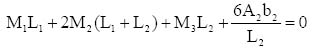
To determine the value of the expression A2b2, we would draw the bending moment diagram for the load on the span BC. Since moving further we need the values of similar expression for the next span also, we would draw the bending moment diagram for span CD, too. Refer to Figure 4.10(a), in which bending moment diagram in parts for span BC has been drawn. It has been drawn in this way to make it easy to calculate the moment of the area about C, the third section. The ordinates to calculate the area have also been indicated in the diagram.
Hence,
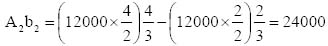

Bending Moment Diagram for a continuous beam- illustration 4.6
Substituting this value along with others into the three-moment equation,
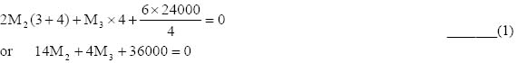
Similarly, when we consider sections B, C and D for the application of the three-moment theorem, the applicable expression shall be as follows:
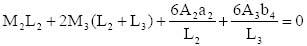
To calculate the values of A2a2 and A3b4, we will refer back to Figures 4.13. It may be noted that the bending moment diagram for span BC in 4.13 is essentially similar to the one drawn below it, but has been drawn in such a way to make it easier to calculate its moment about B, which is the requirement this time.
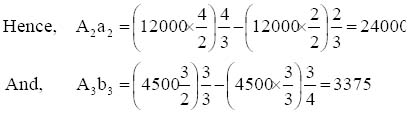

Bending moment and shear force diagrams- illustration 4.6
Substituting all the values into the expression,
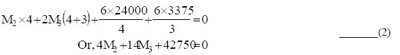
Solving equations (1) and (2) simultaneously,
| M2 | = | (–) 1850 NM | |
| and | M3 | = | (–) 2525 NM |
The resultant bending moment diagram is shown in Figure 4.14. Also have been derived the shear force diagram, adopting the procedure explained under illustration 4.5.
4.4.4 Deflected shape of the beam
The deflected shape of the beam or the elastic curve is interesting to determine. We know that the sign of bending moment determines the type of curvature of the elastic curve at a section. To know the net value of the bending moment at a particular section, the positive moment diagram has been superimposed on the negative moment diagram. The common area of both does cancel each other and the portion remaining represents the net bending moment diagram. On observing this net bending moment diagram, it is clear that the value of bending moment remains negative throughout the spans AB and CD. Therefore, the shape of the elastic curve would be concave upwards for both these spans. In the middle span BC, the value of bending moment changes the sign at two points, I1 and I2. Obviously, these are the points of inflexure. Also, the values of the bending moment remain positive between these two points. Hence, the elastic curve shall remain concave downwards between these two points.
4.5 Slope-deflection method
Once we move to cases of indeterminate structures, where instances like yielding of supports, rotation and deflection of joints, geometrical arrangements other than a linear beam, etc. are involved, it becomes quite complex to use any of the earlier described method. For such situations, there are a few more good techniques available.
The slope-deflection method is one such technique. Here, the main assumptions used to write the equations are as follows.
- First of all, the joints of structural members are assumed rigid. Therefore, if the joints were not restrained against rotation, they would rotate in such a way that the angle between the members emanating from a joint would remain unchanged after the rotation.
- In a structural system, the algebraic sum of the end moments of the members, meeting at a joint, which is free to rotate, would always be equal to zero.
In the slope-deflection method, the end moments are expressed in terms of slope and deflection at the ends of the members.
4.5.1 Derivation of the slope-deflection equation
While writing an equation the following sign conventions are followed:
- Clockwise moments are designated as positive and anticlockwise as negative.
- Clockwise angles of rotation are expressed as positive and anticlockwise as negative.
- The deflection responsible to rotate the member clockwise is treated as positive and the one, which rotates anticlockwise, is treated as negative.
To derive the slope-deflection equation, consider the case of the beam AB of length L, as shown in Figure 4.15(a). Suppose the ends are free to rotate for the beam. A set of traverse loads has been applied to the beam, which has not been shown in the diagram for the sake of simplicity.
Due to influence of these loads, the net values of moment at A and B are MAB and MBA respectively. The angles of rotation of both the ends are θA and θB respectively. In addition, the end B has undergone a lateral deflection of magnitude δBA with respect to end A.
It is clear that this entire arrangement can be divided into following components.
- A beam with both the ends fixed has all the transverse loads applied to it. The same is shown in Figure 4.15(b). The beam has been subjected to the fixed end moments of magnitudes MFAB and MFBA.

Slope-deflection relationship for a beam
- A beam has end B fixed and A simply supported with no lateral loads, but subject to moment M’A at end A. This is shown in Figure 4.15(c). The moment has induced a rotation of θA at A, whereas B is unaffected. The resultant moment at B would be M’B.
- A beam has end A fixed and B simply supported with no lateral loads, but subject to moment M’’B at end B. This is shown in Figure 4.15(d). The moment has induced a rotation of θB at B, whereas A is unaffected. The resultant moment at B would be M’’A.
- Fixed beam with no lateral loads, but subject to a deflection of magnitude δBA of end B with respect to end A. This is shown in Figure 4.15(e). The induced moments due to it are M’’’A and M’’’B respectively.
The sum of these four would geometrically and statically be equivalent to the original beam system.
| Hence, | MAB | = | MFAB + M’A + M’’A + M’’’A. |
| And | MBA | = | MFBA + M’B + M’’B + M’’’A. |
Let us proceed to determine and express the values of end moments in the form of deformations.
The fixed end moments MFAB and MFBA are the function of the loads imposed on the member and its length.
For cases 2 and 3, the value of the moment at the end of rotation would be equal to 4Eiθ/L, whereas for the fixed end the value of the moment would be equal to 2Eiθ/L.
Therefore, in case 2,
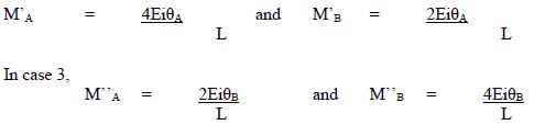
For the fourth case, where deflection has been inducing the moments at both the ends, the magnitude of such moment would be equal to 6Eiδ/L2.

It may be noted here that the direction of the moment at both the ends would be anti-clockwise (hence negative sign), whereas the rotation of the member itself has been positive. Substituting these values into the moment relationships,
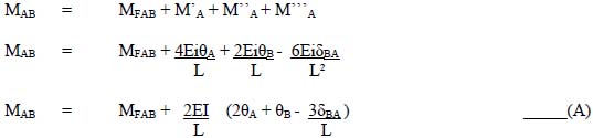
In the same way,

Equations (A) and (B) are slope-deflection equations. The expression δ/L in them is sometimes referred to as the rotation of the member.
4.5.2 Calculation of fixed end moment
The calculation of fixed end moments, required in the equations, could be time-consuming. To make it faster, the expressions to determine the values of the fixed end moment, for some standard loading conditions, have been provided in Table 4.2. It may be noted that the table provides only the absolute values and the sign of the moment has to be decided according to the situation in the problem.
| Load Description for Fixed Beam of Span ‘l’ | Fixed End Moment | |
|---|---|---|
| At End ‘A’ | At End ‘B’ | |
| Point Load ‘P’ applied at mid span | Pl/8 | Pl/8 |
| Point Load ‘P’ applied at distance ‘a’ from A and ‘b’ from B | Pab2/l2 | Pa2b/l2 |
| Uniformly Distributed Load ‘w’ per length applied throughout the span | wl2/12 | wl2/12 |
| Uniformly Varying Load ‘w’ per length at A to zero at B applied on the span | wl2/20 | wl2/30 |
| Uniformly Varying Load ‘w’ per length at the centre the span to zero at A and B both | 5wl2/96 | 5wl2/96 |
| No external load application but the relative movement ‘d’ between the two fixed ends of the beam | 6EId/l2 | 6EId/l2 |
4.5.3 Application of slope-deflection equations
The stepwise application of the slope-deflection equation to analyze a structure, in its general form, is as follows:
- First of all, consider all the joints as fixed and calculate the fixed end moments for the nodes.
- For each span of the structure, express both the end moments in the form of deformations using slope-deflection equations.
- Establish the equation for moment equilibrium of each joint, which is free to rotate. For equilibrium conditions, the algebraic sum of the end moments of all the members of the joint would be equal to zero.
- In the case of any other deformation like side sway or settlement, the additional equilibrium equation for stability would also be arrived at.
- Calculate the values of the deformations by solving the above equations simultaneously.
- All such calculated values of deformations would be substituted into the equations to determine the values of the moments.
The illustration below will be useful to understand the procedure better.
Illustration 4.7: The beam ABC has ends A and C simply supported and is continuous over support B, which is non-yielding. The spans and the loads imposed are shown in Figure 4.16.

Bending moment diagram for beam – illustration 4.7
First of all, we shall consider all the joints as fixed and calculate the end moment for each span, resultant to the imposed loading:
| MFAB | = | MFBA = | 0 (Since no external load) |
| MFCB | = | (-)MFBC = | wL2/12 = 1000×62/12 = 3000 NM |
In the next step, we would write the slope-deflection equation for each joint. The basic equation is
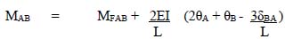
For joint A, the values of MFAB, and ΔBA would be zero.
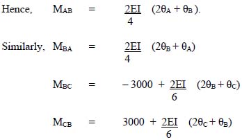
In the above equations for moment, it is clear that the second expression on right-hand side is the multiplication of the angles of rotation of joints, with the value equivalent to 2EI/L. Since we are not interested in determining the value of the individual angles of rotation, it is okay if we assign some arbitrary value to EI, which makes it convenient for our further calculations. The ultimate values derived for the angles would be perfectly okay when used in combination with this value of EI.
In this particular case, let us assign a value of 6 to EI.
| Now, | MAB | = | 6θA + 3θB |
| MBA | = | 3θA + 6θB | |
| MBC | = | – 3000 + 4θB + 2θC | |
| MCB | = | 3000 + 4θC + 3θB |
The next step is to write the equilibrium equations for the joints, where a clear relationship emerges.
These equations are
| MAB | = 0 | |
| MBA + MBC | = 0 | |
| And, | MCB | = 0. |
Substituting derived values of the moments in these condition equations, we get
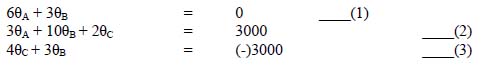
We now need to solve equation (1), (2) and (3) simultaneously to determine the values of three unknown angles.
| From equation (1), θA | = | (-)θB / 2 |
| From equation (3), θC | = | -750 – 3θB / 4 |
Substituting these values into equation (2),
| -3θB / 2 + 10θB – 1500 – 3θB / 2 | = | 3000 |
| θB | = | 642.85 |
| From this, θA | = | (−)321.43 |
| θC | = | (−)1232.14 |
Substituting these values of slope to derive the fixed end moments,
| MAB | = | 0 |
| MBA | = | 3θA + 6θB |
| = | 3 x ( −321.43) + 6 x 642.85 | |
| = | 2892.8 NM | |
| MBC | = | – 2892.8 NM |
| MCB | = | 0 |
The resultant bending moment diagram is shown in Figure 4.15.
In order to bring further clarity, we once again shall solve the example of continuous beam of Illustration 4.6, which previously has been solved by using three-moment theorem.
Illustration 4.8: The beam ABCD has both the ends A and D simply supported and is continuous over the supports B and C. All the supports are non-yielding type. The spans and the loads imposed are shown in Figure 4.16.
In the first step, we shall consider all the joints as fixed and calculate the fixed end moment at the end of each span, due to the imposed loading:
MFAB = MFBA = 0
| MFCB | = | (−)MFBC | = | WL/8 | = | 5000×4/8 | = | 2500 NM |
| MFDC | = | (−)MFCD | = | wL2/12 | = | 1000×32/12 | = | 750 NM |
In the next step, we would write the slope-deflection equation for each joint. The basic equation is

For joint A, the values of MFAB and ΔBA would be zero.


Bending moment and shear force diagram- illustration 4.8

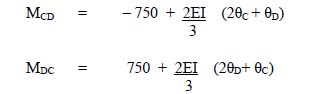
For this case, we assign a value of 6 to EI.
| Now, | MAB | = | 8θA + 4θB |
| MBA | = | 4θA + 8θB | |
| MBC | = | – 2500 + 6θB + 3θC | |
| MCB | = | 2500 + 6θC + 3θB | |
| MCD | = | –750 + 8θC + 4θD | |
| MDC | = | 750 + 8θD+ 4θC |
The next step is to write equilibrium equations for the joints where the relationship is clear.
These equations are
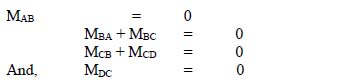
Substituting the derived values of the moments into these condition equations, we get

We are now required to solve equations (1), (2), (3) and (4) simultaneously to find the values of all the four unknown angles. For this, we would need to perform the Gauss–Seidel iteration. This would require us to rewrite the above equations in the following forms:

Setting θB = 0 in equation (1),
θA = 0
Setting θA = 0 and θC = 0 in equation (2),
θB = 178.57
Setting θB = 178.57 and θD = 0 in equation (3),
θC = –163.21
Setting θC = –163.21 in equation (4),
θD = –12.15
A number of such cycles of iteration would require to be performed, by setting the previously obtained values, till we obtain two consecutive sets of values, which are almost similar to each other. The results of this exercise are shown in Table 4.3.
| Cycle | θA | θB | θC | θD |
|---|---|---|---|---|
| 1 | 0 | 178.57 | –163.21 | –12.15 |
| 2 | –89.3 | 239.7 | –172.8 | –7.35 |
| 3 | –119.9 | 249.8 | –176.4 | –5.55 |
| 4 | –124.9 | 252.0 | –177.3 | –5.1 |
| 5 | –126.0 | 252.5 | –177.6 | –5.0 |
The set of simultaneous equations can be solved by any other technique also. The Gauss–Seidel iteration is one of the popular techniques for the solution of simultaneous equations in case the number of unknown exceeds three.
Since the differences in the values obtained in the fourth and fifth cycles are nominal, we would adopt the values of the fifth cycle as a solution to these equations.
By substituting these values of slopes, the values of end moments are as follows:
| MAB | = | 0 |
| MBA | = | 1517 NM |
| MBC | = | – 1517 NM |
| MCB | = | 2192 NM |
| MCD | = | – 2192 NM |
| MDC | = | 0 |
The bending moment diagram, shear force diagram and the deformed shape (dotted lines) of the beam are shown in Figure 4.16.
4.5.4 Application of slope-deflection equations for frame analysis
The slope-deflection method is the major application in the analysis of frames. The frames are the structure, which is formed of vertical and horizontal (sometimes inclined too) members. A typical frame in RCC (reinforced cement concrete) is shown in Figure 4.17.
In our case, we are only considering frames with rigid joints. These joints are capable of rotation as a whole, but the angles between the members at a joint remain unaltered.

Typical RCC framed structure
In the case of frames, unlike beam junctions, the joints can be unrestrained and therefore can shift from their original positions under loading. Since we are considering two-dimensional frames with load application in the same plane, the shift or the movement of joints would remain inter-plane. This shift is termed as sway.

Frames – types and loadings
Coming back to frames, these are of two types. One has symmetry about some vertical axis. Apart from similar geometry on both sides of the axis, the corresponding members would also have the same sectional properties and end conditions. Frames meeting this criterion are known as symmetric frames. All others are known as the anti-symmetric frames.
Similarly, load applications can also be symmetric or anti-symmetric in nature.
Some examples of symmetric and anti-symmetric frames, as well as symmetric and anti-symmetric loadings are shown in Figure 4.18.
While analyzing the behavior of the frame under loading, we need to remember that the frames may or may not be subjected to sway. The sway-related behavior of the beam for different combinations of frames, loadings and restrains has been described in Table 4.4.
| Type of Frame | Type of Loading | Joint Condition | Result |
|---|---|---|---|
| Symmetric | Symmetric | Unrestrained | No-sway |
| Symmetric | Symmetric | Restrained | No-sway |
| Symmetric | Non-symmetric | Unrestrained | Sway |
| Symmetric | Non-symmetric | Restrained | No-sway |
| Non- symmetric | Symmetric | Unrestrained | Sway |
| Non- symmetric | Symmetric | Restrained | No-sway |
| Non- symmetric | Non -symmetric | Unrestrained | Sway |
| Non- symmetric | Non -symmetric | Restrained | No-sway |
It is clear that the condition of non-symmetry either of frame or of loading is sufficient to make the frame sway, provided there has been no physical restraint against it.
If it can be recollected, we already have discussed the effect of restraint on a frame in Section – 2. It is obvious that the flexural behavior of the members of the same frame can be very different in the sway and no-sway conditions.
Analysis of frames meeting ‘no-sway’ condition
For frames with no-sway, the procedure of analysis is similar to the one we have followed in the analysis of the continuous beam. It involves steps like calculations of fixed end moment, writing slope-deflection equations for each span, defining conditions of constraints and solution of resultant equations simultaneously.
The following illustration should make the procedure amply clear.
Illustration 4.9: The frame ABCD has both the ends A and B fixed, and C and D free. The spans, loads imposed and relative moment of inertia for each member are shown in Figure 4.19.
In the first step, we shall consider all the joints as fixed and calculate the fixed end moment at the end of each span, due to the imposed loading:
MFAC = MFcA = 0
MFDC = (–)MFCD = WL/8 = 10000×6/8 = 7500 NM
MFDB = (–)MFBD = 0

Bending moment and shear force diagrams- illustration 4.9
In the next step, we would write the slope-deflection equation for each joint. The basic equation is
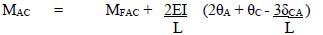
Here, the values of deflection at C and rotation at A are zero.

Let us assign a value of 6 to EI:

The equations of constraints are as follows:
MCA + MCD = 0
And, MDC + MDB = 0
Substituting the values of moments into these relation equations, we get

On solving equations (1) and (2) simultaneously, we get the following values:
θC = 750
And, θD = (–)750
Substituting these values of θC and θD, we derive following values of end moments:
MAC = 2250 NM
MCA = 4500 NM
MCD = (−) 4500 NM
MDC = 4500 NM
MDB = (−) 4500 NM
MBD = (−) 2250 NM
The resultant bending moment diagram is shown in Figure 4.19.
To draw the shear force diagram, the previously described method of drawing free-body diagrams for individual members shall be used to determine the reactions.
For member AC,
| Net Moment | = | 2250 +4500 | = 6750 NM (Clockwise) |
| Shear Force | = | 6750 / 4 | = 1687.5 N |
Span AC has no other force acting on it; hence, the values determined above shall be the net reaction force acting at the nodes.
For member CD,
| Net Moment | = | –4500 +4500 | = 0 |
| Shear Force | = 0 |
A concentrated load of 10000 N has been acting on the centre of the span CD. Due to it, each support shall offer a reaction of 5000 N.
For member CB,
| Net Moment | = | − 2250 − 4500 | = 6750 NM (Anticlockwise) |
| Shear Force | = | 6750 / 4 | = 1687.5 N |
Span CB has no other force acting on it; hence, the values determined above shall be the net reaction force acting at the nodes.
The resultant shear force diagram is shown in Figure 4.19.
Analysis of frames subjected to ‘sway’
For frames, which are subjected to side sway either due to anti-symmetric configuration or loading or both, the process of analysis includes the accounting for the sway in the slope-deflection equations.
For this, the direction of sway and its relative magnitude are assessed for each member. Mostly, it is easy to determine the direction of the sway based on the load configuration. Even if the direction were assessed opposite to the actual one, the ultimate sign of the value derived would help in making the required correction.
The other important addition in the procedure is the introduction of the shear equation, as one of the condition equations. This is derived by applying the condition of horizontal stability to the entire frame. According to this condition,
ΣH = 0
For this, the net horizontal reactions on each member are expressed in the form of the sum of the end moments, divided by member length. The cumulative reaction of these net horizontal reactions added with direct horizontal force is expressed equal to zero.
So, ΣH = H1 + H2 + .. + (MAB + MBA)/LAB + (MCD + MDC)/LCD + = 0
To clarify the procedure, we solve a simple case in the illustration below.
Illustration 4.10: The frame ABCD has both the ends A and B fixed, and C and D free. The spans, load imposed and relative moment of inertia for each member are shown in Figure 4.20.
It is very clear that due to the load imposed on joint C, there would be a lateral sway in the frame. The location of the joint C and D would shift to the right, consistent with the direction of the application of load at C. The new positions assumed by C and D would be C’ and D’ respectively. Let us assume that the magnitude of sway of the joint C to its new position C’ is δ. Since the lengths of the member can be assumed to remain unchanged due to loading, the corresponding sway at D would also be equal to δ in magnitude.
All the three members of the frame have no load applied between the nodes; hence, the fixed end moments for all the cases would be zero.
Therefore, MFAC = MFcA = 0
MFDC = MFCD = 0
MFDB = MFBD = 0
In the next step, we would write the slope-deflection equation for each joint. The basic equation for member AB is

In this case, the values of MFAC and θA are zero. Also, the relative deformation of the joints is such that the member rotates in a clockwise direction. Hence, the magnitude of δCA would also be considered positive and the expression 3δ/L would retain its original negative sign.

By substituting an arbitrary value of 2 for the expression EI, we get

In the same way,
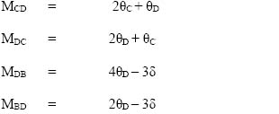

Bending moment and shear force diagrams – illustration 4.10
The conditional equations for this case are
MCA + MCD = 0
MDC + MDB = 0
And the shear equation is
5000 + (MAC + MCA)/LAC + (MDB + MBA)/LDB = 0
Substituting the values,

By solving equations (1), (2) and (3) simultaneously, we obtain the following values:
θC = 74.6, θD = 559.68 and δ = 1144.23
Substituting these values into the end moment equations,
| MAC | = | (–) 783.57 NM, MCA | = | (–) 708.9 NM, |
| MCD | = | 708. 9 NM, MDc | = | 1193.96 NM, |
| MDB | = | (–) 1193.96 NM, MBD | = | (–) 2313.33 NM |
To draw the shear force diagram, we need to determine the end reaction of each member. In this case, apart from the load at node C, no external load has been acting on the span of any member. Any load at the node does not induce shear force; hence, the shear force generation would only be due to the end moments.
For span AC,
| Rac = Rca | = | − (783.57 + 708.9)/ 4 | = 373.1 N (clockwise couple) |
| Rcd = Rdc | = | (708.9 + 1193.96)/ 4 | = 475.7 N (anticlockwise couple) |
| Rdb = Rbd | = | − (1193.96 – 2313.33)/ 2 | = 1753.64 N (clockwise couple) |
The bending moment and shear force diagrams are shown in Figure 4.20.
The above illustration makes clear the method of application of shear equation to solve structural situations, where sway of the frame is involved.
The slope-deflection method can similarly be used to solve structural problems pertaining to multibay frames (frames with more than one span), multistoried frames or frames with inclined members. The advantages of the slope-deflection method are given below:
The method has been derived from the basics and in turn can be used as a basis for other techniques.
It can be used to solve any type of structural problem.
The results derived are quite accurate.
The technique however, has a disadvantage. The number of linear simultaneous equations required to derive a complete solution is equal to the number of unknowns. When increasing the number of structural nodes, the number of the equations can become quite large. This does make the solution complex and cumbersome. In such a situation, it becomes imperative to use some ‘stand-alone’ iteration technique to solve the large number of simultaneous equations. This disadvantage of the technique has been overcome in the ‘moment-distribution method’.
4.6 Moment-distribution method
In the moment-distribution method of structural analysis, the joint equilibrium equations, already described in the slope-deflection method, are solved, without writing them explicitly. In this method, each of the joints is released one at a time instead of releasing all of them together as in the slope-deflection method. The iteration of values is done at each such step. This technique involves a tabular form of calculations, which makes it much simpler compared to the solution of slope-deflection equations.
The concepts and fundamentals of the technique have been described below.
4.6.1 Rotational stiffness of the member
Let’s consider the case of a member AB of length L. The member has a prismatic section and its moment of inertia is I. A moment of magnitude MAB has been applied at the joint A. The joint A is free to rotate and the rotation of the joint due to the application of the moment is θA. On the other end, the joint B can have either of the following two conditions.
First Situation: End B is fixed and unable to rotate
In this situation, the introduction of moment MAB at A would induce a moment MBA at B such that the rotation at B becomes zero. This situation can be described as follows.
- End B is on hinge and subjected to a rotation equivalent to θ’B due to the application of moment at A. In this situation, the rotation at A itself is equivalent to θ’A.
- End B is subjected to a moment MBA due to which the rotation at B becomes θ’’B. This moment does induce θ’’A rotation at A.
These situations are shown in Figure 4.21.
This way, the net rotation at B would be zero. At A, the net rotation is the algebraic sum of the rotations induced in both the situations.
Hence, θA = θ’A – θ’’A.
And θB = 0 = θ’B – θ’’B.

Moment-distribution: rotation of member
In the first case, when A is subjected to moment MAB, the values of rotations at A and B would be the following:

Similarly, due to induction of moment MBA at B the values of rotations at A and B would be the following:

Substituting these values into the relationships of the rotations,

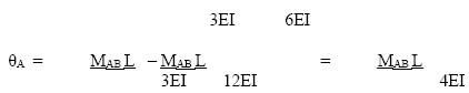
From above, MAB = 4EI θA / L.
If we equate θA to one radian, the value of moment becomes
MAB = 4EI / L
The above expression, which provides the value of moment required at one end to induce unit rotation there, is known as the rotational stiffness of the member. The notation for this is KAB. It may be noted that this expression of rotational stiffness is for the condition when the other end of the member is fixed.
Second Situation: End B is on hinge and is free to rotate
In this situation, when a moment MAB is applied at A, the moment induced at the other end would be zero due to the hinge effect. The rotation at A,

Hence, MAB = 3EI θA / L.
As per the definition of rotational stiffness, the value of θA would be equal to one unit:
KAB = MAB = 3EI / L
Carry-over factor
While deriving the rotational stiffness of a member for the above two situations, we have seen that in the case of end B fixed, the moment induced at B would be half of the moment introduced at A. This means that one half of the moment at A has been carried over to B. This factor of ½ is known as the carry-over factor.
In the case when the end B is hinged, the carry-over factor is zero.
These values of carry-over factors greatly help in making an assessment of the moment values at the other end during process of iteration.
Lateral stiffness of members
Lateral stiffness of the member is the magnitude of moment, which gets induced at the end A of the member AB when a relative displacement of unit magnitude takes place between the ends A and B of the member.
Similar to the conditions for rotational stiffness, the value of lateral stiffness is also dependent on the support condition of the other end.
When the end B is fixed
In the case when both ends of the beam are fixed, the moment at one end is due to relative deflection ‘d’ with the other end:
M = 6EId / L2
The value of lateral stiffness in this case (value of moment when d = 1),
LS = 6EI / L2
When the end B is on hinge and is free to rotate
The value of lateral stiffness in this case would be equal to
LS = 3EI / L2
Distribution factor
In the case of frames or any other structural system, where more than one member joins at a node, that joint is assumed as rigid. It means that even if the joint as a whole rotates due to load application, the individual members still maintain the original slopes between them. This implies that all the members undergo the same amount of rotation.
If a number of members are meeting at a joint which undergoes rotation due to moment application of magnitude M, then this moment shall be shared by each member in proportion to its rotational stiffness with respect to the cumulative value of the rotational stiffness of all members meeting at the joint.
Therefore, if the cumulative value of rotational stiffness at the joint is Kcum and the value for the member under consideration is K’, the moment carried by the member shall be
M’ = (K’ / Kcum) M
This factor K’/Kcum is known as the distribution factor for an individual member.
4.6.2 Application of moment distribution method
The step-wise description of the application of the moment distribution method is as follows:
- First of all, it is required to calculate the fixed end moment for each member under the applied load, in a manner similar to that described in the slope-deflection technique. While doing this, both the ends of the members shall be considered as fixed, irrespective of their actual structural status.
- The next step in the process is to work out the rotational stiffness of members at each joint. The expression K = 4EI/L would be used to determine it. It may be noted here that even if the other end of the member is hinged, it is procedurally correct to use the value of stiffness considering the other end as fixed and then release the fixity of the end in every cycle in the way described under (5). Otherwise, for hinged ends, the expression K = 3EI/L can also be used and it would obviate the need of repeating the release of the joint in each subsequent cycle.
- With the help of the values of individual K’s for each member, the values of the distribution factor for each member converging at the joint would be determined.
- This entire information about the fixed end moment and the distribution factors shall be recorded in a tabular form. The format of the table would be described in the illustration below.
- The further step would involve the releasing of the joints, which are actually hinged but were considered fixed. To do that, a moment, which is equal to the fixed end moment in magnitude, but of opposite sign, shall be applied to the joint.
- Together with this, the joints, which have more than one member meeting, would need balancing of the moment. In the act of balancing, the net moment at the joints, due to the applicable fixed end moments, would be determined first. This would be the algebraic sum of all the moments. Once determined, this unbalanced value of the moment shall be balanced by applying a moment at the joint, equal in magnitude to the unbalanced moment but opposite in direction.
- The distribution of this balancing moment shall be in proportion to the distribution factor of the members meeting at the joint.
- Once the joints have been released/balanced in the way described above, the carry-over of the moments applied would need to be considered. As we have observed in concepts, half of the moment applied at one end of the member gets carried-over to the other end.
- Once the carry-over (CO) cycle is completed, the joints will again turn non-balanced. This would need further cycles of joint releasing/balancing activities, accompanied with the carry-over of the moments.
- After a number of balancing cycles, the carried-over moments would become too small. The procedure would be stopped at that point. The last cycle would consist of the joint balancing operation but no carried over to the junctions. However, carry-over to an end joint can be performed.
- The algebraic sum of the value of original fixed end moment and the subsequent values of all the balancing and carried-over moments for any end (all the moments figuring in single column) shall be the value of the final end moment.
The following illustrations would further clarify the procedure.
Illustration 4.11: The continuous beam ABC has ends A and C supported over a hinge. The point B is continuous over the supports. The spans, load imposed and relative moment of inertia for each member are shown in Figure 4.22. We have to draw the bending moment diagram.
First of all, the fixed end moments for each span would be calculated as follows:

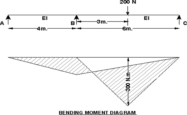
Bending moment diagram – illustration 4.11
Also, the values of rotational stiffness of each member shall be determined by considering both the ends as fixed:
KAB = 4EI/4 = EI,
KBC = 4EI/6 = 0.67 EI
The values of distribution factor for the nods B are as follows:
DBA = EI/ (1+0.67) EI = 0.60
DBC = 0.67EI/ (1+0.67) EI = 0.40
The fixed end moments and the distribution factors have been tabulated as below.
The next step is the release of the joint C from an assumed position of fixity. It may be noted that due to non-imposition of load on span AB, the fixed end moment anyway is equivalent to zero. Thus, there is no need to apply the procedure on joint A.
To achieve release of joint C, moment of magnitude –1500 NM would be applied at C. Half of it would get transferred to the other end (B) of the span.
The next step would be the balancing of the joint B.
At B,
| Unbalance Moment | = − 1500 − 750= | − 2250 |
| Balancing Moment | = 2250 |
The balancing moment at B would be distributed in proportion of the distribution factors:
| Towards A | = | 0.6 X 2250 | = | 1350 |
| Towards C | = | 0.4 X 2250 | = | 900 |
Half of the magnitude of these moments would be carried-over to the other respective ends, A and C.
In the next step, the ends A and C would be released from the carried-over moments by introduction of moments of similar magnitude but
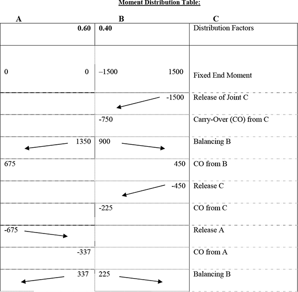
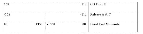
The resultant bending moment diagram is shown in Figure 4.22.
Illustration 4.12: The continuous beam ABCD has ends A fixed and D supported over a hinge. B and C are continuous over the supports. The spans, load imposed and relative moment of inertia for each member are shown in Figure 4.23.
First of all, the fixed end moments for each span would be calculated as follows:
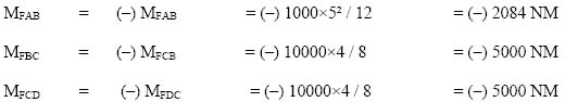
Also, the values of rotational stiffness of each member shall be determined by considering all the ends fixed:
| KAB | = | 4EI/5 = 0.8 EI, |
| KBC | = | 4EI/4 = EI, |
| KCD | = | 4EI/4 = EI |
It should be noted here that the value of KCD has been determined by assuming end D as fixed and, therefore, it would be necessary to release the joint D in each cycle.
The values of distribution factors for the nodes B and C are as follows:
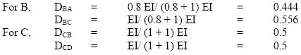
These values of fixed end moments and distribution factors have been joint-wise tabulated on the next page.
The next step is the release of the joint D from an assumed position of fixity. It may be noted that since joint A is fixed originally, there would be no need to release this joint. To release D, the moment of magnitude –5000 NM would be applied.
The next step would be the balancing of the joints B and C.
At B,
| Unbalance Moment | = − 5000 + 2084 | = | − 2916 |
| Balancing Moment | = 2916 |
The balancing moment at B would be distributed in proportion of the distribution factors:
| Towards A | = | 0.444 X 2916 | = | 1295 |
| Towards C | = | 0.556 X 2916 | = | 1621 |

Bending moment diagram – illustration 4.12
Once these two moments are applied at junction B, half of these would carry forward to the other respective ends.
Moment Distribution Table:
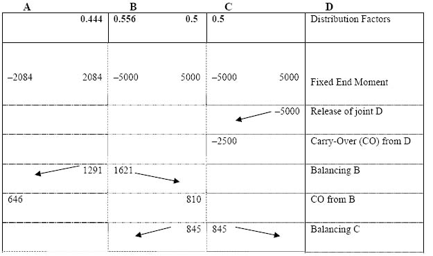
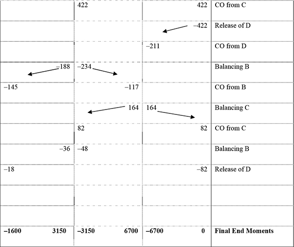
The joint C was originally in a balanced state but after release of joint D and the moment carry-over from B it has turned unbalanced:
| Unbalance Moment | = −2500 + 810 = | −1690 |
| Balancing Moment | = 1690 |
The balancing moment at C would be distributed in proportion to the distribution factors:
| Towards B | = | 0.5 × (1690) | = | 845 |
| Towards D | = | 0.5 × (1690) | = | 845 |
Once these two moments are applied at junction C, half of these would carry forward to the other respective ends.
After this carried over operation, the end D and joint B have again turned unbalanced. Therefore, we need to repeat the cycle of releasing, balancing and carry-over once again for these two.
Again, with the carry-over performed from B and D, the joint C has unbalanced moment. We need to balance the joint C once again. This, along with resultant carry-over, is shown in the table.
In the next step, the balancing of B and D has been done. Since the values of carry-over moments have become quite small now, we have decided to stop the process here itself. The values of end moments have been worked by algebraically summing all the moment values into a single column.
It is noticeable that the algebraic sum of all the moments at mid joints B and C has been zero, which is a conceptually correct situation.
Once the end moment values are derived, the further procedure of drawing the bending moment diagram and shear force diagram is similar to the one adopted in the slope-deflection method.
The resultant bending moment diagram is shown in Figure 4.23.
Illustration 4.13: The frame ABCD has ends A and D supported on a hinge. The nodes B and C are rigid, but unsupported. The spans, load imposed and relative moment of inertia for each member are shown in Figure 4.24.
Both frame and loading are symmetric in this case and, therefore, there would be no-sway in the frame.
First of all, the fixed end moments for each span would be calculated as follows.
| MFAB | = | MFAB | = 0 |
| MFBC | = | (−) MFCB | = (−) 1000×62 / 12 = (−) 3000 NM |
| MFCD | = | MFDC | = 0 |
Next, the values of rotational stiffness of each member shall be determined in accordance with the actual end conditions:
| KAB | = | 3EI/4 | = 0.75EI, (End A is hinged) |
| KBC | = | 4E (2.25I)/6 | = 1.5EI, |
| KCD | = | 3EI/4 | = 0.75EI (End A is hinged) |
The values of distribution factors for the nodes B and C are as follows:
For B, DBA = 0.75 EI/ (0.75 + 1.5) EI = 0.333
DBC = 1.5 EI/ (0.75 + 1.5) EI = 0.667
For C, DCB = 1.5 EI/ (0.75 + 1.5) EI = 0.667
DCD = 0.75 EI/ (0.75 + 1.5) EI = 0.333
These values of fixed end moments and distribution factors have been joint-wise tabulated as described in the previous illustration.
The procedure adopted in moment writing in the table is self-explanatory. The only noticeable point is that there has been no moment carry-over shown toward ends A and D. The reason for this is the hinge supports at both the ends. Due consideration has been given while calculating the rotational stiffness of the members AB and CD. Incidentally, in this case, the values of fixed end moments at A and D are zero, due to the absence of any loads on the spans. Had there been any fixed end moments present for these ends, it would have necessitated the inclusion of a step, for release of these two joints to make their fixed end moment zero.
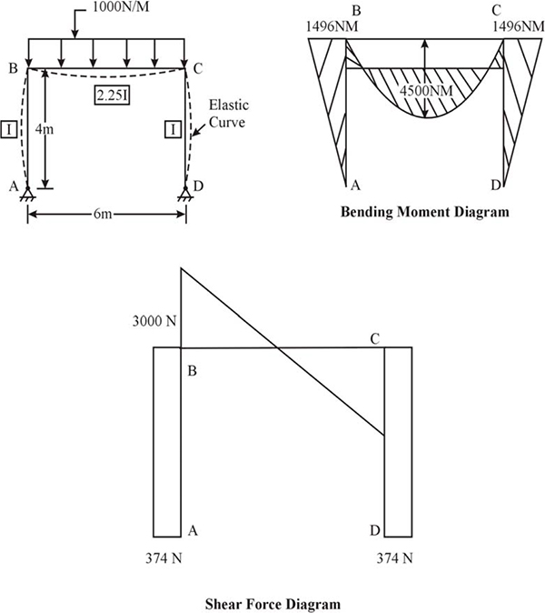
Bending moment and shear force diagrams – illustration 4.13
Moment Distribution Table:
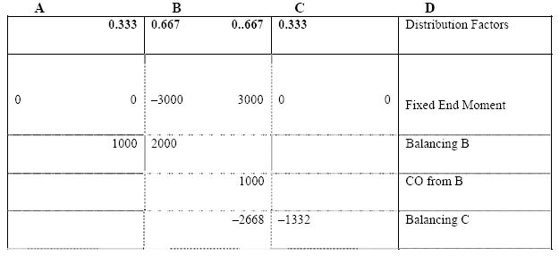
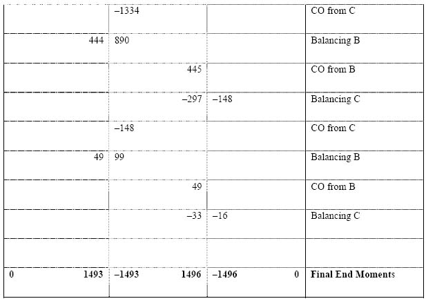
The slight variation observed in the values of the moments at joints B and C is due to the inherent characteristics of the procedure. The accuracy level of the results increases, with the number of cycles performed. We will rationalize the absolute moment values to 1496 NM.
With the fixed end moments known, the bending moment diagram for the frame ABCD is shown in Figure 4.20.
To draw the shear force diagram, the end shear force due to moments has been calculated as follows:
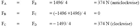
The shear force diagram and the elastic curve for the frame are shown in Figure 4.20.
Analysis of frames subjected to ‘sway’
If the frame is subjected to sway, the analysis by moment distribution method involves preparation of more than one moment, balancing tables. The first table will derive a usual ‘no-sway’ solution, by assuming that the sway is prevented by introduction of some restraint.
The next step would be to assign an arbitrary value of sway d, in the direction consistent with the load arrangement, preferably in terms of some multiple of EI. With the help of a lateral stiffness expression of each member, the end moment values for the joints will be derived exclusively, due to the sway. At this stage, another set of moment distribution shall be performed in order to derive the set of end moments, due to sway.
Since the sway value was assumed arbitrarily, the final step would be to apply the correction factor to the values of end moments due to sway. For this, the net horizontal shear in the first case would be determined. This would necessarily be =/= 0; otherwise, the sway would not have taken place. Suppose the value of this net shear force is V. For the overall stability, the net value of shear in the sway case should have been equal to (–) V. If it is different from (–) V, the factor likely to make it (–) V is called the correction factor.
The ultimate end moment values are the algebraic sum of the end moment due to normal loading and the factored end moment, due to sway.
The following illustration should make the procedure clear.
Illustration 4.14: The frame ABCDEF has ends A and D as fixed supports and F is supported on a hinge. The nodes B and C are rigid, but unsupported. The spans, load imposed and relative moment of inertia for each member are shown in Figure 4.25.

Bending moment diagram and elastic curve – illustration 4.14
In this case the frame itself is symmetric but is subjected to asymmetric loading and, therefore, there would be sway in the frame.
In the first step, the frame would be solved for loads applied, assuming it to be a non-sway case.
Step – I: No-sway solution
First of all, the fixed end moments for each span would be calculated as follows:
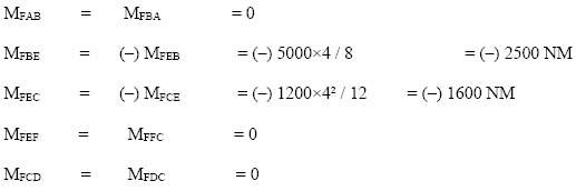
Next, the values of rotational stiffness of each member shall be determined in accordance with the actual end conditions:
| KAB | = | KCD | = | 4EI/5 | = 0.8EI, |
| KBE | = | KED | = | 4E (2I)/4 | = 2EI, |
| KEF | = | 3EI/5 | = 0.6EI (End F is hinged) |
The values of distribution factors for the nodes B and C are as follows:
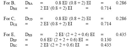
These values of fixed end moments and distribution factors have been joint-wise tabulated as follows.
Moment Distribution Table:
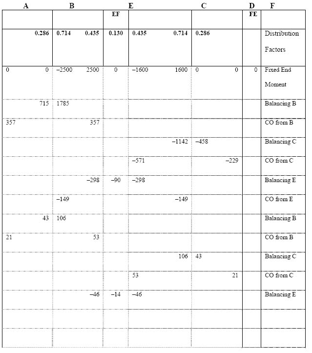
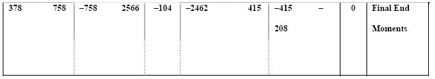
Step – II: Sway solution
For this part, let’s assign an arbitrary value of 2500/EI to the sway d. The direction of sway is assumed such that the members AB, FE and DC rotate clockwise.
In this situation,
MFAB = MFBA = 6EId / L2 = (6EI×2500/EI) / 52 = 600
MFCD = MFDC = 6EId / L2 = (6EI×2500/EI) / 52 = 600
But since the end F is hinged,
MFEF = 3EId / L2 = (3EI×2500/EI) / 52 = 300
And MFFE = 0.
Moment Distribution Table:
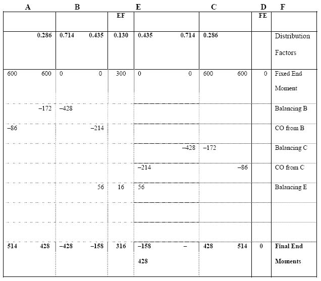
Step – III: Determination of correction – factor
As the values of end moment determined for sway are based on an arbitrarily assumed magnitude of sway, we are required to determine its correction factor.
For this, the value of net horizontal shear force in the ‘no-sway’ condition is
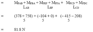
And the value of net horizontal force in the ‘sway’ condition is
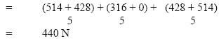
The correction factor k would be determined from the relationship
81.8 + k×440 = 0
Hence, k = (−) 0.186.
With this value of correction factor, the net composite values of end moments are as follows.
| Designation | End Moment : No-sway (A) | End Moment: Sway (B) | Correction Factor X End Moment: Sway (C) | Net End Moment in NM (A + C) |
| MFAB | 378 | 514 | –96 | 282 |
| MFBA | 758 | 428 | –80 | 678 |
| MFBE | –758 | –428 | 80 | –678 |
| MFEB | 2566 | –158 | 29 | 2595 |
| MFEF | –104 | 316 | –59 | –163 |
| MFFE | 0 | 0 | 0 | 0 |
| MFEC | –2462 | –158 | 29 | –2433 |
| MFCE | 415 | –428 | 80 | 495 |
| MFCD | –415 | 428 | –80 | –495 |
| MFDC | –208 | 514 | –96 | –304 |
The bending moment diagram and the elastic curve (deflected shape) of the structure are shown in Figure 4.21. The procedure to draw the shear force diagram is standard for this situation, too.
After understanding both slope-deflection and moment distribution techniques, we can appreciate the obvious simplicity of the moment distribution technique. The technique obviates the need to write equations for each fixed end moment, as well as the solution of a set of simultaneous conditional equations, which emerge from these end moment equations. Although the results derived from moment distribution techniques are not hundred percent accurate, it is possible to reach to a very high degree of accuracy by increasing the number of iteration cycles. For most of the problem though, an acceptable degree of accuracy is reached after just one or two such cycles.
4.7 Influence line diagram for statically indeterminate structures
We have studied the concept and usefulness of influence lines in Section 2.11. In that section, we have seen how the influence line can be useful for determination of various stress functions, in the case of statically determinate structures. In this section, we will study the technique of drawing influence lines for statically indeterminate structures and their use in analyzing such structures.
To reiterate, the influence line is a graphical representation of the magnitude of a reaction or stress function on a section of the span, when a unit concentrated load moves along the span. The influence line can be quite helpful for the situation, when the load system on the structure is not stationary. Therefore, this fact needs consideration in the analysis.
In the case of statically determinate structures, the analytical method of drawing an influence line diagram is quite simple, as we have seen earlier. It is based on the principles of statics. In the case of statically determinate structures, the procedure of drawing an influence line diagram for a stress function is obviously not that simple. There are a number of techniques to draw influence lines. A good example is the application of ‘the principle of virtual work’. The most widely used method for this category of structures is the application of the ‘Muller–Breslau’s principle’, which can be backed by any other quantitative technique such as moment distribution to determine the ordinates.
4.7.1 Muller–Breslau’s principle
Muller-Breslau’s principle states:
For any structure, if a unit deformation, consistent with a stress function, is introduced at a section, keeping other restraints unchanged, the resultant deflected shape of the structure in its inverted form will represent the influence line at the section, for that particular stress function on some scale.
To fully understand this statement, some clarifications will definitely help.
First of all, it would help to explain the phrase a unit deformation consistent with a stress function. The stress functions are the functions like bending moment, shear force, deflection, etc. The deformations consistent with each of these would have taken place, had there been no resistance offered to those stress functions at that section. For instance, for bending moment it is the slope at that section. Introduction of a hinge eliminates the moment-carrying capacity of the section. Also, the slope at the hinge should assume a unit value (one radian). This aspect has further been treated in detail in the following paragraphs.
The expression inverted form means that the deflected shape is rotated about the base line. We have adopted the sign convention for stress functions like bending moment, shear force, etc. In the graphical representation of these stress functions, for a particular structural condition, the ordinates above the base line indicate positive values and ordinates below the base line indicate negative values of the stress function. The condition of inverted form implies that the ordinates above the base line, for deflected shape would indicate negative values and the ordinates below it would indicate the positive values in the case of influence line.
The other important thing to observe is the use of the expression at some scale. When we introduce a unit value of the deformation at the section, we can, with reasonable accuracy, draw the deformed shape of the structure, consistent with the support conditions. In the case of a simple statically determinate structure, it is possible to determine the ordinates of the influence line at different sections. In the case of statically indeterminate structures, however, it is not possible to just measure the ordinates in the deformed shape to get their values at different sections along the span of the structure. Therefore, the procedure of drawing influence lines by use of Muller–Breslau’s principle is a qualitative one. It can provide good information on the nature of the stress functions, generated by the shifting location of loads, but at the same time cannot directly provide the absolute values. At certain times, it may be enough to have this qualitative information alone to take decisions about structural arrangements. There are times, however, when it is imperative to know the ordinates. A separate quantitative analysis would be needed at such times.
4.7.2 Influence line using Muller–Breslau’s principle
We have understood the principle in the previous section. Here, we would observe the application of the principle to draw the influence line diagram for different stress functions.
Influence line for bending moment
We consider the case of the statically indeterminate beam ABCD, with both the supports on hinges and the beam continuous over both the mid supports. A unit load is moving along the span and has presently occupied a position in the span CD. Due to its present location, the elastic curve for the beam has adopted the shape shown in Figure 4.26. Although this step is not essential, it provides the idea about the shape the elastic curve would take under restraints imposed.

Influence line for bending moment
Influence line for shear force
We will again consider the case of the statically indeterminate beam ABCD of the previous sub-section.

Influence line for shear force
To draw the influence line diagram for shear force, we again select the same section I-I on span BC. The next step has been to introduce a cut at the section and apply a force in such a way that results in a unit relative displacement, between the points on either side of the cut. At the same time, the slopes on either side of the cut would be similar. The deformed shape of the beam in this situation is shown in the same diagram. Since the reverse of it would be the influence line at some scale, the shape of the influence line is shown in Figure 4.27.
Influence line for support reaction
For this too, we consider the case of the statically indeterminate beam ABCD of the previous sub-section.
To draw the influence line diagram for support reaction, we select the support C. The next step is to remove the constraint of ‘no-settlement’ at C and apply a force in such a way that results in a unit magnitude of settlement at C. The deformed shape of the beam in this situation is shown in the same diagram. Since the reverse of it would be the influence line at some scale, the shape of the influence line is shown in Figure 4.28.

Influence line for support reaction
Influence line for support moment
For support moment, we need to consider one of the internal supports only, since for end supports the moment would always remain zero. For this too, we consider the case of the statically indeterminate beam ABCD as in the earlier examples.
To draw the influence line diagram for support moment, we select the support C. The next step is to insert a ‘hinge’ at C and apply a force in such a way that results in a unit angle of rotation at C. The deformed shape of the beam in this situation is shown in the same diagram. Since the reverse of it would be the influence line at some scale, the shape of the influence line is shown in Figure 4.29.

Influence line for support moment
4.8 Conclusion
In this chapter, we have studied the techniques dedicated to the analysis of the continuous beams, as they are one of the most commonly encountered statically indeterminable systems. We can now also analyze other beam systems such as fixed beams, propped cantilevers, etc.
We have also studied the analysis techniques, which are useful for the analysis of frames and other structures, in addition to beams. For this, the techniques of slope-deflection and moment distribution were described. These are the two most commonly used techniques for this purpose. With these two known, it is possible to analyze almost any kind of structural arrangement with ease.
We ended the section on the introduction by explaining the method of drawing influence line diagrams for statically determinate structures. We have already studied influence lines and their use in the case of statically determinate sections in Chapter 2. The information on the Muller–Breslau principle supplements the earlier material studied on influence lines.
In the previous three chapters we have observed the analysis of statically determinate and indeterminate structures separately, as well as studied the principles and applications of the strength of materials. With this, we are ready to move to practical applications of these principles, for actual design exercises. We will study the types of loading, failure mechanisms and major design theories in the next chapter.
This chapter will help the reader to understand situations which lead to the failure of engineering materials and, consequently, the structures. The chapter further describes design theories, which accommodate material behavior.
Learning objectives
After completion of this chapter, one will be able to:
- Understand the physical characteristics of commonly used structural materials
- Understand the failure mechanism of such materials under different stress conditions
- Fully appreciate the different design theories which are applied in practical design
- Understand the process to capture the worst effect of combined load application during structural analysis
In the previous chapters, we have studied and understood the types of structures and the nature of response they offer to external force application. We have also studied the physical properties of the materials of construction, which determine the magnitude of deformation under stress. We also need to understand the failure condition of a material and the mechanism of failure. Once that is understood, it would be easy to appreciate design theories and the inbuilt safety factors.
5.1 Stress–strain relationship for different materials
While analyzing a structure so far, we have throughout treated Hooke’s law as valid. The law states that ‘within elastic limits, the stress is directly proportional to strain’. The reason we treated this valid is that for the structural elements, we have so far decided to treat the deformations within elastic limits only. Plastic deformations, which are permanent in nature, are not permitted to occur in the engineering structures for obvious reasons. The condition of proportionality of stress and strain makes it simple to derive a number of relationships.
Experiments have shown that a large number of materials obey Hooke’s law, as long as they are stressed within a limit. This limiting value of the stress varies for different materials. Once the stress crosses that limit, the materials start exhibiting some non-linearity between stress and strain. The materials, however, still retain elastic properties and regain the original shape on removal of loads. The limit up to which stress and strain remain proportional to each other is known as the proportionate limit for the material.
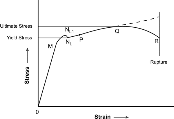
Stress–strain diagram for mild steel
It is interesting to observe the stress–strain behavior of the material, beyond this proportionate limit. The standard tensile stress test, performed on a specimen of the material, would be a guide for it. The modulus of elasticity (E) of the material does no longer govern the relationship in this zone. The typical shape of the stress–strain diagram, in the case of low carbon steel (mild steel), is shown in Figure 5.1. The portion OM of the curve indicates the linear relationship between stress and strain. The modulus of elasticity (E) represents the slope of the curve in this portion. Beyond point M, the slope of the curve becomes steeper as the magnitude of strain increases at a much higher rate in this zone. This portion has been shown as MN in the curve. The material retains its elastic properties till N, which represents the limit of elasticity. At N, the material becomes plastic and the magnitude of strain increases without any appreciable increase in the stress. This phenomenon is known as the ‘yielding’ of the material. Accordingly, the point N is known as the yield point of the curve.
Here, it is important to mention a feature which is often observed while drawing the curve. The value of the stress actually tends to show a sudden drop, after reaching a point and the yielding actually begins, from this lower point. The point on the crest is known as the upper yield point and the one in the valley is known as the lower yield point. In the diagram, they have been designated as NL1 and NL respectively.
The reason of the generation of multiple yield points is actually machine’s inertia. The plastic stretching begins suddenly and this results in a sudden drop in the stress at that instant. The yielding begins actually at NL and NL1 is some sort of false yield point. In cases where both upper and lower yield points are visible in the curve, it is the lower yield point value, which is adopted for structural engineering purposes. There can also be cases when more than one set of upper and lower yield points are visible in the graph. In such cases, the stress value represented by the final lower yield point is adopted. The stress corresponding to yield point is known as the yield stress for the material.
Coming back to the curve of the diagram as shown in Figure 5.1, the portion NL to P represents yielding of the steel material. This is the plastic deformation phase of the material. Beyond P, the material recovers some of the elasticity and starts offering resistance to strain. From here, the further strain is accompanied with a somewhat appreciable increase in the stress. The stress–strain curve moves upwards till point Q, after which the value of strain starts declining. This apparent decline, in the stress, is the result of the reduction of the cross section of the specimen. This reduction becomes quite appreciable at this stage and can even be noticed by a mere viewing. As per convention, the value of stress in the specimen is calculated, without giving any consideration to this reduction in area. Therefore, despite the increase in the actual stress level, it seems that the magnitude of stress has declined in this phase. This phase continues up to point R where the fracture of the specimen takes place.

Stress–strain diagram for cast iron
As there has been a convention to calculate the value of stress based on original cross section of the specimen, the value of stress at Q becomes the largest. This value is known as the ultimate stress for the material.
Mild carbon steel is one of the few materials (and perhaps the only structural material), which exhibits a prominent yield point under conditions of stress. Other structural materials show a gradual transition, from the linear or proportional range to the nonlinear range of stress–strain relationship. To illustrate the behavior of brittle materials under tensile stress, the stress–strain diagram for cast iron is shown in Figure 5.2. As is obvious, the material crosses the proportionate limit at quite a low value of stress. It also exhibits no marked yield point.
It is possible to obtain the stress–strain diagrams for axial compression too, by performing a direct compression test on a specimen of the material. These graphical presentations of stress–strain relationships are very useful to help determine the values of characteristic stresses such as the proportional limit, yield point, ultimate stress, etc. These characteristic values of structural steel are largely similar in the case of compression and tension.
5.1.1 Behavior of steel beyond the yield point
When a mild steel specimen is stretched beyond its yield point, the material hardens and the value of stress imposition as value of stress imposition goes up the bar elongates. At this stage, elongation of the specimen is accompanied with uniform reduction of the cross-sectional area so that overall volume of the specimen remains practically unchanged. The major part of the mechanical energy given at this stage is converted into heat, while a smaller part of it remains in the specimen in the form of strain energy.
Types of tension fractures
In a material, one of two types of fractures can be observed: brittle fracture or shear fracture as in the case of mild steel, aluminum and other metals. In brittle fracture, which is the case with cast iron, fracture occurs over the entire cross section, practically without any plastic deformation of the specimen. In the shear fracture, which is observed in materials like mild carbon steel and aluminum, fracture occurs after considerable plastic deformation. It normally leaves one part of the fractured specimen with a projection and the other with depression or socket. The explanation is that if for the given material the resistance to sliding is greater than the resistance to overcome the cohesive force between the grains, the result would be a brittle failure. The reverse would be true for the shear failure of the material.
5.2 Design philosophies
Two major philosophies exist, which are used to design structures with adequate strength. These are as follows.
- Working Stress Theory: According to this theory, the design ensures that the value of stress in any component of the structure does not exceed the failure value or perceived failure value, divided by a factor termed as factor of safety.
- Limit Design Theory: According to this theory, the components of the structure are designed to withstand a particular value of load, which is determined by multiplying the magnitude of service loads with a factor. This factor is termed the load factor. The value of the load factor is dependent on the nature of the load.
5.2.1 Working stress theory
In the elastic design process, the requirement is to simultaneously fulfill the equilibrium condition, the compatibility condition and the limiting stress condition. According to the first condition, the structure subjected to loading should remain in equilibrium. According to the second condition, the deformation of the various fibres should be compatible with those of the adjacent fibres. According to the third condition, the maximum stress at any section in any fibre should be less than the yield stresses; in other words, the bending moment at the section should be less than the yielding moment.
A stress–strain diagram gives valuable information on the mechanical properties of a structural material. With information on the limit of proportionality, yield point stress and the ultimate failure stress of the material, it is possible to establish the magnitude of stress, specific to any engineering use, which may be considered a safe stress. This stress is typically known as the working stress, and is applied as a limiting value for design of the structural members in the ‘working stress method’ of design.
As a principle, working stress is determined by the following relationship:
Working Stress = Failure Stress / Factor of Safety
Different factors govern the selection of the basis for working stress, for different materials. For instance, in choosing the magnitude of the working stress for steel, it is taken into consideration that, at stress level below the yield point, the material may be considered as perfectly elastic. Beyond this limit, a part of the strain usually remains after unloading the structure, which results in permanent deformation or set. In order to ensure that the structural components remain in the elastic condition throughout, as well as to eliminate the possibility of a permanent set in the components, it is sensible to keep the working stress within the yield point limit. As the yield point stress is quite easy to determine with the help of the stress–strain curve, the working stress value can easily be correlated to the yield point for structural steel.
In the case of materials like concrete, the value of crushing strength of the specimen is the most important, since concrete is essentially designed to withstand compression. For other brittle materials such as cast iron, various kinds of stone and also for such material as wood, the ultimate strength is usually taken as a basis for determining the working stresses.
Factor of safety
The factor of safety is the number by which the failure stress of the material is divided to determine the value of working stress (also, permissible stress) for the material. The historical value of factor of safety used to be high, resulting into small value of working stress. Due to advanced research in recent years and the experience gained in structural engineering, the value of the factor of safety has been rationalized. Consequently, the factor of safety adopted nowadays is comparatively small. This does result in an appreciable savings in material.
The main reasons for not allowing failure stress to reach into a structure and the factors affecting the value of factor of safety are as follows:
- The exact assessment of the value of failure stress is very difficult. The average strength of materials is determined after testing a number of specimens. The strength of different specimens of given structural materials is not identical and some of the specimens may show relatively large deviations in strength, from the average.
- The determination of the magnitude of actual loads on structures is quite complex. The values of dead loads can of course be determined accurately. Live loads, impact loads, wind loads, snow loads, etc., cannot be determined with similar accuracy since these are estimated with the help of statistical data. The values of such loads are therefore only probable but never certain.
- The method to analyze and assess the internal forces in structures has several assumptions built-in, all of which may not be valid in all conditions. The degree of precision varies for different methods. If the method of structural analysis is detailed and precise, it is possible to adopt a small value of factor of safety.
- In addition to known loads, structural elements are sometimes subjected to uncertain stresses such as during erection/fabrication, etc. For instance, the operation of welding may result in high residual stress in a steel structural member. Some safety provision in design becomes necessary to take care of such stresses.
- Factors such as variation in temperature, quality of workmanship, settlement of supports, etc., are also difficult to quantify. Many times, a well-designed structure can fail because of these effects. As a result of corrosion, the overall load carrying capacity of material also decreases during its life span.
- Types of load applications also influence the selection of value of factor of safety. A comparatively small factor of safety (say, 1.5) will give a liberal value for the working stress, provided that only constant loads are acting upon the structure. In the cases of suddenly applied loads or variable loads (and these occur very often in machine parts), larger factors of safety may be necessary.
- The failure of some small structures or some elements of a structure can be less disastrous than the failure of large structures or a major element of a structure. This factor also has a bearing on finalizing the value of factor of safety.
5.2.2 Estimation of ‘Factor of Safety’
It would be worthwhile to develop a mathematical model, which can help in determining the factor of safety, for a given condition. Such relationships for the factor of safety may be decided by defining it in a rational method. As is obvious, the factor of safety may be defined as the ratio of computed strength, T, of the structure or the structural element to the respective computed internal force, F.
Therefore,
Factor of Safety M = T / F
The magnitude of lowest probable strength, T, is influenced by the uncertainties in the mechanism failure, properties of material and the workmanship. The magnitude of highest probable internal load, F, is influenced by the uncertainties in loading conditions, structural behavior, method of analysis, etc. These uncertainties make the probable values of T and F deviate from the computed values.
The minimum probable value of strength is expressed as follows:
Tmin = (T – ΔT)
where ΔT = maximum probable deviation of actual value from the computed value of strength.
Similarly, the maximum probable value of the internal force is expressed as follows:
Fmin = (F + ΔF)
where ΔF = maximum probable deviation of actual value from the computed value of internal load.
We now will define the limiting condition to prevent structural failure. If the minimum probable value of strength is just equal to the maximum probable value of the internal load, then the failure of a structure is just prevented under most severe conditions.
Expressed mathematically, it would be
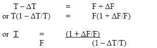
As we have seen earlier, T/F = M, the factor of safety.
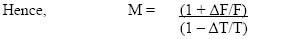
With this, we can now determine the value of factor of safety. In the above expressions, the values of subexpressions ΔF/F and ΔT/T can be assigned values as percentages, depending on the assessment of the situation.
Again as a limiting case, let us assume that the values of deviations ΔF and ΔT in terms of percentage are 25% of the respective calculated values. In that case,

or M = 1.25 / 0.75 = 1.67
This value of 1.67 for factor of safety, though just indicative, can be considered as its minimum value.
It may be understood here that in the case of a statically determinate structural system, the stresses in the structural components will vary in proportion to the applied loads, even if the proportionate limit is exceeded. Thus, in such systems, the application of the working stress method fulfills the desired objective. However, in the case of a statically indeterminate structural system, the stresses in the members are the functions of their deformations. Here, the methods of analysis based on Hooke’s law do not apply beyond the proportionate limit.
5.2.3 Limit-state theory
The previously described working stress design procedure incorporates a single all-embracing safety factor. This safety factor would be appropriate for some aspects of the design, but may not necessarily be appropriate for all. This can lead to inefficiencies in design or even an unacceptable risk level.
Limit state is a way of designing an object by separately ensuring that it can perform each of the required functions. The method takes account of the risk involved, the factors that affect the object’s ability and the factors that affect the anticipated duty or loading. Limit-state design of structure enables one to predict loading, under which the structure will collapse due to simultaneous failure of some or all of its members. According to this theory, we multiply the actual service load with a load factor n and undertake the design treating this inflated load as the collapse load. This way, a true factor of safety n is realized against complete failure of the structure. This is the philosophy of limit design, which is gaining increasing favor among design engineers because its application normally results in more efficient and economical designs.
Serviceability and strength are the two limit states used in the design of structures. Limit state of serviceability is the level at which the structure remains fully functional, with no permanent distortion of the components and also keeping the magnitude of deflection within an acceptable limit. Strength limit state is the point beyond which the structure would no longer stay in place or no longer sustain the imposed loads.

Idealized stress–strain diagram for mild steel
To start with, it is convenient to represent the portion within curve OYMN of the stress–strain diagram for steel, as shown in Figure 5.3. The assumption made here is that the yield point is the limit of proportionality and the material deforms indefinitely beyond it. Therefore, the material is said to be either perfectly elastic or perfectly plastic, depending on whether the stress is below or above the yield point value. It will be further assumed here that the yield point has the same values in both tension and compression. The value of yield stress (fy) for ordinary structural steel may be taken as 280 Newton/mm2.
The strength of steel is expressed in terms of its yield stress. The strength of materials, which do not have a distinct yield point, is specified in terms of 0.2% proof stress. This indicates a stress level, at which a residual strain of 0.2% is left over after unloading. High tensile steel, aluminum, etc., fall in this category.
In order to explain the principle of the limit-state design, let us consider the statically indeterminate system, consisting of three members, as shown in Figure 5.4.

Statically indeterminate system
We assume here that all three members are made of similar steel and have the same cross-sectional area (say, A). As is clear, all the members of the system are subjected to direct stresses only. Consider the situation when the magnitude of the load F keeps on increasing. As the magnitude of the load F increases, the values of the axial forces P and Q in the members also increase, but the ratio of P and Q would remain constant during this phase. This situation remains until the load reaches a certain value Pi, at which point, the force in the vertical bar attains the magnitude Fi = fy×A, i.e., the stress in this bar reaches the yield point. At this moment, the material of the vertical member becomes plastic. On further increase in the load F, the vertical member would stretch without further increase in tensile stress within it. In other words, the member will not contribute towards sharing of the incremental load but the inclined bars, subjected to the smaller value of stress would still be elastic and capable of carrying further load. Therefore, as the load F increases beyond the value Fi, the tensile force P in the vertical bar remains constant but the tensile forces Q in the inclined bars continue to increase. At this stage, the earlier relationship describing the ratio of P and Q would not be valid. The only condition now would be to satisfy the equilibrium equation
F = P + 2Q cosθ
On further increase in the load F, finally, the force in the inclined members would also reach the yield point. At this stage,
P = Q = fy×A
Putting these values in the equilibrium equation gives
Fultimate = fy×A (1 + 2 cosθ)
This value of Fultimate is termed as the collapse load or limit load of the structure. A working load F = Fultimate /N will have a true factor of safety N against complete collapse of the entire structural system.
If we evaluate working load as per limit state of strength vis-à-vis the similar value permitted as per working stress principle, for same value of factor of safety, the value permitted by limit state would be higher than the working stress. The reason is that in the case of working stress, no plastic deformations are permitted and the analysis would have restricted the load to the value, which induces yield stress in the vertical member. Therefore, the limit-state design offers a more efficient solution in structural design.
The design principles and their application under limit-state design method have further been elaborated in Chapter 8.
5.3 Combination of loads
It is quite common for the structure to subject to a variety of loads, for instance, dead loads, live loads, nature subjected loads, etc. It is crucial for a well-designed structure that it should be capable of sustaining the most adverse combination of dead loads, prescribed live loads, wind loads, earthquake loads and any other forces or loads to which the structure may reasonably be subjected, without exceeding the stresses specified in the standard. At the same time, the designer is required to be careful to not overestimate the effect of loads, as it may result into a less than efficient design, which can prove uneconomical.
The combined effects of various loads on a structure have been studied extensively and various design codes specify the norms to consider their effects. In principle, the load combinations for design purposes would be one that produces maximum forces and effects and, consequently, maximum stresses. For this, it is considered that all the nature-induced loads would not act together, at a time, over the structure.
Keeping that in consideration, the worst of the following combinations is adopted for the design, both in working stress and limit design processes:
- Dead load + live loads,
- Dead load + live loads + wind or earthquake loads, and
- Dead load + wind load or earthquake loads.
Also, in view of the transient nature of some of these loads, the design codes allow an increase in the permissible stresses if such transient loads are part of the combination acting on the structure. A few of such provisions are described below.
- For rivets, bolts and tension rods, the permissible stresses are increased by 25 percent when the effect of wind or seismic load is taken into account.
- When the effect of wind or seismic load is taken into account, the permissible stresses in steel are increased by 33.33 percent.
For all such situations, the increased values of permissible stresses must not exceed the yield stress of the material.
5.4 Theories of failure
In the case of materials obeying Hooke’s law, there exist definite values of direct stress (σ 0), strain (Є = σ 0 /E), maximum shear stress (σ 0 /2) and total strain energy (σ 02 /2E) at the elastic limit.
The failure of a structure may occur in any one of the following situations. There are various theories that explain the phenomenon of the failure of a structure.
- Maximum Principal Stress Theory (Rankine’s Theory) – According to this theory, failure will occur if the maximum principal stress exceeds the value of direst stress (σ 0 ) at the elastic limit.
For a safe structure,

- Maximum Strain Theory (St. Vanant’s Theory) – According to this theory, failure will occur if the maximum strain exceeds the strain caused by the direct stress at elastic limit.
For a safe structure,
σ 0 ≥ σ 1 – (σ 1 + σ 3 )/m
Maximum Shear Stress Theory (Guest’s Theory) – According to this theory, failure will occur if the maximum shear stress exceeds the shear stress caused by the direct stress at elastic limit.
For a safe structure,

- Total Strain Energy Theory (Haig’s Theory) – According to this theory, failure will occur if the maximum strain energy exceeds the strain energy caused by the direct stress at elastic limit.
For a safe structure,

5.5 Conclusion
In this chapter, we have studied the behavior of common structural material under stress. We have understood the limits of elastic and plastic deformations in the members. We have also understood the importance of this differentiation, which forms the basis of the design theories, as their ways of defining the failure are different.
We have also seen the explanation of two important design theories: working stress and limit state. We are now familiar with the principles and approaches of each. The understanding of these theories is critical, as one needs to understand what is expected as an outcome if one or the other is adopted for the design. We also studied various theories regarding the failures of structures.
All of this knowledge will be used for the study of the actual design of structures in the following chapters of the manual.
This chapter will enable the reader to understand the behavior of steel as a structural material and learn to design various kinds of structures with it, using the earlier understood principles of analysis and design.
Learning objectives
After completion of this chapter, one will be able to:
- Fully understand the behavior of steel as a structural material
- Understand design techniques for various fastening systems in steel structures
- Understand design techniques that use steel in a number of common structures
Steel is one of the most widely used construction materials. The various properties of steel, such as its strength, ductility, and hardness, have attracted the attention of designers for a long time and made it the most widely used metal in construction. Coupled with these properties is the technical advancement made in its manufacturing. It is nowadays very easy to obtain steel with a variety of desired mechanical properties. It is equally easy to source the skills required to convert raw steels into useful structural members. This is done by the use of various fabrication and erection techniques. These factors are responsible for the growing uses of steel for construction.
6.1 Design of structures
We begin by elaborating on the process flow involved in structural design. As discussed earlier, structural design is the process of:
- Selection and finalization of construction materials
- Determination of proper sizes of components, based on the properties of materials and the magnitude of loading
- Finalizing shape of the member components, based on practical considerations
- Designing features such as connections, fastenings, etc.
The selection of construction materials depends upon factors such as availability, economy, compatibility, speed and ease of construction, physical environment, etc. As is obvious, each of the above factors has the potential to influence the final choice of material.
The proper size of a component depends upon the physical properties of the material used, such as ultimate/allowable stress, modulus of elasticity, etc. The consideration is that the stress generation and deformations obtained due to load application should remain within the allowable limits.
Once the sectional properties are determined, the final shape of the components can also be influenced. Certain standard manufactured sizes of components are available. Occasionally, architectural requirements do not allow variation in sizes for different structural components.
After all the component sizes are decided upon, the final step in design process is to provide details of the connections and fastenings. In the case of steel structures, where the construction is not monolithic, details such as method of connection (welding, bolting and riveting) and their sizes are of major importance. In the case of concrete structures, features like treatment of reinforcement steel at critical locations are of prime importance.
It is very important to apply safety checks once the design is completed. It is necessary to verify that the design is up to the standards and has been approved by the concerned authorities.
Once all of these details are worked out, the designer presents all the outputs in the form of detailed working drawings. These drawings clearly show the layout of the overall structure, arrangement of the components, sizes of these components and details of features like connections.
These drawings are generally accompanied with the specifications of work. These specifications describe the materials to be used, testing procedures and acceptance criteria, methodology to be adopted for the construction, its sequence and the necessary precautions to be taken during construction.
6.2 Use of steel for structures
Steel is one of the most widely used construction materials. Concrete and steel together are used for the construction of a vast majority of structures. Steel is quite a versatile construction material. Its use has several advantages; some of them are described below:
- Being factory manufactured, steel can be considered to have a reliable quality and homogeneous characteristics.
- Both compressive and tensile stress-carrying capacity are high in the case of steel, especially when compared with alternatives such as concrete, and therefore designs result into slender and lightweight members.
- It is simpler in the case of steel to design and execute the connections between members and therefore the components can be fabricated in manageable sizes for ease of handling and transportation.
- The speed of construction, when using steel, can be relatively high.
- The individual components of the structure can easily be disbanded and replaced in the case of steel.
The drawback of steel is its limited weather-resistant properties and its susceptibility to corrosion. The cost of construction is usually higher with steel on most occasions. Sometimes, steel is not preferred for aesthetic reasons during construction.
Steel is used for the construction of practically anything, for instance, buildings, sheds, bridges, factories, towers, chimneys, etc.

Bridge made of steel
The photographs of a bridge and an electrical transmission tower are shown in Figures 6.1 and 6.2, respectively.

Transmission tower made of structural steel
6.3 Properties of structural steel
Steel is an alloy of iron. The other ingredients are carbon, sulphur, phosphorus, silicon, copper, manganese, etc. in different proportions for different grades of steel. The steel used for structural purposes is rolled in different flat and long shapes like plates, rolled sections, tubes, etc.
6.3.1 Chemical composition
On the basis of chemical composition, structural steel is generally classified as mild steel, high-carbon steel and low-alloy steel. This classification depends upon the content of carbon and other elements in the steel. Steel of other classifications, i.e., high-alloy steel, is normally used for special purposes and not so much for the manufacturing of structures.
The range of constituents for different classifications of structural steels is as follows:
Mild steel
| Constituent | Carbon | Sulphur | Phosphorous |
| Percentage Range | 0.20 – 0.25 | 0.05 – 0.06 | 0.05 – 0.06 |
High-carbon steel
| Constituent | Carbon | Sulphur | Phosphorous |
| Percentage Range | 0.22 – 0.28 | 0.05 – 0.06 | 0.05 – 0.06 |
Low-alloy steel
Low-alloy steel contains a larger number of elements in comparison with carbon steels. There are different grades of low-alloy structural steel, with varying physical and chemical properties. A sample composition for low-alloy steel is given below.
| Constituent | Carbon | Sulphur | Phosphorous | Manganese |
| Percentage Range | 0.20 – 0.25 | 0.04 – 0.55 | 0.04 – 0.55 | 1.3 – 1.6 |
6.3.2 Physical properties
The physical properties, the magnitude of which can be considered similar to all grades of steels, are as follows:
| Unit Weight | 78.5 kN/m³ |
| Modulus of Elasticity (E) | 2.1 × 10⁵ N/mm2 |
| Coefficient of Thermal Expansion | 12 × 10–6 / ºC |
Apart from these, other important physical characteristics for structural steel are strength, ductility and hardness. The magnitudes of all these characteristics vary, from one type of steel to the other. Out of these, strength is the most important characteristic. It determines the actual section of the structural element. Ductility is important from the point of view of the allowable deformation and is measured as the percentage elongation of the tensile test specimen for steel at the moment of rupture.
The engineering codes of different countries classify structural steel in different grades. The indicative range of yield strength and ultimate tensile strength for different grades of steel is given below.
| General Classification of Steel | Range for Yield Strength in N/mm2 | Range for Ultimate Tensile Strength in N/mm2 |
| Mild-Carbon Steel | 225–265 | 400–540 |
| High-Carbon Steel | 280–360 | 475–600 |
| Medium Strength Low-Alloy Steel | 280–320 | 440–575 |
| High Strength Low-Alloy Steel | 370–530 | 540–800 |
The classifications indicated above are arbitrary and for the purpose of providing an indication of the stress range for steel. However, during actual design process, it is absolutely vital to use the permissible stress values provided by the manufacturer or the relevant code.
6.4 Steel structural sections
As stated earlier, the steel used for structural purposes is the steel rolled in rolling mills. The rolling produces different shapes and forms. Depending on the sectional characteristics, a particular section is selected for the structural situation. The description of some of the commonly used sections is as follows.
Description of some of the commonly used sections
| a. | Plate and Flat Sections | These have an even thickness and are mainly used for manufacturing of built-up sections of desired properties. |
| b. | Beam (I) Section | This is a section similar to letter ‘I’. It is widely used as beams and column sections. |
| c. | Channel (C) Sections | This section is similar to letter ‘C’. It is used mostly as beam, runner, purlin, etc. |
| d. | Angle Section | This two–legged section has both legs perpendicular to each other, forming the shape of a right angle. This type of section has wide applications, as a lean truss member, tension member, built up sections, etc. |
| e. | T-Section | This again is a two-legged section similar to letter ‘T’. |
| f. | Tube Section | This is a thin-walled closed section, normally circular (sometime square or rectangular too). It can be used for frames, trusses, compression members, etc. |
In addition, being a factory-manufactured material, steel members can be manufactured in any shape and size as per the design requirements.
The cross-sectional details of different structural sections are shown in Figure 6.3.

Cross sections of structural sections
6.5 Design of steel structures
As is well understood by now, components of a steel structure should be capable of sustaining the most adverse combinations of dead loads, the prescribed superimposed roof and floor loads, wind loads, seismic forces where applicable, and any other forces or loads to which the building may be reasonably subjected, without exceeding the permissible stresses.
The following methods may be employed for the design of steel structures:
- Simple design,
- Semi-rigid design,
- Fully rigid designs, and
- Plastic design.
Simple design
This method is based on the elastic theory and applies to structures, in which the end connections between members are such that they will not develop restraint moments, affecting the members and the structures as a whole and in consequence the structure may, for the purpose of design, be assumed to be pin jointed. The method of simple design involves the following assumptions.
- The stress–strain relationship for steel is linear.
- The plane sections normal to the axis do remain plane after bending.
- All the beams are simply supported.
- All connections of beams, girders, or trusses are flexible and are proportioned for the reaction shears applied at the appropriate eccentricity.
- The members in compression are subjected to forces applied at the appropriate eccentricities.
- The members in tension are subjected to longitudinal forces applied over the net area of the section.
Semi-rigid design
This method as compared with the simple design method permits a reduction in the maximum bending moment in beams suitably connected to their supports, so as to provide a degree of direction fixity. In the case of triangulated frames, it permits rotation account being taken of the rigidity of the connections and the moment of interaction of members. In cases where this method of design is employed, it is ensured that the assumed partial fixity is available and calculations based on general or particular experimental evidence shall be made to show that the stresses in any part of the structure are not in excess of those laid down in the relevant codes.
Rigid design
This method as compared to the methods of simple and semi-rigid design assumes that the end connections are fully rigid and are capable of transmitting moments and shears. It is also assumed that the angle between the members at the joint does not change when it is subjected to loading. This method gives economy in the weight of steel used when applied in appropriate cases. The end connections of members of the frame shall have sufficient rigidity to hold virtually unchanged, original angles between such members and the members they connect. The design should be based on accurate methods of elastic analysis, and calculated stresses shall not exceed permissible stresses.
Plastic design
The method of plastic analysis and design was developed recently. The method was thought of around year 1935. In this method, the structural usefulness of the material is extended up to ultimate load. This method has its main application in the analysis and design of statically indeterminate frame structures. This method provides striking economy, as far as the weight of the steel structure is concerned. This method provides a margin of safety in terms of the load factor instead of factor of safety. A load factor of 1.85 is adopted for dead load and live load, and a load factor of 1.40 is adopted for wind or earthquake forces. The deflections under working loads should not exceed the limits prescribed in the design codes.
6.6 Design of joints and fasteners for steel structures
In the case of steel structures, the connection of one member with the other is achieved by one of the following methods:
- Riveting
- Bolting
- Welding
We will take up the features, behavior and design principles of each in the following sections.
6.6.1 Design of riveted joints
Rivets are the rounded pieces of steel, which are inserted through holes drilled in the interconnecting members and then forged in place. This involves heating the rivet shaft to a red-hot condition and then placing it in the hole. The ends of the rivets are then beaten (driven) into heads of a predetermined shape. The material of the rivet fills the hole entirely. This body of the rivet is known as the shank. Rivets are permanent fasteners and opening of such joints can be achieved only by destroying the rivets.
Besides the material of manufacturing, rivets can be classified based on the shape of their heads or on the method of driving. From the design perspective, the method of driving is important. There can be two types of driving-based classifications.
- Power-Driven Rivets – Normally a power-driven pneumatic tool is used to drive such rivets.
- Hand-Driven Rivets – In the case of hand-driven rivets, the application of drive (blow) is manual and the result can be less satisfactory than the first category.
Riveting terminology
Important terms used in riveting are described below:
Nominal diameter – The nominal diameter of the rivet is the shaft diameter before driving.
Gross diameter – The diameter of the rivet post driving, which is effectively equal to the diameter of the hole, is termed as the gross diameter of the rivet.
Pitch of rivet (p) – The pitch of rivets is the centre-to-centre distance between consecutive rivets, which lie on the same rivet line. The pitch is measured parallel to the direction of the force in the structural member. Normally, a pitch of less than two and a half times the gross diameter of the rivet is not recommended. On the upper side, the pitch is normally restricted to 12–16 times the thickness of the member. While designing, an effort is made to keep the pitch of the rivet constant over, as large a length as possible. This facilitates the easy and accurate marking and inspection of the job.
Staggered pitch – The staggered pitch or alternate pitch is the distance measured along one rivet line, from the centre of a rivet on it, to the centre of the adjoining rivet on the adjacent parallel rivet line. The staggered pitch occurs between the double rivet lines.
Edge distance – The distance between the edges of the member to the centre of the nearest rivet hole is known as the edge distance. Normally, a minimum edge distance of one and a half times the gross diameter of the rivet is provided to protect it from the shearing, splitting or bearing failure of the member.
Gauge distance of rivets (g) – The gauge distance is the transverse distance between two rivets of adjacent chains (parallel rivet lines) and is measured at right angles to the direction of the force in the structural member.

Types of rivets
Rivet line – The rivet line, also termed as the gauge line, is the line along which rivets are placed. The rolled steel section (e.g., I-sections, channel sections, T-sections) has been assigned standard positions of the rivet lines. Standard positions of the rivet lines depend upon the flange widths in the case of I-sections, channel sections and T-sections, respectively. The standard positions of the rivet lines for the angle sections depend upon the length of the legs. While designing riveted connections, an effort should be made to place the rivets along these standard rivet lines to the possible extent.
The rivet heads can be of several shapes. Some of these are shown in Figure 6.4. All dimensions of the rivets are expressed in terms of ‘d’, the diameter of the shank. Out of all these head shapes, snap and countersunk are the most widely used.
Allowable stresses and failures of rivets
A riveted joint can fail due to one of the following reasons:
- Shear failure of rivets – In this kind of failure, the tensile force between the connected member’s results in shearing of the rivet shank along its cross section. There can be single or double shear of the rivet, depending upon the number of sections sheared.
- Bearing failure of rivets – The area of the rivets directly subjected to the force may get crushed due to excessive load. This failure is termed as the bearing failure of the rivet.
- Tear failure of member – The member connected through riveted joints may fail in this manner as the limiting case if its strength (i.e., strength of the member) is less than that of the rivets and it is subjected to tensile force.
- A rivet joint may fail because of inadequate edge distance.
- It may also fail because of cracking of the plate at the back of the rivet.
- Tearing can take place along the diagonal or zig-zag direction if the net area is less.
These failure conditions are shown in Figure 6.5.

Rivets – types of failures
In addition, there can be failure situation like shearing of the member, splitting of the member, etc., which can be avoided by providing sufficient edge distance and sufficient net area for the rivets.
The exact development of stress in the driven rivet is quite complex. Due to this, normally a higher factor of safety is provided to determine the working stresses in rivets. These stresses are allowed over the gross area of the rivet, which is the area of the holes in which it is driven. To account for a possible variation in the cross-sectional distribution along the longitudinal axis of the rivet, a higher factor of safety is allowed for direct stress in the rivet. The working stress value for tension and shear is taken as similar, though steel is known to be stronger in tension compared to shear.
The working stress allowed for rivets also depends upon the composition of the rivet material. In the case of mild steel, the indicative range of the working stresses is as given in Table 6.1.
Table 6.1
Permissible Stress Values in Steel
| S No | Type of Stress | Range of Permissible Stress (N/mm2) |
| 1 | Tensile (σt) Power-Driven Rivet Hand-Driven Rivet |
90–100 75–80 |
| 2 | Shear (τ) Power-Driven Rivet Hand-Driven Rivet |
90–100 75–80 |
| 3 | Bearing (σb) Power-Driven Rivet Hand-Driven Rivet |
280–300 240–250 |
These values of stresses are applicable for the shop-driven bolts. Sometimes, the rivets are driven at the site itself instead of at the shop. In such cases, the values of the permissible working stresses are normally taken as 10 percent less than the corresponding value for the shop-driven bolts.
There can also be situations when the rivets are subjected to both shear and direct tensile forces. In such cases, apart from ensuring that the actual values of these stresses do not exceed the respective permissible values, it is also necessary to ensure that they are so proportioned that the value of the expression (σt.actual / σt + τactual / τ) should not exceed n. The limiting value of n is provided by the design codes and has been adopted as 1.4 for the purpose of this manual.
Design procedure
As stated earlier, the mechanism of development of stresses in the driven rivet is quite complex. In view of this, a procedure for design of a riveted joint has been simplified by making the following assumptions:
- The load is assumed to be uniformly distributed among all the rivets of the joint.
- The shear stress on a rivet is assumed to be uniformly distributed over its gross cross-sectional area.
- The bearing stress development is assumed to be uniform between the contact surfaces of plate and rivet.
- The rivet hole is assumed to be completely filled by the rivet.
- The bending stress in the rivets is ignored.
- The frictional force between plates/members is assumed as zero.
- The centre of gravity of the rivet group coincides with the centre of gravity of the connected member.
The steps involved in the design process are as follows:
- First of all, the optimum diameter of the rivet for the member is determined empirically with the help of Urwin’s formula. According to this,
- Diameter of rivet, D = 6.04 √t, where t is the thickness of the member in mm. The value of nominal diameter thus arrived at is rounded off to the nearest available diameter.
- The next step would be to determine the strength, or the load-carrying capacity, of the rivet joint. The strength of a riveted joint is the least of the following two values.
- Strength of joint against shearing of the rivets
- Strength of joint against bearing of the rivets
Determination of strength of a riveted joint against the shearing of rivet
The strength of riveted joints against the shearing of rivets is equal to the strength of one rivet in shear multiplied by the number of rivets on each side of the joint. Hence, when the rivet of gross diameter ‘d’ is subjected to single shear, the strength of rivet in shear is given by the following expression:
Strength in single shear = π/4×d2 ×τ
Here, τ is the maximum permissible value of the shear stress in the rivet material.
If the same rivet is subjected to double shear, i.e., two sections of the shank are subjected to shear force, the strength in shear would be
= 2×π/4×d2 ×τ
Determination of strength of riveted joint against the bearing of rivet
The strength of a riveted joint against the bearing of the rivets is equal to the strength of one rivet in bearing multiplied by the number of rivets on each side of the joint. It is important to understand how much of the rivet offers resistance to the bearing. When the rivet is subjected to crushing by the members it has been joining, the radial contact area of the rivet and member would be the area offering the resistance. In such case, this area can be derived by multiplying the diameter of the rivet (projection of the contact area) with the thickness of the member. If the gross diameter of the rivet is d, the thickness of the thinnest plate is t and the maximum permissible bearing stress in the rivet material is σb, the resistance to bearing for that rivet would be
= d× t× σb
In the case of butt joint, the total thickness of both cover plates or thickness of main plate, whichever is less, would be considered for determining the strength of rivet in the bearing.
Rivet value and number of rivets
The least strength of a rivet in shearing and in bearing is known as the Rivet Value. Once the rivet value is determined, the number of rivets requirement can be determined from the relation
Number of Rivets (n) = Total Load/Rivet Value
With the number of rivets determined, the further step would be to complete the design process by finalizing the details like gauge, rivet line, edge distance, etc.
It also helps if the design is checked to ensure that the reduction in the net cross-sectional area of the members due to introduction of rivet holes would not result in the failure of the member in tearing.
Checking of strength of plate against tear
The strength of a plate in tearing is a function of the resisting section of the plate. If the maximum permissible value of tensile stress for the plate is σt, the strength of the plate in tearing is given by the expression
σt = Net Resisting Section × σb
For safe design, the value of this resistance should not be less than the total load.
Efficiency of the riveted joint
The efficiency of a joint is defined as the ratio of the minimum strength of a riveted joint to the strength of solid plate. This is also known as percentage strength of riveted joint and is expressed in percentage:

The following illustration will be helpful to understand the design procedure with clarity.
Illustration 6.1: A 150 mm wide and 8 mm thick plate needs to be connected to the gusset plate through rivets, as shown in Figure 6.6. We need to determine if 2 rivets, 20 mm in diameter, are safe to provide.
For the safety of the joint, the requirement is that the capacity of the rivets in shear should not be less than the tensile strength of the plate.

Details of riveted joint- illustration 6.1
The weakest section for plate in tension is along the rivet holes. For 20 mm diameter rivets, the diameter of each rivet hole shall be 21.5 mm. As the permissible tensile stress for mild steel is 125 N/mm2, the tensile strength of the plate,
| Tp | = | (150 – 2 x 21.5) x 8 x 125 |
| = | 107000 N |
On the other hand, the strength of two rivets in shear,
| Sr | = | 2 x π/4×d2 ×τ |
| = | 2 x π/4 × 202 × 100 | |
| = | 62800 N |
Therefore, the withholding capacity of rivets is less than the strength of plate in tension and they are not enough to provide.
Illustration 6.2: Two plates, each 12 mm thick, are to be joined by double riveted/double cover butt joint. It is required to design the joint using power-driven shop rivets. The permissible tensile strength on the plate is 130 N/mm2.
First of all, we will estimate the optimum rivet diameter for the situation. Using Urwin’s formula, the diameter of the rivet for 12 mm thick plates should be
d = 6.04×√12 = 20.9
Let us select the nominal rivet diameter of 20 mm. The gross diameter for the rivets would be 21.5 mm (nominal diameter + 1.5 mm).
Since the rivets are power-driven shop rivets, the permissible values of stress would be as follows:
Shear Stress in the rivet (τ) = 100 N/mm2
Bearing Stress in the rivet (σb) = 300 N/mm2
Determination of rivet value
As the design envisages a butt joint with two cover plates, the rivets shall be subjected to double shear.
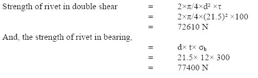
Since the least of the above two would be the rivet value, the rivet value in this case is 72610 N.
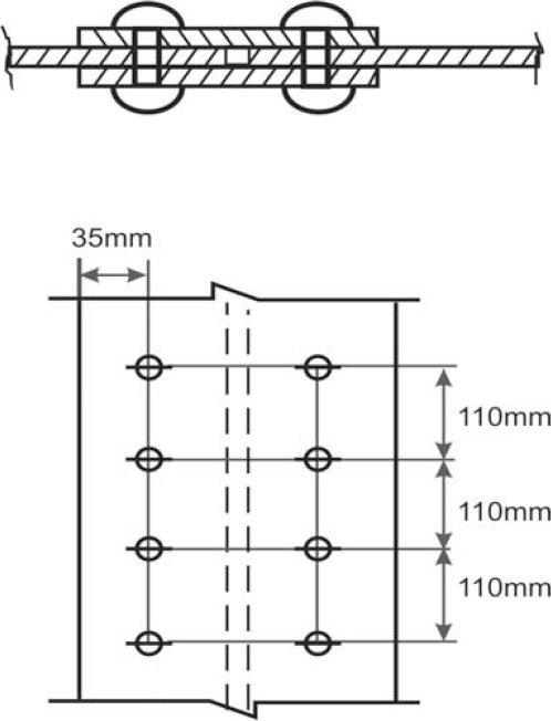
Details of a joint – illustration 6.2
For designing an efficient fastening, it would be the best situation if the post riveting strength of the plate equals the rivet strength. Since it is a continuous joint, covering a large width of the plate, we would compare the strength per pitch length, which would determine the value of the pitch (p). For this situation, the strength of plate per pitch length should be equal to two times the rivet value.
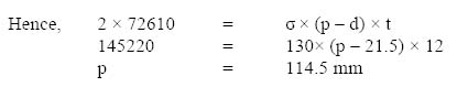
This is the upper limit of the pitch. Since the lower limit for pitch is 2.5 d (53.75 mm in this case), we would adopt the value of 110 mm for pitch.
Also, the edge distance should be minimum 1.5 d (32.25 mm); we would maintain the edge distance of 35 mm in this case.
The details of the joint are shown in Figure 6.7.
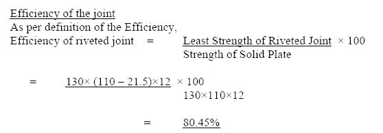
6.6.2 Design of bolted joints
As stated earlier, various types of fasteners are used for connecting the steel structural members. Different types of fasteners essentially serve the same function of transferring loads from one structural component to another. The choice of type of fastener is normally governed by the rigidity requirement, availability of technical inputs to fabricate and erect the structures, and service conditions for structure. In view of the ease in providing, bolted connections are preferred to riveted connections. In this case, the bolts along with nuts are used to fasten the components. In direct tension or compression members bolts act just like the rivets. For all other uses, unlike rivets, bolts form a semi-rigid connection. The failure conditions for bolts and the requirements related to pitch and minimum edge distance are the same as those for the rivets. The photograph of a typical bolted connection is shown in Figure 6.8.

Bolted joint: beam column
Quite similar to bolts are pinned connections, where pins are used instead of bolts. Normally if structures are subjected to shock or vibrations during service, for instance when they support machinery or dynamic loads, bolted connection is best avoided for critical structural connections. In such cases, pinned connections are preferred. They form flexible connections as far as rotation of the member at the joint is concerned. The pins are also used for hinged arches and similar other structures.
The advantages of bolted connections are as follows:
- Their application does not pose fire, heat or noise hazards.
- Bolted connections can be done much faster than any other connection.
- Bolted connections are economical to use due to requirement of lesser manpower, with low or moderate skills.
- Being a factory-finished product, the quality of the product is more assured.
At the same time, drawbacks in the case of bolted connections are as follows:
- The nut-bolt connection, being threaded, is suceptible to get loose. This can considerably reduce the load-transmitting capacity.
- The presence of threads results in reduced cross-sectional area and therefore reduced resistance to direct tension.
- The fixing requirement of holes with dimensional clearance causes vibration of structure.
Types of bolts
A bolt is a metal pin with a head formed at one end to retain it in position and the shank threaded at the other in order to receive a nut. The bolts used for structural purposes are manufactured from mild steel and have high strength steel. As described above, a bolt consists of a head and a body (or shank). Bolts are manufactured out of forgings in different lengths.

Parts of a nut and bolt
The size of a bolt is expressed by the diameter of the shank. The shank is provided with threads at the free end, where one or more nut can be fixed. To assure full grip between nut and bolt, the threaded portion of each bolt is dimensioned to project through the nut by at least one thread. The assembly is also provided with a washer of adequate thickness under the nut. A typical nut-bolt assembly is shown in Figure 6.9.
Structural bolts can be classified as follows:
- Unfinished bolts – Unfinished bolts, also termed as rough bolts or black bolts, are manufactured from low-carbon steel. The shanks of unfinished bolts are not uniform in diameter. Unfinished bolts are designed for a lower permissible stress in shear and bending in comparison to rivets and turned bolts. Unfinished bolts are not used for structural connections of members that are subjected to shock or vibrations. Unfinished bolts, generally, are used for temporary work or smaller loads.
- Turned bolts – Turned bolts are also termed fitted bolts, as these are forced fitted. Turned bolts are manufactured from forgings with hexagonal section. The bars are turned to required diameters. The threads in turned bolts are usually cut with a die. If the holes for the bolts are reamed, then for many situations the turned bolts can be treated, so as to have the same strength as rivets.
- High-strength friction grip bolts – The use of high-strength friction grip bolts or HSFG bolts is a relatively recent development in the field of steel structure fasteners. To act in the desired way, HSFG bolts are tightened to a predetermined shank tension that is equal to the proof load. Resultant to this, the structural elements connected together are clamped between the nuts and the head of the bolt. The load is transferred from one structural element to the other by friction between the parts. When the HSFG bolt is tightened, longitudinal tensile stress and torsional stress are developed in the shank of the bolt. The shank tension reduces slightly after completion of tightening. The torsion drops appreciably. Later on, the shank tension remains more or less constant for the whole of its working life, irrespective of whether the connections remain loaded or unloaded.
The bolts do not allow any relative movement between the connected elements. For HSFG bolts to act effectively, all the contact surfaces should be ensured free of scale, oils and other foreign material that could prevent perfect contact between the metals.
High-strength friction grip bolts have advantages over rivets and traditional bolts. Unlike these, the HSFG bolts are only subjected to uniform tensile stresses and no shear or bearing stress. These bolts have higher resistance against fatigue. Stress concentration in the bolthole remains absent. Also as HSFG bolts do not bear against the plates, the uneven distribution of stress does not occur.
Common terms in bolting
Some of the common terms related to bolts and their meanings are as follows:
Nominal diameter – The nominal diameter of a bolt is defined as the diameter of the shank prior to threading.
Gross area of the bolt –The gross area of a bolt is the cross-sectional area of the bolt, calculated from the gross diameter of the bolt.
Net area of the bolt – The net area of a bolt is the area at the root of the threaded part of the cross-section. Normally, it is taken as 75% to 80% of the gross area.
Diameter of the bolthole – The diameter of a bolthole is the nominal diameter of the bolt plus the clearance specified.
Bolt grip – The grip of a bolt is equal to the total thickness of the structural components to be held together. It is the distance between inside of the bolt head and inside of the nut, excluding the thickness of the washer, if any, in the tightened state of the bolt.
Length of the bolt – The length of the bolt is defined as the distance from the inside of the bolt head to the extreme end of the shank, including any camber or radius at the free end.
Effective interface – The effective interface is the common contact surface between the bolt and the connected members.
Permissible stresses in the bolts
The common bolts are categorized into two ways: (i) bolts turned as per close tolerance and (ii) bolts provided in the holes with sufficient clearances. For both categories, the permissible stress range for mild-carbon steel bolts is described in the table below.
| S N | Type of Stress | Range of Permissible Stress (N/mm2) |
| 1 | Tensile (σt) Close Tolerance Turned Bolts Bolts in Clearance Holes |
110–125 110–125 |
| 2 | Shear (τ) Close Tolerance Turned Bolts Bolts in Clearance Holes |
90–100 75–80 |
| 3 | Bearing (σb) Close Tolerance Turned Bolts Bolts in Clearance Holes |
280–300 240–250 |
In the case of high-strength friction grip (HSFG) bolts, the permissible loads in tension, for the different categories and diameters of bolts, are specified. In HSFG bolts, the permissible stress value for shear and bearing is less relevant since these bolts would generally not be subjected to these stress conditions.
Design of high-strength friction grip bolts
As stated earlier, in the case of HSFG bolts, the transfer of load from one member to the other is achieved through frictional resistance, along the contact surface of the members. The strength of the HSFG bolt joint is given by the following relationship:
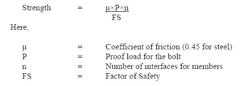
To ensure that HSFG bolts always remain in tension, they are tightened to a minimum prescribed level of torque. The nut and washer of the bolt remain in position by spring action due to tension in the bolt. As such, these nuts and washers do not become loose even if they are subjected to repeated variation of stress. There is also very little vibration in the tension of the bolt. The fatigue strength of the HSFG bolt is found to be 25% higher than the ordinary bolted or riveted connection. However, external tension is limited to 0.5 times the proof load so that separation of friction surface does not occur.
An illustration of the design of HSFG bolt connection is provided below.
Illustration 6.3: One 16 mm thick plate is to be joined by using 20 mm HSFG bolts. The proof load for bolt is 145 kN. The maximum permissible tensile stress for the plate material is 140 N/mm2. The pitch of the joint is 100 mm. It is required to determine the load-carrying capacity of the joint.
Let us consider the case of a butt joint. Two cover plates of adequate thickness have been used on either side of the 16 mm plate joint. This results into two interfaces where frictional resistance development takes place.
We also assume the coefficient of friction as 0.45 for the steel. The factor of safety adopted is 1.4.
As per the relationship observed earlier,
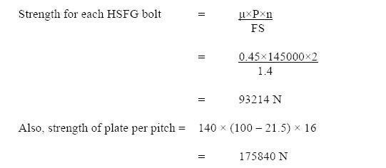
Out of these two, the lower value, i.e., 93214 N, is per pitch length strength or load-carrying capacity of the joint.
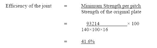
6.6.3 Design of welded joints
Welding is one of the effective methods of connecting two members of similar or different materials. In welding, a joint is developed between two pieces, by rendering their interface either plastic or liquid, by application of heat or pressure. This results into a permanent bond at the interface. A typical in situ welding process of steel structures is illustrated in the photograph in Figure 6.10.

Structure under welding
For structural steel fastening, welding is a widely used means. A typical weld for steel is shown in Figure 6.11. This type of weld is known as the groove or butt weld. The interface has been sloped or beveled to receive the filler metal. The zone in which the material has melted is termed as the fusion zone. The zone next to the fusion zone is the heat-affected zone. Although the metal in the heat-affected zone does not melt, its metallurgy undergoes a change due to the effect of heat received. The entire area consisting of filler, fusion zone and heat-affected zone together is known as the weld zone.

Weld-zone
The welding process may be used for joining metals other than steel too, provided it is economically feasible to do so. Mild steel, cast iron, copper, brass and aluminum can be welded by application of heat with or without pressure.
Various processes of welding
Different welding processes are described below in brief:
- Electric arc welding: It is one of the most widely used welding processes. In electric arc welding, heat is applied by means of an electric arc struck between the parts to be welded. The arc is generated by an electrode, which is held by a welder or an automatic machine. During welding, either the electrode itself melts and fills the gap at the joint, or the filler metal is fed separately into the arc. Besides generating an arc and supplying filler metal, the electrode through its coating supplies some important ingredients to the weld. This enhances the overall weld quality. Due to its versatility, electric arc welding is the most commonly used welding process for structural fabrication and erection works.
- Gas welding: In gas welding, the edges to be joined are melted by an oxyacetylene flame. This flame is generated by igniting the gaseous mixture of acetylene and oxygen in a specified ratio, through a specially designed welding torch. In the gas welding process, melting a welding rod in the flame generates the filler metal.
- Thermit welding: In thermit welding, a mixture of iron oxide and aluminum called thermit is ignited. Iron oxide, which gets reduced to molten iron metal, is then deposited at the joint by a mould constructed around the joint.
- Forge welding: This is essentially a pressure welding process. In forge welding, the interfaces of the segments to be joined are heated to the plastic state and then joined by applying an extremely high external mechanical pressure.
- Electric resistance welding: In electric resistance welding, the parts to be joined are pressed together and current is passed from one part to other. The resistance to the flow of current at the joint increases the temperature. When the temperature facilitating welding is attained, mechanical pressure is applied to forge the weld.
Advantages of welding
With the advent of welding, it has become possible to provide the perfect rigid joints in structures. The designer can be fully assured of it and can take this fact into consideration while designing structures. There is no loss of cross section of a member in a welded joint. In riveted and bolted joints, the cross-sectional area is reduced due to holes driven. Welded joints are capable of transmitting axial forces, shears and moments. The use of welding is increasing rapidly because of its several advantages over riveting. The advantages of welding are as follows:
- Welding is a noise-free process.
- Welding is a faster process in comparison to riveting.
- Welded joints have a better appearance than other types of joints.
- Welded joints provide more rigidity than riveted or bolted joints.
- Welding is more adaptable than riveting. In complicated structures, riveting or bolting may be extremely difficult or not possible but welding may be done easily.
- Welding is convenient for making additions in the existing structures.
- The efficiency of welded joints is higher than riveted or bolted joints, as in the case of welded joints, no holes are required to be made.
- Fastening by welding process, connecting angles, gusset plates, splice plates, etc., is not required. Thus, the overall weight of the structure doesn’t go up substantially.
- The cost of maintenance for a welded structure is low.
Disadvantages of welding
Besides the advantages that are described above, there are a few disadvantages associated with welding. These disadvantages of welding are described below:
- Uneven heating and cooling during welding may introduce distortions in the members.
- There is a greater possibility of brittle fracture in welding as compared to any other process of fastening.
- The process of quality control of a welded joint is expensive and complex.
- The skill sets required for welding are of a higher class.
- There is no option to prepare a joint that has flexibility of any degree.
Types of welded joints
The various types of welded joints are as follows:
- Butt weld
- Fillet weld
- Slot weld
- Seam weld
- Plug weld
In the case of butt or groove weld, the deposit of weld metal is done along the extended planes of the members. They are particularly useful if a member is subjected to direct forces. The weld acts as an extended part of the member and theoretically develops the full strength.
In fillet weld, the weld is formed outside the plane of the members. The weldment in this case would be subjected to either direct tensile or shear force.
The slot weld is a fillet weld, which is deposited along the periphery of a slot such that each of the perpendicular faces of the weld is formed through fusion in two separate structural members. If the weld is deposited along the outer periphery of a member, it is termed as seam weld.
Plug weld is made by filling the hole in a member such that the weldment also penetrates in the body of another member in contact.
Out of these, the butt weld joints and fillet weld joints are the most commonly used joints for structural purposes. The basic fillet weld and a few butt welds are shown in Figure 6.12.
Design of bull welded connections
The strength of a butt weld or groove weld is taken as equal to the strength of the parent metal, provided proper penetration of the weld metal is ensured. Out of the various types and shapes of butt welds, it is possible to ensure the penetration of the weld metal in the case of double-V, U, J and double-bevel joints, as the shape of the joints allows weld metal deposition from both faces of the joints. The permissible stress for the weld is taken to be the same as for the parent metal.
However, in the case of single – V, U, J and single-bevel joints, the weld penetrations generally remain incomplete. Due to this, the effective throat thickness for these types of joints is taken as 5/8 times the thickness member. In case the thickness of the two joining parts is different, the thickness of the thinner part is considered for the purpose of calculation of strength.
In the case of joining of two parts of unequal thickness, it is crucial to properly design the weld joint. In case the difference in thickness is more than 25% of thickness of thinner part or 3 mm, it is necessary to provide a taper, usually not more than 1 in 5, to ensure gradual change in the thickness.

Types of welds
Another important aspect is the selection of a proper sized electrode for welding. The diameter selected should be such that the resultant arc should be able to reach the root or the neck of the butt joint.
Design of fillet weld joints
As described earlier, the fillet weld is the deposit of weld metal outside the projected planes of the members. This is the single most important factor, which differentiates fillet welds from butt welds. The cross section of the fillet weld is triangular, as shown in Figure 6.13.
Some of the important terms, used while designing a fillet weld, have been described as follows.
Size of the fillet weld: The length of the sides of the largest right-angled triangle in the cross section of the fillet weld is denoted as the size of the fillet weld. Usually, the perpendicular sides of such a right-angled triangle are equal and the size of a fillet weld may be specified in one dimension only.
The minimum size of the fillet weld is usually specified on the basis of the thickness of the parts to be joined. The indicative sizes for different thickness ranges are specified, in the table below:
| Thickness of Thicker Part | Minimum Fillet Weld Size |
| Up to and including 10 mm | 3 mm |
| Over 10 mm up to and including 20 mm | 5 mm |
| Over 20 mm up to and including 30 mm | 6 mm |
| Over 30 mm up to and including 50 mm | 8 mm first run 10 mm minimum |

A fillet weld
The maximum size of the fillet weld is also specified. The maximum size of the fillet weld applied to the square edge of a plate or member should be 1.5 mm less than the nominal thickness of the member or edge. The size of the fillet weld used, along the toe of an angle or the rounded edge of a flange, should not exceed three-fourths the nominal thickness of an angle or flange leg.
Throat of fillet weld: The throat of a fillet is the length of the perpendicular, from the right-angle corner to the hypotenuse, as shown in Figure 6.11. The effective thickness of throat is dependent on the size of the fillet, as well as the angle between the edges to be joined. The throat can be calculated with the following expression:
Throat Thickness = K × Fillet Size
In most of the cases, a right-angled fillet is formed during welding. For this case, the size of throat is equal to the 1/√2 times the size of the fillet. For this case,
K = 1/√2 = 0.7
Effective length of fillet weld: The effective length of a fillet weld is equal to its overall length minus twice the weld size. This is considered as the length that is truly effective in withstanding the load. This reduction from actual length takes care of the weld imperfections, at the start and at the end of the weld. The effective length of a fillet weld, designed to transmit loading, should never be less than four times the weld size. The length shown by the designer on the drawing is the effective length for the weld. The welder is supposed to provide the additional length (i.e. 2 x weld size) of the weld.
End return: The end return is the precaution about termination of weld at the end of the member. The fillet weld terminating, at the end or side of a member, should be returned around the corner, whenever practicable, for a distance not less than twice the weld size. This provision applies, in particular, to fillet welds in tension connecting beam seating, brackets, etc.
Side fillet: Side fillets are separate rows of fillet welds for the same member. These are designed to resist the force in combination with each other. For a lap joint made by a side or longitudinal fillet weld, the length of each fillet weld should not be less than the perpendicular distance between them. The perpendicular distance between the side fillets should also not exceed sixteen times the thickness of the thinner part connected. In case this limit cannot be adhered to, an additional end fillet plug or slot weld is provided to prevent buckling or separation of the parts.
Intermittent fillet weld: Intermittent or discontinuous fillet welds may be used when the length of the smallest-size fillet weld required to transmit stress is less than the continuous length of the joint. As stated earlier, any section of an intermittent fillet weld should have an effective length of not less than four times the weld size. The clear spacing between the ends of the effective lengths of intermittent fillet-weld carrying stresses should not exceed 12 t for compression and 16 t for tension, where t = thickness of thinner part joined, and in no case should be more than 20 cm.
Chain intermittent welding, where the weld length and gaps have a regular pattern, is to be preferred to irregular intermittent welding. When staggered intermittent welding is used, the ends of the component parts should preferably be welded on both the ends.
Single fillet weld: The single fillet weld is a single line of fillet welds. When single fillet weld is used, it should not be subjected to bending about its longitudinal axis.
Permissible stress and strength of fillet weld
As we can visualize, the fillet weld may be subjected to two types of loads. In the first case, which is the most frequent one, the members can be subjected to tension where the load would act along the longitudinal axis of the weld. In such cases, the weld metal would be subjected to direct shear force. Both the perpendicular edges being fused with the different members would tend to move in the different directions. This would cause the weldment to slide longitudinally along its weakest section.
In the other case, the direction of load can be in transverse direction to the weld axis. In such cases, the weld would be termed as ‘in tension’ and the rupture again would be along the smallest length of the cross section.
Fillet welds are designed for shear stress at its minimum section, i.e. the throat of the weld. The permissible stress in the fillet weld is 105–115 N/mm2. The shear strength of a fillet weld is given by the following equation:
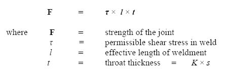
Since for most of the cases the angle between the welded surfaces for fillet weld is either 90º or very close to it, the value of K can be adopted as 0.70.
Hence, t = 0.7s
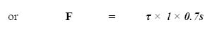
The values of permissible stresses, in shear and tension, are reduced to 80% for field welds made during erection.
To explain the process of fillet weld design in detail, following illustration has been used.
Illustration 6.4: Two 200 mm wide steel plates of 10 mm thickness each are to be fastened together with a 6 mm sized fillet weld. If the total weld length is 200 mm and the permissible shear stress in the weld metal is 115 N/mm2, we need to determine how much load can be safely transferred through the arrangement.
As is obvious, the total load transferred can be lower than the capacity of the plates under tension and the weld capacity under shear. Since the plates have been as wide as the total length of weld, substantially thicker than the weld size, and steel’s capacity to withstand tension is higher than its capacity to withstand shear, the weld’s capability to transfer load would be the limiting capacity of the overall arrangement.
For a 900 fillet weld, the capacity to withstand force is given by the following relationship:
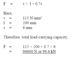
Illustration 6.5: The objective is to design a lap joint for two plates of 8 mm and 12 mm thickness respectively. The width of each plate is 150 mm. The values of permissible stresses are as follows:
for plate in tension – 145 N/mm2
for weld metal in shear – 110 N/mm2
The arrangement of the joint is shown in Figure 6.14.
Since the plates have equal width, the smaller of the two thicknesses, i.e. 8 mm, would determine the design of the joint.
As per norms, the overlap between the two plates should not be less than five times the thickness of the thinner plate. Hence the length of overlap
= 5 × 8 = 40 mm
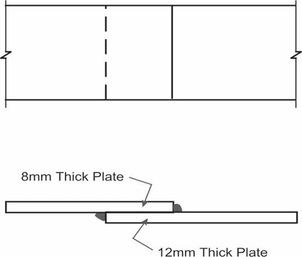
Lap welded joint –illustration 6.5
As already stated, the strength of the thinner plate would govern the design of the weld joint. The tensile force carrying capacity of this plate is as follows:

This force of 174000 N would be shared by the two lengths of fillet welds, each of 150 mm. If the forces shared between them are T1 and T2 respectively, then

Since both the plates would elongate together, the value of elongation in both should be same for the overlap length. To satisfy this condition,
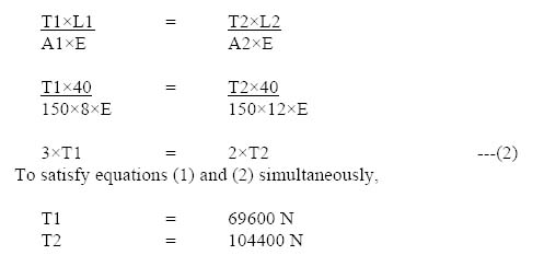
Since both the welds are 90º fillet welds, the size of each can be determined by the following relationships:
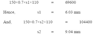
Since the maximum weld size should be smaller by at least 1.5 mm from the member thickness or the edge size, we can adopt fillet weld of size 6.5 mm and 10 mm respectively for the 8 mm thick and 12 mm thick plate, respectively.
Design of eccentrically loaded fillet weld joint
In day-to-day work, designers come across problems when the welded joint is subject to eccentric loading and, consequently, the moment. For instance, consider the case of the bracket shown in Figure 6.15. The bracket has been welded with the column flange through fillet weld of size s. The depth of the bracket, as well as the length of each run, of weld is equal to d.
As shown in the diagram, a concentrated load of magnitude W has been acting on the bracket. The load is eccentric with respect to weld axes by distance e. Under this situation,
Total length of weld = 2d
Vertical shear stress in the weld (pv) = 

Example of a bracket
The eccentric loading would also cause bending moment in the fillet weld. The value of this moment M is equal to W×e.
Magnitude of the horizontal shear stress due to bending in the extreme fibre,
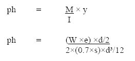
With the help of these determined values of pv and ph, the value of resultant stress can be determined by the following relationship:
Resultant Stress (pr) = √ (pv2 + ph2)
The value of the resultant stress should not exceed the permissible value of shear stress in the weld material.
This has been explained with the help of an illustration below.
Illustration 6.6: The objective is to determine the size of the fillet weld to fix a bracket plate of 12 mm thickness with the column. The size of the bracket, load intensity and its eccentricity are shown in Figure 6.16. The permissible stress for weld metal in shear has been 110 N/mm2.

Design of fillet weld – illustration 6.6
Let’s begin with the assumption that the weld size is s mm.
Vertical Shear Stress, pv = 75000 / (600×0.7s) = 178.57/s.
Total Moment due to eccentricity, M = 75000 × 300 = 22500000 N-mm.
Horizontal shear stress at extreme fibre due to bending moment
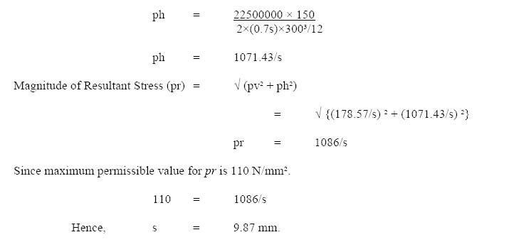
Therefore, we can provide 10 mm sized fillet welds. Since the plate thickness is 12 mm, this weld size would be fully acceptable.
6.7 Design of tension members
A structural member, subjected to tensile force, in the direction along or parallel to its longitudinal axis is termed as tension member. A tension member is also described as a tie member. The term tie is commonly used for tension members in the trusses. Wire cables, circular, square and flat bars are the simplest forms of tension members in use for light bridges and roof trusses. When a member is subjected to axial tensile force, the distribution of stress over the cross section becomes uniform. The entire net cross-sectional area of the member is effectively used at the maximum permissible uniform stress. Therefore, a tensile member subjected to axial tensile is said to be an efficient and economical member.
Since the structural member used for fabrication and erection is not perfectly straight, the initial crookedness and imperfections of the member result in the small eccentricity of loading. The distribution of stress in the eccentrically loaded tension member would not be uniform and the member would be subjected to combined stress (i.e., direct tension and bending). A tension member may also intentionally be subjected to combined axial tension and bending.
6.7.1 Types of tension members
A tension member is defined as the structural component subjected to tensile force. Steel is one of the best construction materials, which has a good capacity to bear tensile stress. The nature of the structure, magnitude of stress and the method of connection govern the selection of tension member. To the possible extent, efforts are made in the case of tension members to connect them directly to gusset plates or splice plates. This helps in minimizing the possibility of stress concentration in the members.
The various types of tension members used may be grouped as follows:
- Wires and cables
- Rods or bars
- Rolled structural sections
- Built-up members
Wires and cables: Wire ropes and cables are used as tie members in the case of low-stressed or temporary applications such as hoists, derricks, rigging slings, guy wires, etc. Untwisted parallel wires are used in the manufacture of main cables of suspension bridges. Wire ropes have the advantages of flexibility and strength. At the same time, they require specially designed fittings for proper end connections as traditional structural fasteners can be of little use. Wire ropes are initially stressed when used as guy ropes for steel towers. This initial tension prestresses the frame due to which the effectiveness of the frame in resisting the external load is increased.
Rods or bars: Square and round bars are frequently used as tension members. To facilitate jointing, round bars are threaded at the ends and are used with nuts. Often, instead of providing threads, the bars are bent to form loops at their ends. Round bars with clevises as well as loop rods are made in two portions. These portions are joined and tightened with the help of turnbuckles. Such members are commonly used for lateral bracing. In the case of rectangular section bars and small width flats, the ends are enlarged by forging and holes are driven in them to form eye bars. These eye bars are used with pin connections. Inadequate stiffness of rods and bars results in noticeable sag under self-weight.
Rolled structural sections: A variety of rolled structural sections, viz. angle sections, tee sections, channel sections, etc., are used as tension members in structures. Angle sections have considerably more rigidity as compared to wire ropes and bars. Angle sections are also widely used for the purpose of bracing. A single-angle section develops bending stress due to the eccentricity between the end connections and the centre of gravity of the angle section. Unlike ropes and bars, these members can also resist some compression if reversal of stress takes place. Channel sections can also be effectively employed as tension members. Occasionally, I-sections are also used as tension members. These sections have the advantage of a high level of rigidity.
Built-up members: Built up members are the combination of either more than one rolled sections fastened together or a combination of one rolled section along with plates, or a section developed only with the plates. When single rolled steel sections cannot fulfill the requirement of cross-sectional area, built-up sections are used. Obviously, members constructed with built-up sections are used in the case of heavy tensile force. Built-up sections are normally designed as more rigid and stiffer than single rolled structural sections. As built-up sections are custom made, the sectional properties, such as total area, moment of inertia, etc., are properly controlled. These sections can resist compression force if the reversal of stresses takes place in the structure.
Some commonly used built-up sections are shown in Figure 6.17. Double-angle sections, placed back-to-back, with equal or unequal legs are extensively used as tension members in the roof trusses. Two angle sections may be arranged in the star shape, with the diagonals opposite each other and with legs on the outer sides. The star arrangement provides a symmetrical and concentric connection. Two angle sections have the advantage of adjusting the distance between them. Four angle sections are also used in the large biplanar trusses. A built-up section may be made of two channels, placed back-to-back, with a gusset plate between them. Such sections are used for medium force in a single-plane truss. In bi-planar trusses, two channels are arranged at a distance with their flange turned inward. It simplifies the transverse connections and also minimizes lacing. The flanges of two channels are occasionally turned outward in order to have greater lateral rigidity. The heavy built-up tension members in the bridge truss girders are made of angles and plates.
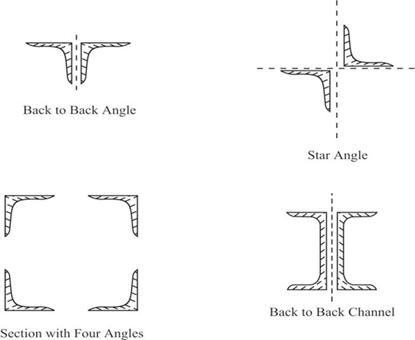
Commonly used built-up sections
Determination of net cross-sectional area for tension members
As is quite obvious, if a steel section has been fastened by drilling holes as is the case with rivetting and bolting, it would not be possible for the member to transfer the tensile force to those fasteners. In such cases therefore, the net or effective area resisting tensile force would be less than the gross cross-sectional area. The net cross-sectional area of a tension member is the gross cross-sectional area of the member less the deductions made for holes. The projected area for each hole would be a rectangle: one side of which would equal the thickness of the member and the other side would equal the diameter of the hole.
Let us examine the case of some specific sections and the ways to apply deductions to them.
Plates: In the case of plates, the pattern of holes for fasteners determines the amount of deductions.
- For chain riveting or bolting, the net area of the member at cross section is the gross cross-sectional area less the area to be obtained from the product of thickness of the plate and the sum of the diameters of all rivet and bolt holes in that section.
If the plate has a thickness t and width b, the gross diameter of holes is d and the section has n such holes,
Anet = t × (b – n×d)
- If fasteners are placed in a zig-zag fashion, the failure of a plate may occur along this zig-zag section and would pass through these fasteners instead of a straight section, passing through the section, with higher numbers of fasteners. When one or more than one hole falls off the line, the failure of the plate depends upon the staggered pitch (p), gauge distance (g), and the diameter of the hole (d). When the gauge distance is larger than the staggered pitch, the failure may occur in zig-zag line. When the gauge distance is small, as compared to the staggered pitch, the failure may occur along a straight right angle section, passing through the largest number of holes. In case both the staggered pitch and the gauge are similar, the probability of the zig-zag failure occurring increases considerably as the diameter of the hole increases.

Net c/s area for tension member
From theoretical investigations and laboratory tests, it is found that the net area of the plate for such a section would be the actual net area calculated along the zig-zag section plus additional area calculated from the following expression:
Additional Area = p2×t/4g
In case the rivets are connected in different staggered pitches p1 and p2 and the gauge distances g1 and g2, as shown in Figure 6.18, the net area along the section ABCDE shall be
Anet = t × {b – n×d + (p12×t / 4g1 + p22×t / 4g2)}
Angles and tee-sections: When an angle section is used as a tension member, it is connected with the gusset plate by one leg. When a tee section is used as a tension member, it is generally connected with the gusset plate by its flange. In such cases, the rivets connecting the tension member and the gusset plate do not lie on the line of action of the load, the result of which is an eccentricity moment on the connection. The distribution of stress becomes non-uniform because of eccentric connection. The net cross-sectional area of an angle or a tee member is reduced to account for this non-uniform distribution of stress. The reduced net cross-sectional area of such members is called net effective area.
Some commonly encountered situations are shown in Figure 6.19. The value of net effective areas for different situations is as follows.

Typical sections for tension members
- For a single angle connected by one leg only – The net effective area for this situation would be as per the following expression:
Anet = A1 + A2 × k1
Here, A1 = Net cross-sectional area of the connecting leg
A2 = Gross cross-sectional area of the other leg
k1 = 3× A1 / (3× A1 + A2)
- For two angles connected back-to-back or single tee – The net effective area for this situation would be as per the following expression:
Anet = A1 + A2 × k1
Here, A1 = Net cross-sectional area of the connecting legs of angle or of flange of tee
A2 = Gross cross-sectional area of the other legs or of web of tee
k1 = 5× A1 / (5× A1 + A2)
- For two angles connected back-to-back or two tees connected to each side of the gusset – The net effective area is calculated by reducing the area of the holes from the gross sectional area, provided the members are tack-fastened along their length. In case they are not tacked together, each would be considered as an individual section on one side of the gusset and the area would be determined accordingly.
However, if staggered fasteners are used in two legs of an angle section, then the net area would also be determined by the provisions for zig-zag fastening.
Allowable tensile stress in steel
When a steel structural member is subjected to direct tension, the requirement is that the maximum stress in the section should be limited to 60% of the guaranteed yield stress for the metal. The stress calculation is done on the basis of net area of the section.
Hence, permissible direct tensile stress,
σtd = 0.6 × fy
Steps in design of axially loaded tension member
The below steps are followed while designing an axially loaded tension member:
- Determine the total load for which the member has to be designed.
- Calculate the net sectional area required as –
Required Anet = Total force / Permissible tensile stress
- Conduct a trial with a suitable section, with a gross sectional area 20% to 30% larger than the Anet calculated. If a selection has to be made out of rolled sections, the sectional area and other properties of these sections are obtained from the relevant design codes and tables.
- The next step would be to calculate the Anet available in this trial section. At this stage, the following deductions for fastening holes may be assumed as a thumb rule:
- For plates – one rivet hole for each 150 mm width
- For single angle or double angle – one rivet hole from each angle
- Double channel – two rivet holes from each channel web or one rivet hole from each flange
- If Anet for this section is equal to or more than the required net area, the section can be adopted.
- As a special case, if the nature of loading on the member is such that the reversal of stress can occur during the life span, it would be necessary to calculate the slenderness ratio and verify its meeting norms.
- The final step in the process is to design the end connections.
The process of determination of net effective area for the tension members and the influence of different factors on it are shown in the illustration below.
Illustration 6.7: We need to assess the tension-carrying capacity of the member. As shown in Figure 6.17, the flat of size 175 mm × 12 mm has been used as a tension member. Its connection to another member is through a gusset plate of adequate size and strength. The fastening is through 20 mm nominal diameter rivets. The proposed arrangement of rivets is as per the diagram. The yield strength of steel is 250 N/mm2.

Design of tension member with gusset – illustration 6.7
For this situation,
Diameter of holes = Gross diameter of rivets = 20 + 1.5 = 21.5 mm
Permissible tensile stress = 60% of 250 N/mm2 =150 N/mm2
As per the rivet arrangement, this is the area number of potential failure sections. We need to separately examine each to determine which section offers the least area and to resist the tensile force. We will convert all the dimensions into cm.
Section 6-5-7:
This section has one rivet hole. As the gauge is smaller than the staggered pitch in this case, the influence of the nearby holes will not be felt:
Anet = 1.2×(17.5 – 1×2.15) = 18.42 cm2
Section 1-2-3-4:
The section has two rivet holes. At the same time, the strength is additional due to existence of rivet ‘5’. In this case, the net effective area would be
Anet = t × {b – n×d + p2/ 4g}
Anet = 1.2× {17.5 – 2×2.15 + 52 / 4×4} = 17.71 cm2
Section 1-2-5-7:
The section has two rivet holes. Apart from the reduction in effective area due to these, there will also be strength provided by rivet ‘3’. In this case, the net effective area would be
Anet = t × {b – n×d + p2/ 4g}
Anet = 1.2× {17.5 – 2×2.15 + 52 / 4×4} = 17.71 cm2
Section 1-2-5-3-4:
This section has three rivet holes within it. Apart from the reduction in effective area due to these, there would also be strength provided by two rivets. In this case, the net effective area would be
Anet = t × {b – n×d + 2×p2 / 4g}
Anet = 1.2× {17.5 – 3×2.15 + 2×52 / 4×4} = 17.01 cm2
Of the entire scenario examined, the least effective area emerges as 17.01 cm2 or 1701 mm2. This is the critical area for the arrangement.
Since the permitted tensile stress for the section is 250 N/ mm2, the maximum tensile load-carrying capacity would be as follows:
T = 1701 × 150 = 255150 N or 255.15 kN
Illustration 6.8: An angle section of size 75 X 75 X 8 mm has been used as a tension member. One leg of the member has been bolted to the gusset plate with 16 mm bolts in a single row. The objective is to determine the tensile force-carrying capacity of the member. We also need to determine the maximum tensile load that can be carried through this section. The yield strength of steel is 250 N/mm2.
For this situation,
Diameter of bolt holes = 16 + 1.5 = 17.5 mm
Permissible tensile stress = 60% of 250 N/mm2 =150 N/mm2
Though the angle section will have an actual thickness of varying degree, we would consider it as a section with parallel and perpendicular edges, without any curvatures. The precise geometry of the section and its area statement can be obtained from the relevant codes. The sketch of the angle section and arrangement is shown in Figure 6.21.
We already know that in the case of a single-angle tensile member with holes driven into it, the net effective area would be given by the following expression:
Anet = A1 + A2 × k1
Here, A1 = Net cross-sectional area of the connecting leg
A2 = Gross cross-sectional area of the other leg
k1 = 3× A1 / (3× A1 + A2)

Design of tension member – illustration 6.8
Hence, area of each leg of the angle,
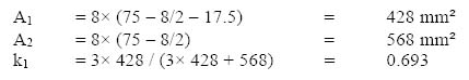
And, Anet = 428 + 568 × 0.693 = 821.6 mm2
Based on this net area, the maximum tensile load-carrying capacity of the member,
T = 821.6 × 150 = 123240 N or 123.24 kN
To determine the maximum possible tensile load-carrying capacity of the member, the holes for any fasteners would require to be eliminated. The member would be fixed to the gusset through welding and, therefore, no loss in the gross cross-sectional area would take place. We also assume that the weld design has been done to take care of the eccentric center of gravity of the angle section, and no moment is induced in the section.
In this case, overall cross-sectional area = 2× A2 = 2× 568 = 1136 mm2
Overall tensile load-carrying capacity in this case,
T = 1136 × 150 = 170400 N or 170.4 kN
It may be observed here that the reduction in load-carrying capacity of a member is due to holes. In this case, it is about 27.6%.
6.8 Design of compression members
A compression member is defined as the structural component subjected to compressive force in a direction parallel to its longitudinal axis. The terms stanchions, struts and posts are also used for compression members. Columns, stanchions and posts are general terms used for vertical compression members in building construction. The term strut is commonly used for compression members in trusses. A strut may be used in a vertical position or in an inclined position in roof trusses. Compression members may be subjected to both axial compression and bending.
When compression members are loaded beyond their capacity, their failure may take place because of one of the following reasons:
- Direct compression or crushing
- Excessive bending
In the case of bending in the columns, the failure load of a column is a function of its slendemess ratio. In fact, except for very short columns or stub columns, bending would always be present in the case of compression members. Its reasons and effects have already been discussed in the earlier section. The cross-sectional area of the member being constant, the magnitude of load required to cause bending failures in a compression member decreases as the length of the member increases. Therefore, columns are also classified as short and long.
Axially loaded columns
In an axially loaded column, the load is applied at the centroid of the cross section and it acts in the direction parallel to the longitudinal axis of the column. The term concentrically loaded is also used to specify axially loaded columns.
An axially loaded column can be defined as the one which transmits only compressive force, with no explicit design requirement to withstand either lateral loads or end moments. However, a perfectly straight column with central application of load is an ideal condition. During fabrication and erection of structural columns, it is difficult to avoid accidental eccentric load application, crookedness and curvature, and the presence of residual stresses. The effect of these is to reduce the overall load bearing capacity that can be addressed by making appropriate modifications in the analytical expressions and using suitable factors of safety in the design formula.
At this stage, we should review our earlier understanding about the phenomenon of critical loads for a column, which we had studied in the section on column analysis. Consider the case of an ideal column, which is vertically fixed at the base and free at the upper end and subjected to an axial load F. The column is assumed to be perfectly elastic. When the value of load F is less than the critical load and stress is within the limit of proportionality, the column remains straight. In this stage, the column is said to be in stable equilibrium. This means that if a small lateral load is applied at the free end the column deflects and the free end moves laterally. However on withdrawal of the lateral load, the column resumes its vertical position and deflection vanishes. When the axial load F is gradually increased, a stage would eventually be reached when the column would attain the position of unstable equilibrium. At this stage if a small lateral load is applied, the resultant lateral deflection will not disappear on withdrawal of this lateral load. The magnitude of minimum axial load required to keep the column in such a deflected shape is termed as critical load. Critical load is also called buckling load or crippling load.
Buckling is the sudden bending or warping of the members under compressive load. Buckling load is the load at which a member buckles and, consequently, fails functionally. The direction of buckling of a column depends upon flexural rigidity, El, of the column section. The compression member buckles in a direction perpendicular to the axis, about which the moment of inertia of the section is minimum.
Euler, a Swiss mathematician, had derived one of the most widely used expressions for the critical load for columns. This is known as Euler’s column formula:
Critical Load, Fcr = 
Here, E = Modulus of elasticity of the material
I = Least moment of inertia of the column cross section
Leff = Effective Length of the column
Effective length of the compression members
The effective length of a compression member depends upon the end restraint conditions. These end restraints are of two types:
- Restraints for position : In position restraint the end of the column is not allowed to shift from its position, but is permitted to rotate. The example of this is the hinged connection.
- Restraints for rotation: In rotation restraint the end of the column is free to change its position, but is not allowed to rotate.
A column end can be free or can have either one of the restraints. It can also be subjected to both the restraints. The end conditions of the column determine its effective length, which has a bearing on the value of critical load for the column.
There are various possible combinations of restraints about either or both axes. The restraint conditions at the two ends of a column can remain same or can differ. Given below are some standard cases of end conditions:
- Both ends of column hinged
- Both ends of column fixed
- One end of column fixed and the other end hinged
- One end of column fixed and the other end free
The representative diagrams, for a number of such end restraint conditions, are shown in Figure 6.22.
In all the cases, the actual length of the column is L. Case 1, i.e., both ends of the column hinged, has been considered as a standard case. The effective length (Leff) of a column is expressed in terms of equivalent length of compression members hinged at both the ends. The equivalent length can be defined as the length of a column between two adjacent points of zero moments, and is represented by L. It is also termed as unsupported length.

Effective column lengths – schematic diagram
The effective length of a compression member can be adopted as per the table given below. Although the perfect end conditions, assumed in the analysis, are nearly impossible to get in practice, the values of effective lengths indicated in the table will be accurate enough for most cases. These values of effective length can also be adopted if the columns form part of the framed structures.
| Types of End Constraints | Effective length of the member (Leff) |
| Effectively held in position and restrained against rotation at both ends | 0.65 L |
| Effectively held in position at both ends and restrained against rotation at one end | 0.80 L |
| Effectively held in position at both ends but not restrained against rotation | 1.00 L |
| Effectively held in position and restrained against rotation at one end and at the other end restrained against rotation but not held in position | 1.00 L |
| Effectively held in position and restrained against rotation at one end and at the other end partially restrained against rotation but not held in position | 1.5 L |
| Effectively held in position at one end but not restrained against rotation, at the other end restrained against rotation but not held in position | 2.00 L |
| Effectively held in position and restrained against rotation at one end but not held in position or restrained against rotation at the other end | 2.00 L |
Important sectional properties for compression members
Effective cross-sectional area for compression member: In the case of compressive load, a member can also transfer the load to the fasteners. Therefore, the effective cross-sectional area of a compression member is the gross cross-sectional area of the member. No deduction is made for holes meant for rivets, bolts and pins, as long as the fasteners fill them. However, the plate element or outstand of a section may buckle under the compressive force before the failure of the entire member. To avoid this, the effective area is modified when the ratio of the outstand to thickness exceeds the limits specified. The outstand in the case of channels and angles is measured as nominal width of the sections. In the case of flanges of beams and tee section, it is measured as half the nominal width. The outstand for a number of sections is shown in Figure 6.23.
The thickness is taken as 1/16 of outstand of any member in compression for unstiffened outstand and 1/20 of outstand of any member in compression for stiffened outstand. The thickness is taken as 1/90 of outstand for unsupported width of unstiffened plate forming any part of a compression member, measured between an adjacent line of rivets. But for the purpose of calculating effective cross-sectional area and radius of gyration, only 50 times the thickness of plate will be taken, instead of 90 times the thickness, in case a single plate is used. However, it is the total thickness of two or more plates effectively tacked together.

Outstand of typical rolled sections
A deduction is also made from the gross cross-sectional area for excessive effective plate width (if any) to determine the effective sectional area.
Radius of gyration: The radius of gyration of a section is a geometrical property of the section and it is denoted by r. The expression for this has been
r = √ (I/A)
where I = Moment of inertia of the section about the axis
A = Effective sectional area of the section
Slenderness ratio: The slenderness ratio of a compression member is defined as a ratio of effective length of compression member (Leff) to appropriate radius of gyration (r).
Slenderness ratio, λ = Leff lr.
The slenderness ratio of a compression member should be as small as possible, so that the material may be stressed to its largest permissible limit. In the case of rolled steel sections, the values of I, A and r are obtained from the design tables, which provide details of sectional properties. The radii of gyration about various axes of rolled steel sections can be obtained from structural steel section tables. The minimum value of radius of gyration gives the maximum value of slenderness ratio. For built-up compression members, the value of radius of gyration is calculated independently.
The end restraints of columns are often different in the two principal planes. The different values of moments of inertia of the column cross section in these planes are sometimes beneficial to achieve approximately equal slenderness ratios in both the planes of bending.
Compression members composed of two sections
As we have seen in the case of Euler’s formula, the value of critical load for a section depends upon the moment of inertia of the section. Incidentally, as per Euler’s formula, the value of critical load is independent of the sectional area. In the case of other column formulae too, the overall sectional properties determine the value of critical load. Hence, it sometimes becomes important to enhance the sectional properties of a rolled section by using it in combination with plates or other sections. One of the most effective and efficient ways would be to form a new section by placing two similar rolled sections back-to-back. This process necessitates certain norms which should be followed to ensure that the two different sections work as one.
- A compression member with two similar sections back-to-back, either in contact or separated by a small distance, should be joined together by riveting, bolting or welding so that the slenderness ratio of each member between the connections is neither greater than 40 nor greater than 0.6 times the most unfavorable slenderness ratio of the whole strut. The spacing of tacking rivets in a line should not exceed 600 mm for such members.
- For other types of built-up compression members, where, say, cover plates are used, the pitch of tacking rivets should not exceed 32 t or 300 mm, whichever is less (where t is the thickness of the thinner outside plate).
- The rivets, bolts or welds in these connections should be sufficient to carry the shear force and moments, if any specified for battened struts. The diameter of the connecting rivets should not be less than the minimum diameter given below.
| Member Thickness | Minimum diameter of rivets |
| Up to 10 mm Over 10 mm but up to 16 mm Over 16 mm |
16 mm 20 mm 22 mm |
- The ends of the struts should be connected together with not less than two rivets or bolts or their equivalent in welding and there should not be less than two additional connections spaced equidistant in the length of the strut.
- A minimum of two rivets or bolts should be used in each connection: one on each line gauge mark, where the legs of the connected angles or the tables of the connected tees are 125 mm wide or over or where the webs of channels are 150 mm wide or over.
Load bearing capacity of compression member
The strength of a compression member is defined as its load-carrying capacity. The strength of a centrally loaded straight steel column depends on diverse factors like effective cross-sectional area, radius of gyration (viz., shape of the cross section), the effective length, the magnitude and distribution of residual stresses due to heat treatment and cold straightening, etc. The importance of all these factors is of varying degree.
The effective cross-sectional area and the slendemess ratio have high significance for a compression member. The permissible stress for the member is dependent on the slenderness ratio. Once the value of slenderness ratio is known, the permissible stress for a particular steel grade can be determined either from design charts or from graphs. A typical graph for the purpose is shown in Figure 6.24. Other factors described above are of relatively lesser importance.

Relationship between slenderness ratio and permissible stress in columns
The steps involved in determining the safe bearing capacity of a compression member are as follows:
- First of all, one needs to determine the effective length from the actual length of the compression member and the end support conditions.
- With the section of the compression member known, the radius of gyration about various axes of the section either has to be calculated or to be directly read from steel section tables. The least value of the radius of gyration is adopted for the analysis.
- With effective length and radius of gyration known, the maximum slendemess ratio (L/r) is determined for the compression member.
- The allowable working stress (σcd), in the direction of compression, is seen from the table, corresponding to the maximum slendemess ratio of the column and the grade of the structural steel.
- The effective sectional area (A) of the member is noted from structural steel section tables. For the built-up members, it can be calculated.
- With the values of effective area and permissible stress known, the safe load-carrying capacity of a member is determined from the relation
F = A × σcd
In case the objective is to design a section, for the compression member, capable of withstanding a particular magnitude of load safely, the steps would be as follows:
- As the actual length of member and end conditions for the supports are known, the effective length of the member would be computed first.
- It would be required to assume a value for safe stress in the steel. As a thumb rule, for a low-load case where a single rolled section is going to be adopted, a stress value corresponding to slenderness ratio of around 100 can be assumed. For a high-load cum built-up section scenario, the value of stress corresponding to a slenderness ratio of 60 -70 may be assumed at that stage.
- With the value of permissible stress assumed, the next step is to work out the cross-sectional area requirement for the given load.
- With the target cross-sectional area known, a trial section (single or built-up) would be developed at this stage. For this section, the radius of gyration and actual slenderness ratio would need to be determined.
- The permissible stress for this permissible ratio would be read from the chart /table.
- The safe load for the trial section would be determined and compared with the actual load value. In case the actual exceeds the computed load, a fresh trial with a further enhanced section would need to be made.
Built-up compression members
We already know that the load-carrying capacity of a compression member is dependent on its slenderness ratio, which in turn is dependent on the member’s effective length as well as the moment of inertia of its cross section. To put it in another way, the load-carrying capacity of a compression member of a given material and fixed effective length is the function of the moment of inertia of its cross section. Therefore, the distribution of the material in the cross section is quite important. In the cases of heavy compression loads, built-up sections (sections made of two or more sectional members/plates) are provided. While designing such a section, an effort is made to place the material uniformly with respect to both the major axes of the cross section and also to space it as far from the centre as possible.
To ensure that the different components of the built-up section act as a single column, it is necessary to connect them. These connections are designed to withstand all the forces, which try to separate the components. This connection is achieved either by lacing or battening. In lacing, the members with axis inclined with horizontal are provided to connect the main members. Between them, the lacing members form a lattice-like structure. In the case of battening, horizontal plates are used to connect the main members.
A detailed design procedure for lacing has been explained in the following section.
Design of lacing
Lacing is the process of connecting those sections with members inclined in the elevation. The sloping members would be made of plates in most of the cases, but can also be of rolled sections like angles, small channels, etc., if the loads are heavy. As a general guideline, the moment of inertia of the section perpendicular to the plane of lacing should not be less than the moment of inertia parallel to it. The lacing system on two faces should preferably be mirror images of each other.
Typical lacing systems are shown in Figure 6.25. The points to be considered in a design process are as follows:
- The slope of the lacing members with respect to the column axis should be kept between 40° and 70°.
- The slenderness ratio of the lacing member should not be higher than 1.45. The cross section of the lacing member shall be determined, based on this criterion. The effective length of the member for this purpose is determined as follows:
| Fastening Type | Effective Length – l |
| Single Lacing – Riveted Connection | Length between centers of inner rivets |
| Single Lacing – Welded Connections | 0.7 X Length between inner ends of weld |
| Double Lacing – Riveted at ends and at intersections | 0.7 X Length between inner rivets |
- The thickness of the lacing bar shall not be less than l/40 for single-laced system and l/60 for double-laced system.
- The following relation shall determine the spacing between parallel lacing members:
- Spacing L ≤ 50× rmin
- or L ≤ 0.7× Maximum Slenderness Ratio of the member × rmin, whichever is less.
- The lacing member shall be designed to withstand a transverse shear equivalent to 2.5% of the axial load in the compression member divided equally among all lacing members.
- The slenderness ratio of the lacing member should not be allowed to exceed 145. In the case of a flat lacing member with width d and thickness t, the value of the slenderness ratio can be expressed as ‘leff×√12 / t’.

Lacing in columns
The design procedure has been further explained with the help of the illustration below.
Illustration 6.9: A built-up steel section, shown in Figure 2.26, is restrained at both the ends against rotation. The length of the column is 3 m. The modulus of elasticity for steel is 200,000 N/mm2.
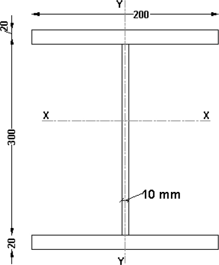
Design – column lacing – illustration 6.9
As per Euler’s formula, the critical load for the column is determined by the expression

For this section, the distribution of material is such that the moment of inertia about the XX axis is obviously greater than the moment of inertia about the YY axis.
The value of moment of inertia about YY,
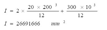
With the constrained defined, the effective length of the column shall remain equal to its actual length.
Hence, Leff = 3000 mm
Therefore, critical load,
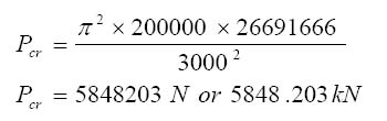
Therefore, the safe load-carrying capacity of the column is 5848.2 kN.
Illustration 6.10: Two channel sections, back-to-back, have been used to withstand a compressive load of 1100 kN. The overall arrangement of this section, along with sectional properties, is shown in Figure 6.27. The objective now is to design a lacing system for the built-up section. The value of yield stress for the steel is 250 N/mm.
We now undertake the design of lacing fastened with rivets. As the back-to-back distance for the channels is 22 cm and the rivet line is at 5 cm from the back of the channel, the horizontal distance between the fasteners would be 35 cm.
As the first step, the lacing member would be kept at 45° with the horizontal. Also, the fastening with the main member is through a single rivet. In this case,
Effective length of the lacing bar l = 32×√2 = 45.3 cm
Spacing between the lacing bars L = 2 × 32 × tan 45° = 64 cm
We know that for the independent channel sections, rmin = 2.8 mm. Also, the overall slenderness ratio for the built-up section is 4.5.8.
Hence, 50× rmin = 50 × 2.8 = 140.
And 0.7× Maximum Slenderness Ratio × rmin = 0.7×45.8×2.8 = 89.76.
Since L is less than both of these values, it is acceptable to adopt.

Design – column lacing – illustration 6.10
The next step would be to determine the appropriate section for the lacing bar.
For this, we know that the minimum thickness of a lacing bar in single lacing should not be less than l/40. In this case,
l/40 = 45.3 /40 = 1.13 cm.
Hence, the design would adopt the flat, with a 12 mm thickness. Since the battens would be fastened with rivets, we take the width of the trial section as 65 mm.
Hence, the slenderness ratio for batten plate = leff×√12 / t = 45.3×√12 / 1.2 = 130.77.
Since the value of the slenderness ratio is less than 145, this section can be adopted. Also, for the slenderness ratio of 130.76, the permissible direct compressive stress for steel (yield stress = 250 N/mm2) obtained from the table is about 56.6 N/mm2.
The column is subjected to direct compressive load of 1100 kN. As per the design requirement, the lacing member should withstand a shear force equivalent to 2.5% of the direct load.
Transverse shear force on lacing = 2.5% × 1100 = 27.5 kN.
Since lacing is being provided on both the faces of the built-up section, the corresponding bars on both faces would share the load equally.
Hence, shear for one lacing face, T = 27.5 / 2 sin 45 = 13.75 kN.
The direct force induced in the lacing bar due to this shear force,
F = T/sin 45º = 13.75/sin 45º = 19.45 kN.
Each lacing member would be subjected to direct tensile or compressive force of this magnitude. Let’s check if the section of the lacing bars is adequate for it.
Net compressive stress = 19.45×1000 / 12×65 = 24.93 N/mm2.
This is less than the observed maximum permissible value of 56.6 N/mm2.
If the member is fastened with 20 mm nominal diameter rivets,
Net tensile stress = 19.45×1000 / 12×(65–21.5) = 37.26 N/mm2.
In this case too, the actual stress is much less than the maximum allowed stress of 60% of the yield value. The design can safely be adopted.
Splicing in columns
Rolled steel sections come in standard lengths and it is not always possible to obtain the desired length. In some situations, the section of column itself may undergo a change at a particular location. In all such situations, it becomes necessary at times to join the separate pieces of rolled section. The method of joining those pieces with the help of additional plates is known as splicing.
Splice plates are designed to transmit all the forces that are in existence at the joint. It includes direct compression as well as the bending moment and shear force, if present. It is clear that if the sectional areas of the plates for web and flanges were at least equal to the original area of the individual web or flange, they would serve their purpose. The further design process involves determination of total load on each splice and accordingly decides the fastening for the splice plates.
The following example explains the design process of column splicing.
Illustration 6.11: An I-section of 200 mm depth and 125 mm flange width has a compressive load of 350 kN acting axially. In addition, there is moment acting at the splice section of 10 kNM.
Since the section under consideration is symmetrical about both X and Y axes, the splice system would also be symmetrical about these axes. In other words, the size and location of both the flange plates would be similar. The same applies to the web plates.
Total axial load = 350 kN.
Load on each splice = 350/2 = 175 kN.
The moment at the splice plate would add to the load on the splice. The magnitude of the load due to moment would be equal to
Moment / Section Depth = 10 / (200/1000) = 50 kN.
This load due to moment would be tensile for one splice and compressive for the other. Since we require both the plates to be similar, we would design them for the worst combination of loads.
The largest magnitude of load on each splice = 175 + 50 = 225 kN.
The average thickness of flange and web are 14 mm and 9 mm respectively. Hence, 16 mm thick and 200 mm wide plates on each of the flange would serve the purpose. For the web, a plate of 8 mm thickness on both the sides of the web has been provided.
Design of fasteners
It has been decided to provide fastening with 20 mm nominal diameter rivets. For these rivets,
Allowable stress in shear = 90 N/mm2
Allowable stress in bearing = 270 N/mm2
Strength of rivet in single shear = π/4 ×(21.5) 2 × 90 = 32674 N = 32.67 kN
Strength of rivet in bearing = 21.5 × 14 × 270 = 81270 N = 81.27 kN
Therefore the rivet value is 32.67 kN.
Number of rivets required for each splice,
N = 225/32.67 = 6.88
Hence each flange plate shall be provided with eight rivets on both sides of the joint.
The rivet arrangement is shown in Figure 6.28.

Column splice- design details – illustration 6.11
6.9 Design of beams
Beams are structural members, normally with their axes horizontal, which are subjected to loads normal to their longitudinal axis. Beams eventually transfer these loads to one or more of the supports it has. Due to the nature of loading a beam is subjected to bending moment and shear force over its span.
Classifications of beams
In the case of a grid of beams, those beams that transfer the load directly to the vertical structural members, i.e., columns and walls, are termed as main beams. The beams, which directly support the floor construction and in turn are supported on main beams, are termed as secondary beams. Main beams receive the load from secondary beams. The term joist is used for beams made of light structural sections. A heavy-sectioned major beam in a structure is known as a girder. In the case of excessively heavy loads, which may be encountered in industrial structures, bridges, etc., it is common practice to form a suitable section by fastening plates of different sections together.
Such beams are known as plate girders. The photograph of such a plate girder is shown in Figure 6.29.

Plate girder with stiffeners
Beams are also classified, based on the function they perform. In the case of sheds made of columns and roof trusses, horizontal beams spanning two adjacent trusses are known as purlins. Those beams that rest on the purlins are known as rafters. In the case of buildings, the beams that span doors, windows and other openings in the walls and support the masonry above these openings are known as lintels. The beams provided along the peripheral wall of a building, that support part of the floor, as well as the wall up to the floor above, are known as spandrel beams. The beams that support the stairs are called stringers.
Besides, based on the supporting systems, beams are classified as simply supported, cantilever, fixed, continuous, etc.
Beams of varying strength
As we studied in the previous section, the extreme fibre faces the maximum amount of stress in the beams. To make the beam economical, the strength in extreme fibre is designed to bear the maximum stress, while the central fibres, where the stress is less, are designed accordingly. This is the reason that most of the beams are made up of “I”- or “C”-shaped channels.
Rolled steel sections and their behavior under lateral loading
We are already familiar with rolled steel sections and their various shapes available. Among the rolled steel sections, I-sections, channel sections, tee sections, etc., are the regular sections, which are most commonly used as beams. In all these sections, most of the material is located near the top and bottom faces, i.e., in the flanges as compared to the web portion. Such rolled steel sections provide a large moment of inertia about the X axis. As a result, these sections provide a larger moment of resistance as compared to solid rectangular, square and circular sections of the same cross-sectional area. These sections, as such, are considered most efficient and economical. In the case of I-sections, the large flange width of these sections provides greater lateral stability. The web-flange construction of the section also facilitates easy connection with other structural members. Channel sections have reasonably good lateral strength but poor lateral stability. They are also unsymmetrical about the Y axis and are subjected to unsymmetrical bending on loading. Angle sections and tee sections are used as beams for light loads. There sections are weak in resisting bending.
In most situations, beams are loaded in the direction perpendicular to the X axis. This is done to ensure that the bending of beams occurs about X axis, the moment of inertia of the section about which is actually the largest. Very rarely is the application of load allowed in the direction perpendicular to the Y axis.
In the case of loading the beam, the application is considered to be through the shear centre of the beam sections. The shear centre for the beam section is the centroid of the sectional area. Such load application ensures that the loading produces just plain bending about either one or both of the axes. In such cases, the section is subjected to simple bending and shear. When the load does not pass through the shear center, a torsional moment is produced in addition, along with the bending moment, which attempts to twist the section. It becomes imperative then to design the sections by considering stresses induced by torsion, in addition to normal flexural and shear stresses. Sections like angles and channels are prone to inducement of torsional stresses. For such sections, a special load device may be used so that the load passes through the shear center of the section and the torsional moment may be avoided.

Castellated and open web beam sections
A number of times the sectional properties of a rolled steel section are enhanced by cutting the beam in a pre-determined pattern along the web and then rejoining both the separated parts in a fresh pattern. This way, the section modulus of the beam increases, without any increase in the weight of the beam. These sections are known as castellated or open web sections. The reason for calling them ‘open web’ is that cutting and rejoining of the web leaves a number of similar and regular openings in the web. Examples of a few such sections are shown in Figure 6.30 and a photograph in Figure 6.31. Castellated sections are economical for light loading conditions.
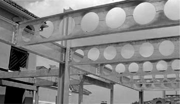
Photograph -open web beam
Moment resisting properties of the section
Here, it would be pertinent to recall the important expression pertaining to bending moment, the derivation of which was observed in Chapter 3. The expression has been

Here, M is the value of bending moment at a section, I is the moment of inertia of the section, y is the distance of fibre from the neutral axis and f is the magnitude of stress in the fibre.
Or M = f × (I/y).
The above equation holds well when the plane of bending coincides with the plane of symmetry of the beam section. The bending of the beam occurs in the principal plane of the beam section. In this expression, it is possible to treat any component as variable. However, while undertaking the actual design of a beam, normally the construction material is frozen beforehand based on a number of factors. Along with it, the value of f also gets decided, though there always remains some degree of flexibility regarding the ultimate grade of the construction material.
The magnitude of maximum bending moment (M) in the beam is a function of structural geometry and the loading system. Hence, it is also known at the time of actual determination of the beam section. The self-load of the beam is factored in the dead load of the structure at the beginning of the analysis. A small variation in it will not alter the design results in any significant way.
The last component of the expression is I/y. Though constituted of two elements, it is reasonable to treat it as one. The reason is that both I and y are functions of the size and shape of the cross section. As is clear from the expression, other thing being constant, the moment-carrying capacity of a beam is directly proportional to the moment of inertia of the section and inversely proportional to the distance of the outermost fibre from a neutral axis. This expression, I/y, is termed as the section modulus and denoted with Z. In most beam design problems, the objective is to provide a section with the required value of Z in combination with the lowest possible value of sectional area.
Mathematically stated, Z ≥ M/(ftan or ften).
When the section of beam is symmetrical about the neutral axis, the value of y is equal to half the depth of the section. In addition, the maximum bending stress in compression and in the tension at the extreme fibres would be equal. In case the beam section is not symmetrical about the neutral axis, then the distances of extreme compression fibre and extreme tension fibre, from the neutral axis, would be different.
As shown in Figure 6.32, if y1 and y2 are the distances of two extreme fibres from the neutral axis, the values of extreme bending stresses would be different. It is also to be ensured that maximum bending stress in the beam section is less than the allowable bending stresses, whether tensile or compressive. The stress triangles for the section above and below the neutral axis are shown in the diagram. For the state of equilibrium at the section, the total compressive force ‘C’ above the neutral axis would be equal to the tensile force ‘T’. These two forces act in opposite directions and form a couple. The arm of the couple is equal to the distance between the centroids of the two stress triangles.

Distribution of bending stress along beam cross-section
This couple resists the bending moment due to external loads and, therefore, its magnitude is known as the moment of resistance (Mr):
Mr = (C × Arm ‘L’) or (T × Arm ‘L’)
6.9.1 Beam design process
We do by now understand the theoretical aspects of beam design. Now we observe the process through which a design is actually undertaken and the factors that influence the process.
Determination of section – permissible stresses in tension and compression
In the first step, the minimum required section modulus is determined from the relationship between maximum bending moment and permissible stress values. Once the value of Z is known, the appropriate section is decided by adopting a section with a value of Z nearest to the required value.
It may be noted here that the permissible bending stress for steel in tension and compression is a function of its yield stress. As mild-carbon steel exhibits similar properties in tension and compression, the permissible values for both stresses can be taken as follows:
Permissible bending stress, σbt or σbc = (2 / 3)×fy or 0.66×fy
However, there is another factor affecting the value of permissible bending stress in compression. We know that when a beam is subjected to positive bending moment, its portion above the neutral axis is subjected to compression and the portion below the neutral axis is subjected to tension (in the case of negative bending moment, the nature of stresses would obviously be opposite). The magnitude of stress in a fibre is proportional to its distance from the neutral axis.
Let us examine the effect of this phenomenon on the rolled beam section. These sections are so developed that the flanges remain at the maximum distance from the neutral axis. Consequently, they are subjected to the largest stresses. The top flange is subjected to compressive load and the bottom flange is subjected to tensile load, both of large orders. If we visualize the top flange independent of the section, it is equivalent to a compression member with low moment of inertia about one of its axis. If not restrained laterally, the flange would have a tendency to buckle like any compression member. As a result, it becomes necessary to link the value of allowable stresses in the compression flange with the slenderness ratio and the degree of restraint imposed.
As per the norms, if the compression flange connectivity is such that due to structural fastening or friction a lateral load equivalent to 2.5% of the total force in the flange can be resisted, the beam would be classified as restrained and normal bending compressive stress would be permitted. Otherwise, the beam would be termed as unrestrained and the permissible stress would be derived fresh with the aid of various formulae and stress tables provided in design codes.
Checking for shear
Once the section is decided, it is necessary that it should be checked for its adequacy against shear stress. We already know that the shear stress in a beam section varies across the section and the maximum value of shear stress is 1.5 times the average value. In the case of flange web sections, the shear-carrying capacity of a flange is ignored due to the complex distribution of stress in it.
If the maximum value of shear force at any section along the beam is V, overall depth of the beam is D and the thickness of the web is tw, the average value of shear stress for the section would be determined by the following expression:
Shear Stress, τcal = V / (D × tw)
The maximum permissible value for shear stress is normally limited to 0.45×fy.
Checking for web crippling
The section is further checked for web crippling. As shown in Figure 6.33, the web may cripple locally due to the effect of concentrated load. The potential spot for this is the location where the flange joins with the web. As shown in the diagram, the load is supposed to disperse at an angle of 30º. If the magnitude of load/reaction is W, the width of bearing for load is a and the depth of the critical section is hf, the value of bearing stress at the section would be
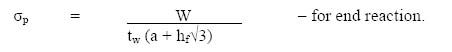

Beam design – web crippling
And 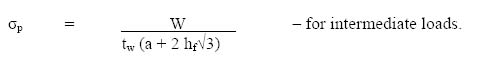
The maximum permissible value of σp is normally not allowed to exceed 0.75×fy.
Checking for web buckling
Besides the potential of failure in bearing, the web may buckle under the influence of a concentrated load. This again is a local phenomenon. The load is supposed to disperse at an angle of 45º. The effective web length for this purpose is taken at the level of the neutral axis. If W is the magnitude of load/reaction, hw is the clear height of web between the flanges and B is the effective web length offering resistance, the value of direct compressive stress in the web would be as follows:

The value of σc thus calculated should be less than the permissible compressive stress for a member with the slenderness ratio hw√3 / tw.
In case this condition fails to get fulfilled, it would be necessary to provide stiffeners below the location of concentrated load.
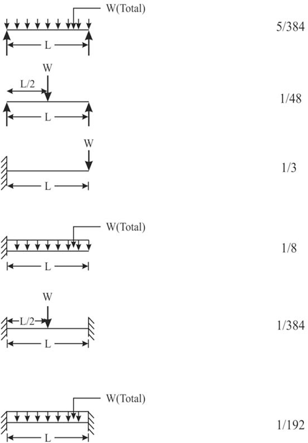
Deflection in beams – values of ‘K’
Checking for deflection
The maximum permissible deflection in a beam is normally expressed in terms of the span of the beam. As per general norms, it should not exceed 1/325 of the total span, though there can be higher deflections permitted in certain cases. Since deflection is a functional aspect, a certain degree of flexibility is allowed based on the material of construction and finishing, which are being supported.
The expression for maximum deflection in any beam is as follows:

Here all the values, except K, are quite familiar. K is the constant, which depends on the load configuration and supporting arrangement for the beam. The values of K for different conditions are given in Figure 6.34.
The following illustration further explains the steps involved in the beam design process.
Illustration 6.12: A steel beam of 6 m span is resting on 250 mm thick brick walls at both its ends. The beam has been made of a 450 mm deep I-section. Both the flanges have been further strengthened with flange plates of 16 mm × 200 mm section. We are now required to determine the maximum amount of uniformly distributed load, which can be allowed on the beam, if the compression flange is laterally restrained. The yield stress for steel can be taken as 250 N/mm2.
The sectional properties for a 450 mm deep I-section are as follows:
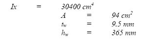
First of all, we determine the permissible bending stress in tension and compression. Since the compression flange is effectively restrained,
Permissible value of bending stresses = 0.66 × fy =0.66 × 250 = 165 N/mm2.
The next step would be to determine the moment of inertia of the composite section. Since the composite section is also symmetrical about the X axis of rolled section, the neutral axis for the composite section would continue to remain the same. The arrangement is shown in Figure 6.35.
The moment of inertia of the combined section with respect to the X axis,
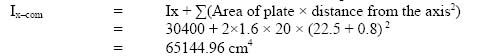
The value of section modulus for this section,
Z = Ix–com / (d/2) = 65144.96 / (22.5 + 1.6) = 2703.1 cm3
The maximum moment carrying capacity of the section,
M = Z × σbc or σbt (σbc and σbt do have similar values in this case)
Hence, M = 2703.1 × 165 × 100 = 44601150 N-cm = 44601 kN–cm.
Since the beam is simply supported with a clear span of 4 m and an end bearing of 250 mm, the effective span would be equal to the center-to-center distance between the supports.
Effective Span ‘L’ = 6 + 0.125 + 0.125 = 6.25 m.

Beam design – stress distribution
In the structural terms, the beam is a simply supported one. If the amount of uniformly distributed load on the beam is w kN/m, the maximum bending moment (at mid span) shall be expressed by the following equation:
Mmax = w×L2/8
Equating it to the maximum load-carrying capacity of the section,
44601 = w× 100 ×(6.25 × 100)2/8.
Hence, w = 91.3 kN.
From the parameter of flexural stress, the beam can be subjected to a UDL of 91.3 kN/M. Here, for the sake of simplicity, we are ignoring the self-weight of the beam.
However, it is still required to check the section against shear, deflection and web buckling.
Check for shear
The total load on the beam ‘W’ = 91.3 × 6 = 547.8 kN.
Maximum Shear Force = Support Reaction (R)= W/2 = 547.8/2 = 273.9 kN.
To resist this shear force, only the web area would be considered.
Maximum Shear Stress = Maximum Shear Force / (D × tw)
= 273.9×1000 / (450 × 9.5)
= 64.1 N/mm2
The maximum allowed shear stress is equivalent to 0.45 times the yield stress. In this case, it is 112.5 N/mm2. Since the actual shear stress (64.1 N/mm2) is lower than this value, the section is safe in shear.
Check for deflection
In the case of a simply supported beam subjected to UDL, the amount of maximum deflection is given by the following expression:
Maximum Deflection = 5 × W×L3
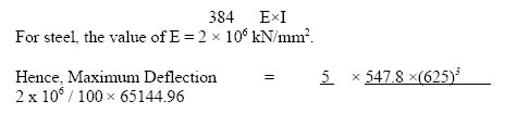
The actual deflection of 1.33 cm is less than this value. Hence, the loading on the beam is acceptable, based on deflection parameters.
Check for web crippling
Since the load on the beam is uniformly distributed, the potential spots for web crippling are the supports only.
The expression for bearing stress is
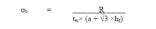
Here, hf = Depth of root of the fillet from flange top = 37.5 mm for the section
A = Width of bearing at the support = 250 mm for the case
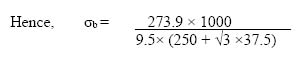
= 91.54 N/mm2
The maximum allowed bearing stress is equivalent to 0.75 times the yield stress, which is 187.5 N/mm2 in this case. However the actual bearing stress (91.54 N/mm2) is lower than this value. Hence, the section is not prone to web crippling at the supports.
Check for web buckling
For reasons similar to the case of web crippling, the potential location for web buckling would be the supports. The reaction force at the supports would be considered dispersing at 45°. The location to check the stress is at the centre of the web.
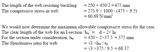
For this slenderness ratio, the value of permissible compressive stress is 134.5 N/mm2. This is far in excess of the actual direct compressive stress and, therefore, the section is safe from web buckling.
As all the checks indicate that the section is safe enough to withstand the calculated uniformly distributed load, the capacity of beam to withstand a UDL of 91.3 kN/M, inclusive of self-weight has been established.
6.10 Design of truss and allied structures
Trusses are the multiple member structures, the analysis of which we already have learnt in the previous chapters. Trusses are used to support roofs, decks of bridges, etc. Such applications are shown in the photographs in Figure 6.36 and Figure 6.37, respectively.

Trussed shed with allied structures

Trussed bridge
In this section, we would restrict our attention to the roof trusses and allied structures. Trusses are economical over beams in the case of large spans and are therefore provided for large columnless areas. At both the ends, trusses either rest on columns or on walls. As we have seen, while understanding the analysis of the truss, all the loads are supposed to act on the nodes of the truss. The structural arrangement is planned to facilitate this. The roof covering is supported on beams, termed purlins, which span between the trusses. The longitudinal axis of purlins is at right angles to the axis of the truss. These purlins transfer the load from the roof (dead load and wind load) upon the trusses. The top rafters of the trusses are also tied with rafter bracings. The ends of the building are known as gable ends, which may or may not be provided with the truss.

Trussed building – components
A general arrangement of the trussed building (plan) is shown in Figure 6.38.
Design of truss members
As we already know, truss members are only subjected to direct forces, either compressive or tensile. Though there can be exceptions, the members are not allowed to be subjected to bending and shear force. Hence, once the analysis for the truss has been conducted and the load for each member is known, further process is only to design the section of these tension or compression members, as per the procedure applicable.
Since the design of truss involves the analysis of forces in its members and determination of appropriate sections, for these members, which already has been explained in the earlier part of this manual, we will not repeat the same. At the same time, certain important points related to truss design have been described below:
- The pitch of the truss (its height to span ratio) is maintained in the range of 1/4 to 1/6.
- The purlins, with their axis inclined with respect to the vertical, would be subjected to bending about both its axes.
Trusses may be subjected to either moving load if they are supporting a bridge deck, or wind load, if they are supporting a roof. Due to the dynamic nature of these loads, the magnitude of induced forces in individual members keeps varying. In fact, they can even change in nature from tensile to compressive and vice versa. Hence each of the members is designed for the highest force it can subject to, with due consideration to possible reversal of forces.
While designing the rafter bracing, the stiffness provided by purlins is totally ignored.
6.11 Conclusion
In this chapter, we obtained familiarity with the design process, which is a logical progression from the exercise of structural analysis.
Also in this chapter, we have studied the behavior and characteristics of steel, which are important from the point of view of its use as a structural material. Its deformation under loading, which is of prime importance, has been studied in detail.
We have also understood design principles and procedures of fasteners, tension and compression members and beams. These are the basic elements of any structural system, and understanding of their design can make one appreciate the entire design process, which would be undertaken in the design of large and complex structures.
This chapter has ended with an introduction to trusses and allied structures. The trusses are very important structures for covering any kind of span; it is very important for an engineer to understand them.
This chapter will enable the reader to understand the behavior of reinforced cement concrete as a composite structural material. The reader will also be able to understand the design process of various types of structures made of this material, using the previously understood principles of structural analysis and design.
Learning objectives
After completion of this chapter, one will be able to:
- Fully understand the behavior of concrete as a structural material and the factors that influence this behavior
- Understand the principles of design of this composite material
- Understand design techniques, based on working stress theory, used in a number of structures commonly constructed with reinforced cement concrete
- Obtain a reasonable degree of familiarity with the principles of pre-stressed concrete construction
Reinforced Cement Concrete (RCC) is undoubtedly the most widely used construction material. It is, perhaps, the most versatile of all construction materials. The advantages of using RCC for construction are manifold. It can be produced at any location, can be designed to adopt the locally available constituents for its production and gives great flexibility regarding component size and shape to the designer and constructor. Besides, concrete is a well-researched material and its properties are quite well understood.
7.1 Concrete – the material
Concrete is a word of Latin origin. It refers to a material that hardens under water. In construction practice, concrete is a mix of cement, aggregate, water and occasional admixtures, which remains plastic at the time of manufacturing. Subsequently, as a result of chemical action between cement and water, the mixture loses its plasticity and gains strength.
The process of losing plasticity (termed setting) is quite rapid and takes from a few minutes to few hours, depending on various factors. The process of gaining strength (termed hardening) is a prolonged one and continues for a very long period after the setting of the concrete. These properties of concrete, and the associated property of not being prone to any chemical reaction by water in the later periods of its life, are very important and have contributed to the widespread use of concrete as a building material.
The relationship between the constituents of a concrete mix can be described in more than one way. It is possible to view hardened cement as the main component of formation and aggregate as the filler or diluter. Another way to look at it is by viewing the aggregate as the main structural component, something like masonry, bonded together by cement. Research and analysis has established that if one tries to use cement alone as a construction material, the disadvantages are aplenty. Cement has certain negative characteristics such as excessive shrinkage, creep, heat generation during hydration, etc., which are brought down in magnitude due to the presence of aggregate. Hence, aggregate in concrete has a role larger than that of mere filler. At the same time, aggregate can hardly be considered as the main component in concrete. Therefore, it is sensible to view concrete as a material consisting of two phases: the hydrated cement phase and the aggregate phase. The overall properties of concrete are dependent on the combination of the properties of these two.
After referring to concrete as a two-phase material, now we will discuss its characteristics further with special reference to the modulus of elasticity of the composite product. We know that the value of modulus of elasticity is one of the most important aspects for structural design. Concrete, being a composite material, cannot be assumed to have a constant value. Due to the two-phased structure, concrete can be viewed to have two possible forms, which are fundamentally different from each other. The first is of an ideal composite hard material, which has a continuous matrix of an elastic phase with a high modulus of elasticity and embedded particles of a lower modulus. The second possible form can be that of an ideal composite soft material, which consists of elastic particles with a high modulus of elasticity, embedded in a continuous matrix phase with a lower modulus. The difference between the calculated modulus of elasticity in both the cases can be large. In the case of a composite hard material, it is assumed that the strain is constant over any cross section while the stresses in the phases are proportional to their respective moduli. While in the case of composite soft material, the modulus of elasticity is based on the assumption that the stress is constant over any cross section and the strain in the phases is inversely proportional to their respective moduli. For practical purposes, a fairly good approximation is derived based on assumptions for composite soft material for mixes made with normal aggregates.
We will now observe the properties and contribution of each ingredient of the concrete. As stated earlier, concrete has the following ingredients:
- Cement
- Aggregate (large and small)
- Water
- Admixtures
7.1.1 Cement
A product with binding characteristics is called cement. For concrete, the most commonly used cement is Portland cement. Portland cement is the name given to cement obtained by intimately mixing together calcareous and argillaceous materials, alumina, and iron oxide-bearing materials; burning them at a high temperature (called clinkering temperature) and finally grinding the resulting clinker. Normally no material other than gypsum, water and grinding aids may be added after burning.
From the description of Portland cement given above, it can be seen that it is made primarily from a combination of a calcareous material, such as limestone or chalk, and of silica and alumina found as clay. The manufacturing process, described briefly below, consists of grinding the raw materials into a very fine powder, mixing them intimately in predetermined proportions and then burning the mix in a large rotary kiln at a temperature of about 1350 °C. In the kiln, the material fuses partially and forms a clinker. The clinker is cooled and ground to a fine powder with some gypsum added to produce commercial Portland cement.
A typical composition limit for Portland cement is shown in the table below:
| Ingredient | Content in Percentage |
| CaO | 60 – 68 |
| SiO2 | 17 –24 |
| AI2O3 | 3 – 10 |
| Fe203 | 1 – 6 |
| MgO | 0.1 – 4 |
| Sulphates | 1 – 3 |
| K2O, Na2O | 0.2 – 1.5 |
| Others | 1 |
The mixing and grinding of the raw materials can be performed either in water or in a dry condition and the process classifications, wet and dry, arrive from here. The mixture is fed into a rotary kiln, which can be as large as 7 m in diameter and 225 m in length. The longitudinal axis of the kiln remains slightly inclined. The mixture is fed at the upper end, while pulverized coal is blown in by an air blast at the lower end of the kiln. As the mixture of raw materials moves down the kiln, it encounters a progressively higher temperature so that various chemical changes take place along the kiln. First, water, if any, is driven off and CO2 is liberated from calcium carbonate. Further on, the dry material undergoes a series of chemical reactions and in the hottest part of the kiln about 30 percent of the material turns liquid. All the raw materials—lime, silica and alumina—recombine at this stage. The mass then converts into balls of 3 to 25 mm diameter, known as clinkers. These clinkers are cooled through heat exchangers. The cool clinkers, which are very hard, are ground with gypsum to avoid flash or very rapid setting of the cement during hydration.
Chemistry of cement
We have seen that the raw materials used in the manufacture of Portland cement consist mainly of lime, silica, alumina and iron oxide. In the kiln, these compounds react with each other to form a series of more complex products and a state of chemical equilibrium is reached. However, equilibrium is not maintained during cooling, and the rate of cooling will affect the degree of crystallization and the amount of amorphous material present in the cooled clinker. Nevertheless, cement can be considered as being in frozen equilibrium, i.e., the cooled products are assumed to reproduce the equilibrium.
Four compounds are regarded as the major constituents of cement. They have been listed in the table below:
| Compound | Chemical Composition | Notation |
|---|---|---|
| Tricalcium silicate | 3CaO.Si02 | C3S |
| Dicalcium silicate | 2CaO.Si02 | C2S |
| Tricalcium aluminate | 3CaO.Al203 | C3A |
| Tetracalcium aluminoferrite | 4CaO.Al2O3.Fe203 | C4AF |
The silicates, C3S and C2S, are the most important compounds. These are responsible for the strength of the hydrated cement paste. In reality, the silicates in cement are not pure compounds but contain minor oxides. These oxides have significant effects on the atomic arrangements, crystal form and hydraulic properties of the silicates.
The presence of C3A in cement is undesirable as it contributes little or nothing to the strength of cement, except at the early stage of hydration. However, C3A is beneficial in the manufacture of cement since it facilitates the combination of lime and silica.
C4AF’s presence in cement is small in proportion and its effect on the cement characteristics is relatively insignificant. However, it reacts with gypsum to form calcium sulphoferrite and its presence may accelerate the hydration of silicates.
The amount of gypsum added to the clinker is crucial and depends upon the C3A content and the alkali content of cement. Increasing the fineness of cement has the effect of increasing the quantity of C3A available at early ages, which raises the gypsum requirement. An excess of gypsum however leads to expansion and consequent disruption of the set cement paste. The optimum gypsum content is determined on the basis of the overall generation of the heat of hydration so that a desirable rate of early reaction occurs. This ensures that there is little C3A available for reaction after all the gypsum has combined.
In addition to the main compounds described, there are minor compounds such as MgO, TiO2, Na2O, K2O, Mn2O3, etc. They usually do not exceed a very small percentage of the mass of cement. Two of the minor compounds, the oxides of sodium and potassium (Na2O and K2O), are termed as alkalis. They have been found to react with some aggregates. The products of the alkali aggregate reaction can cause disintegration of concrete. This reaction also affects the rate of the gain of strength of cement. We, therefore, should understand that the use of the term minor refers primarily to the quantity of the compounds and not necessarily to their importance.
Hydration of cement
The process of chemical reaction of cement with water is known as hydration. Till now, we have discussed the properties of cement, but the material of actual interest to a structural engineer in practice is the set cement paste. This is the product of the reaction of cement with water. In the presence of water, the silicates and aluminates of Portland cement form hydrates. These produce the hardened cement paste in the course of time. As stated earlier, the two calcium silicates (C2S and C3S) are the main cementitious compounds, with the former hydrating much more rapidly than the latter. In normal cement, the calcium silicates contain small impurities from some of the oxides present in the clinker. These can have a strong effect on the properties of the hydrated silicates. The product of hydration of C3S is the microcrystalline hydrate, with some lime separating out as crystalline Ca (OH) 2. C2S behaves similarly though it takes less lime. The reaction of pure C3S with water is very rapid and would lead to a flash set, which is prevented by the addition of gypsum to the cement clinker. Even so, the rate of reaction of C3S is quicker than that of the calcium silicates.
The chemical reaction involved in the hydration of cement is exothermic. The resultant heat generated is known as the heat of hydration and is expressed per gram of cement. The temperature at which hydration occurs has a bearing on the amount of heat produced. In normal Portland cement, about one-half of the total heat is liberated between the first and third day and about three-quarters of the total heat is liberated in the first seven days of reaction.
Types of cement
There are various types of cement that differ in properties, like setting time, strength, etc. Some of them are used only under adverse situations. The common types of cement have been described below:
- Portland pozzolana cement – The term Pozzolana is used for a siliceous material which possesses little or no cementitious properties, but in the presence of water it reacts with calcium hydroxide (liberated during the hydration of cement) to form compounds possessing cementitious properties. The commonly used pozzolanas in the manufacture of this type of cement are burnt clay, shale or fly ash. The proportion of Pozzolana in cement may vary from 10% to 25% of the overall weight. Portland Pozzolana cement produces lower heat of hydration and has greater resistance to attack of chemical agencies than ordinary Portland cement.
- Portland blast furnace slag cement – In this case, the normal cement clinkers are mixed with up to 65% of blast furnace slag for the final grinding. The resulting cement is quite cheap and has almost the same characteristics as Portland cement. In its early stage, the strength development remains slower than that of normal cement but the eventual strength remains the same. In addition, it offers very high resistance to dilute acids. In view of its having a low heat of hydration and better resistance to chemicals, this cement can be used in mass concrete works such as dams, heavy foundations, retaining walls, etc., as well as for the construction within a sea.
- High alumina cement – This cement is manufactured by using 40% each of bauxite and lime, 15% of iron oxide and 5% of silica, magnesia, etc., as raw materials and grinding the clinkers to a very fine powder. High alumina cement has an initial setting time of about three to four hours. Once set, it hardens quite rapidly and the 24 hours compressive strength becomes as high as can be obtained from other types of cement after a minimum period of seven days. It also has excellent resistance to action of sulphates.
- Rapid hardening cement – Rapid hardening cement attains high strength at an early stage. The property of high early strength is achieved due to a high degree of fineness, burning at relatively high temperature and high lime content. The strength development of this cement at the age of three days and seven days is almost the same as the respective seven days and 28 days strength of ordinary Portland cement with the same water cement ratio. The main advantage of using rapid hardening cement is that the formwork/moulds for the members can be removed faster.
- Low heat cement – In the case of mass concrete work such as dams, massive retaining walls, etc., the rate of loss of heat from the surface is much lower than the buildup of heat of hydration inside the concrete mass. This results in setting up tensile stresses during curing and finally leads to cracking of concrete. In low heat Portland cement, the amounts of tri-calcium aluminate and tri-calcium silicate, which contribute the maximum towards heat generation, are kept to the minimum.
- Quick setting cement – If concrete is to be laid under water, quick setting cement is used. The setting action of such a cement starts within five minutes and it becomes stone hard in less than an hour. Quick setting cement is mixed with a small percentage of aluminum sulphate and is ground much finer than ordinary Portland cement.
- White cement – White-colored cement is useful for terrazzo flooring, face plaster to walls and other ornamental works. It is also used for putting markings on grey cement surfaces like roads or airstrips. To manufacture white cement, the raw materials used are china clay and pure limestone while completely excluding iron oxide. For burning the rotary kiln, oil is used as fuel instead of coal. The strength of white cement is less than that of ordinary cement.
- Sulphate-resisting cement – This type of cement is used in the construction of foundations in soils where the sub-soil water contains a very high proportion of sulphates. The constituents of sulphate-resisting Portland cement are such adjusted that the tri-calcium aluminate (C3A) and tetra calcium aluminate-ferrite (C4AF) remain very small. Cement with such composition has excellent resistance to sulphate attack.
7.1.2 Aggregates
Aggregates are materials bonded by the cement paste in concrete. Aggregates are largely viewed as inert, inexpensive materials dispersed throughout the cement paste so as to produce a large volume of concrete. But strictly speaking, aggregates are not truly inert because their physical, thermal and chemical characteristics influence the performance of concrete. From the economic viewpoint, it is advantageous to use a mix with as much aggregate and as little cement as possible. The cost benefit has off course to be balanced against the desired properties of concrete in its fresh and hardened state. As aggregate form one of the phases of the two-phased composition of concrete, the properties of aggregate directly affect the properties of the concrete. The aggregate for a concrete mix should be hard, strong, dense, durable and free from foreign materials like clay, loam, vegetable and other injurious matter. The presence of these deleterious substances prevents proper adhesion of cement, on the surface of aggregates, and thus adversely affects the properties of the concrete.
Aggregates are derived from natural rocks or alternatively manufactured from products like slag, etc. Natural aggregates are formed by the process of weathering and abrasion or by crushing of a larger parent mass.
Many properties of the aggregate depend on the properties of the parent material, which include chemical and mineral composition, specific gravity, hardness, strength, pore structure, colour, etc. In addition, there are certain properties of the aggregate, which are not dependent on the parent rock. These are particle shape and size, surface texture, etc. All of these properties do have a considerable influence on the quality of fresh or hardened concrete.
Even in the case if all the aggregate properties are known, it is not quite easy to define a good aggregate for concrete. While aggregate with satisfactory properties would make good concrete, aggregates, which seem to have some drawback, may also produce good concrete. For instance, a material in rock form may disrupt on freezing but may not do so when embedded in concrete in aggregate form. In general though, aggregate performing poorly under one or more than one criteria is unlikely to make satisfactory concrete.
Size and origin of aggregates
Concrete is made with aggregate particles, covering a range of sizes with maximum particle size normally between 10 mm and 75 mm, the selection depending on a host of factors. Particle size of about 20 mm for aggregate is widely adopted for concrete production. At times, low-strength concretes are made with a single aggregate containing all the sizes and known as all in aggregate. However, good-quality concretes are always produced with multiple aggregate sizes, termed as fine and course. The size limit of 5 mm divides the fine aggregate (also called sand, if obtained naturally) from coarse aggregate. Fine aggregates or sand, normally, have a lower size limit of about 0.075 mm (75 μ) or a little less. Material with particle size between 0.0 6mm and 0.02 mm is classified as silt and still smaller particles are termed as clay.
Fine aggregate – As stated earlier, the material below 5 mm in size is termed as fine aggregate. Natural sand or crushed stone dust is mostly used in concrete mix. Sand used from any source, when used in a concrete mix, needs to be properly tested to ensure that the total percentage of clay, silt, salts and other such organic matter does not exceed specified limits. Sand grains may be round or angular. Angular grained sand has good interlocking property that results in a strong mortar. Sea sand should not be used in its natural state for RCC work, as the chloride salts present in the seawater are liable to attack the steel reinforcement.
Coarse aggregate – The material with particle size in excess of 5 mm is termed as coarse aggregate. The size of the coarse aggregate used depends upon the nature of work, size of the component, density of reinforcement, etc. The maximum size may be up to 200 mm for mass concrete applications such as dams. Crushed hard stone and gravel are the most common materials used as coarse aggregates for structural concrete. Clinker slag and coke breeze are also used as aggregates for lightweight and insulating concrete where strength requirement is not really high.

Coarse aggregate
The photograph of a typical coarse aggregate is shown in Figure 7.1.
Grading of aggregates
To produce concrete of a desired strength, density, durability and imperviousness, the proportion of all its ingredients has to be such that the cement paste is sufficient to fill the voids in the fine aggregates and the mortar thus produced is sufficient to fill the voids in the coarse aggregates. To fulfill this objective, the fine as well as the coarse aggregate is graded suitably. It means that the proportion of different particle sizes is so maintained that the smaller particles fill the voids between the larger particles to the maximum extent. This results in a low percentage of voids in the mix. The reduction in percentage of voids results in a corresponding reduction in the quantity of mortar required to fill the voids of the coarse aggregates and, consequently, there is a reduction in the quantity of cement required to make the concrete. Thus, grading of aggregates is necessary to effect economy in the production of concrete.
The grading limits for aggregates are maintained as per the provision of relevant concrete mix design codes. The codes provide tables and graphs for the purpose, applicable for all categories of aggregate.
7.1.3 Water
Water is another important ingredient of concrete. Water chemically reacts with cement and the resultant hydration produces the gel of requisite bonding characteristics. Therefore, it is not possible to produce concrete without water.
The water for concreting should meet the following norms:
- It should be free from oils, fats, etc.
- It should be free from injurious amounts of acids or alkalis.
- It should be free from iron content, organic matter and any other substance, that is likely to have an adverse effect on concrete or reinforcement.
- It should be fit for drinking purposes
The functions of water in the concrete mix can be described as below:
- It acts chemically with cement to form the binding paste for the aggregates as well as the steel reinforcement.
- It acts as a lubricant for the aggregates in the mix and facilitates proper mixing.
- It provides moisture to the aggregate in order to prevent them from absorbing water that is vital for chemical action.
As true for any chemical process, a minimum quantity of water is essential to accomplish the complete hydration process. This is expressed in terms of percentage weight of cement and the range varies from 20% to 25%, depending on the type of cement. However, the fact is that if the water proportion in the mix were maintained just enough to complete the hydration, the mix would hardly be workable and would have low moulding ability. Hence, for a well-prepared plastic concrete, the requirement of water is higher than that derived from chemical consideration.
Water–cement ratio
The ratio of the weight of water to the weight of cement within a concrete mix is known as the water–cement ratio for that mix. Research has established that for a given proportion of ingredients in a concrete mix, there is almost a fixed amount of water (optimum, which gives maximum strength). A small variation from the optimum quantity of water causes a large variation in the strength of concrete. If the amount of water used is less than the optimum quantity, the resultant concrete will be difficult to place in the formwork and can pose problems in compaction. It is difficult to ensure complete setting of the cement in these circumstances and the strength of concrete gets reduced appreciably. On the other hand, if the quantity of water used is more than optimum, the result would be the formation of excessive voids in the hardened concrete, which can reduce the strength and density of the concrete and can also affect its durability. Thus, the water–cement ratio serves as a yardstick for obtaining concrete of the desired strength. The lower the ratio, the greater would be the strength of the mix. Since the water requirement for chemical action is much lower than the one required for workability of the concrete, the water proportion in a concrete mix can always be brought down with appreciation in its other properties. A mix rich in cement would thus have a lower water–-cement ratio and, therefore, higher strength compared to a mix lean in cement.
7.1.4 Admixtures
Admixtures in the concrete are external compounds, which are added to concrete in order to enhance one or more of the physical properties of the concrete. The addition of admixtures is purely optional in the manufacturing of concrete. At times, it is possible to change some of the properties of more commonly used cement types by incorporating a suitable additive or an admixture. In other cases, such addition of admixtures serves the sole purpose of achieving the desired effect. A large number of products are available in the market with their desirable effects described. But such products may also have some undesirable effects, so a cautious approach is warranted while using the admixtures. In normal practice, the terms ‘additive’ and ‘admixture’ are used interchangeably, although, strictly speaking, additive refers to a substance added at the cement manufacturing stage, while admixture is added at the mixing stage.
In most cases, the admixture acts chemically with the cement to produce the desired result. The examples of chemical admixtures are plasticizers, retarders and accelerators. In addition, there are compounds like air-entraining agents whose main purpose is to protect concrete from the deleterious effects of freezing and thawing.
Accelerators
Accelerators are generally referred as those admixtures that accelerate the process of development of the early strength of the concrete. The strength accelerator may not affect the setting time but necessarily influences the hardening pattern of the concrete. It may be worth mentioning here that quick-setting admixtures also exist, which specifically reduce the setting time. Sodium carbonate is one example of a quick-setting admixture that promotes a flash set in the cement.
Retarders
Retarders are those admixtures, which delay the setting of concrete. In other words, retarders increase the setting time for cement. Retarders are useful when concrete is being poured in hot weather and higher temperature reduces the setting time. Sugar is one of the most common examples of retarder. Apart from this, carbohydrate derivatives, such as soluble zinc salts, etc., are the others in this category. When used in a carefully controlled manner, about 0.05 per cent of sugar by mass of cement will delay the setting time by about 4 hours.
The use of retarding admixtures slows down the development of the early strength of concrete, but the rate of strength development goes up later, so the ultimate strength development remains practically unaltered. Retarders also tend to increase the plastic shrinkage because the plastic stage is extended, but the drying shrinkage remains unaffected.
Plasticizers
Plasticizers are essentially water-reducing admixtures. In concrete, these are used to achieve the following objectives:
- To increase the workability of the mix, so as to ease its placement in hard to access locations.
- To achieve a higher strength by decreasing the water/cement ratio at the same workability as an admixture-free mix.
The principal active components of water-reducing admixtures are surface-active agents, which are concentrated at the interface between two immiscible phases and which alter the physico-chemical forces at this interface. With the influence of admixtures, water freed from the system becomes available to lubricate the mix, so that its workability goes up. The reduction in the quantity of mixing water, which is possible owing to the use of admixtures, varies between 5 percent and 15 percent. A part of this reduction is, in many cases, due to the entrained air introduced by the admixture. The actual decrease in mixing water depends on the cement content, aggregate type and the air-entraining agent, if present. Trial mixes are therefore essential to achieve optimum properties as well as to ascertain any potential undesirable side effects like segregation, bleeding and loss of workability with time.

Shuttering for wall concreting and concreted walls
The plasticity of wet concrete is a very important characteristic, especially when the structural member is slender or the concentration of reinforcement within it is high. This can be appreciated by observing the case of concrete wall construction, the shuttering of which prior to concrete pouring and its finish post concreting are shown in Figure 7.2.
7.1.5 Properties of concrete
The most important properties of concrete are the following:
- Strength
- Durability
- Workability
Strength of concrete – Strength is the most important property of concrete. The hardened concrete must be strong enough to withstand all the imposed stresses, taking into account the factor of safety. Factors like strength of the cement, water–cement ratio, aggregate properties, etc. have basic influence on the strength of concrete. Proper placement, compaction and curing are the other factors governing the strength of concrete. Curing is important to supplement the moisture to the green concrete, the loss of which can retard the process of hydration.
The strength of the concrete is measured by the crushing test on the cubical or cylindrical specimen of it. As is obvious, the test provides the compressive strength of the concrete. All other types of strength for concrete are the function of its compressive strength. The structural design of concrete members is based on the characteristic compressive strength of a 15 cm cube specimen of age of 28 days. It is, however, important to note that the process of hydration of cement in concrete continues even after 28 days and, consequently, concrete continues to harden with age, although at a slower rate.
The strength of concrete is expressed in the form of its 28-day characteristic strength. ‘28 days’ indicates the age of the concrete. The age is worked out from the instant when water is mixed with other ingredients, cement and aggregates of the concrete. The characteristic strength of concrete is the value of compressive stress at which not more than 5% of the specimens are expected to fail. In other words, 95% or more specimens of the concrete are certain to attain that strength.
A factor of safety is applied to the strength of concrete, the value of which depends on the nature of stress and circumstances of use. In the case of bending compression, a factor of safety of 3 is normally used. A higher factor of safety is adopted for the direct compressive force.
Durability of concrete – Durability is that property of concrete by virtue of which it resists the process of disintegration and decay. Disintegration of concrete may be the result of:
- Use of unsound cement or less durable aggregates, coarse or fine, in the preparation of concrete.
- Its exposure to harmful chemicals.
- Freezing and thawing of water within it, sucked through the cracks by capillary action.
- Expansion and contraction resulting from temperature changes.
The resistance of concrete to chemical attack, weathering, etc., to a very large extent, depends upon the conditions of exposure, grade of concrete used, quality of its materials and the extent of voids and pores present in the concrete mass. The magnitude of cover provided over reinforcement and the degree of imperviousness of a concrete mix also influence the durability of the concrete. Concrete can be made durable:
- By using good-quality materials.
- By using adequate quantity of cement.
- By maintaining a low water–cement ratio.
- By reducing the extent of voids by suitable mix design.
- By adequate compaction and curing of the concrete.

Measurement of slump to check concrete workability
Workability of concrete – Workability is the property of wet concrete due to which the concrete can easily be mixed, transported, placed in formworks and compacted. Despite its importance, workability is a somewhat elusive property of concrete and is difficult to define and measure. A workable concrete mix must be fluid enough so that it can be compacted with the minimum labor. A workable concrete does not result in bleeding of slurry or segregation of aggregate from the mix.
The Slump Test measures the workability of freshly prepared concrete, where concrete is poured into a container of the shape of frustum of a cone. The cone is removed post compaction and the slump is measured. This is indicated in the photograph in Figure 7.3.
Placement, compaction and curing of concrete
For best results, concrete should be placed and compacted immediately after mixing. The arrangement for the conveyance of the concrete mix should be so planned that the mixed mass is used before its initial set, which normally is a period between thirty to sixty minutes. Hence, it should be possible to place the quantity of concrete prepared in one batch within this period. In order to prevent the shuttering from absorbing the water from the concrete or getting stuck to it, a coat of oil or grease is usually applied to it (the shuttering).

Concrete Mixer
The fresh concrete is prepared by mixing all the ingredients either in a portable mixer (photograph of shown in Figure 7.4) or in large capacity batching plants (shown in Figure 7.5).

Concrete batching plant
While placing this freshly prepared concrete, it should be laid in layers 100 to 300 mm thick based on the shape and size of the overall component, with each layer properly compacted before laying the next one. Compaction of concrete should proceed immediately after placing. The function of concrete compaction is to expel the air bubbles in the mass and make it impermeable enough to attain the desired strength. Compaction is normally done by the use of mechanical vibrators. The resultant concrete is more impermeable, dense and free from honeycombing. The process of concrete placement around reinforcement and its compaction by vibrators is shown in Figure 7.6.

Concrete pouring and compaction
Curing of concrete is one of the essential requirements after placement. Curing is the process of keeping the set concrete continuously damp for some days, in order to enable the concrete to gain more strength. It has been established that the strength of concrete increases with age provided it is kept moist. The period for which curing should be continued depends upon atmospheric conditions, such as temperature, humidity and wind velocity. In general, the process of curing should be continued for seven to 10 days. In cold weather, however, the concrete ought to be cured for longer, as the rate of hardening of cement is low. Efficient curing increases both impermeability and durability of the concrete. Both covering the exposed surface with moist cloth and sprinkling water at intervals to keep the covering wet or by impounding water within bunds over the entire flat area may do curing. The alternate process of curing with steam enables the concrete to gain the required strength in lesser time.
7.2 Principle of reinforced concrete design
As we know by now, concrete is a heterogeneous conglomerate of cement gel and aggregates. Though extremely strong in compression, due to its intrinsic structure, concrete is quite weak in tension. Its resistance to tension is so low that plain concrete can be used only when the member is subjected to pure compression and no bending at all. On the other hand, steel has equal strength in compression and tension. But while a long steel member or bar can develop its full strength in tension, it cannot resist an equal amount of compressive force due to its tendency to buckle. Also, a pure steel structure can be very expensive, as well as ugly. Therefore, if the combination of concrete and steel is used in such a way that both materials are subjected to the stresses they are most able to withstand, it would amount to their optimum utilization in the structure. Reinforced Cement Concrete (RCC) is designed on the same principle.
The RCC is a composite material of construction. The combination of steel and concrete is effective and workable due the following reasons:
- The bond between concrete and steel is quite effective. Concrete grips the steel tightly while setting and hardening. Therefore, the transmission of force from concrete to the steel bars becomes possible and easy.
- The co-efficient of linear expansion, for concrete and steel, is almost the same. Therefore, no internal stresses develop within reinforced concrete structures due to variations in temperature.
- Both materials are not chemically reactive with each other. The coating of cement grout on the surface of steel bars protects them from corrosion and does not produce any adverse chemical effect.
7.2.1 Advantages of reinforced concrete
RCC has the following main advantages when compared with other alternatives like steel:
- RCC normally proves more cost-effective compared to steel.
- Different components of the structure are cast monolithically, which gives high rigidity to the structure.
- Concrete is durable, fire resisting and free form corrosion. These properties get extended to the RCC also.
- Concrete, and therefore RCC, is almost impermeable to moisture.
- The flexibility of reinforcement and the plastic properties of concrete make the moulding of reinforced concrete members in any desired shape possible. Hence, structures of any size and sectional shapes can be constructed with the RCC.
7.2.2 Reinforcement and its bond with concrete
For RCC construction, concrete is reinforced with steel and this material acts as a composite one. Since there can be no fastening to join the two materials, their composite behavior is completely dependent on the development of the bond between the two.
The bondage strength between steel and concrete depends upon the two factors:
- Concrete quality
- Surface characteristics of steel
The quality of concrete, measured as strength and denseness, contributes to its capacity to hold the steel firmly. The more the strength and compactness of concrete, the more will be the strength in bonding. As the strength of the bond depends upon the surface of steel also, the bondage will be better if the steel bar has small ribs on its surface. Such steel is termed as deformed steel. Design codes provide the values of the bond strength, which normally range from 0.6 N/mm2 to 1.2 N/mm2 for concrete with a characteristic strength from 15 N/mm2 to 40 N/mm2. The bond strength is normally increased for deformed bars by a factor of 1.4.
When a reinforcement bar is embedded within the concrete, the effort to pull it out would certainly be met with some resistance. This resistance would be equal to the permissible bond stress for the combination of steel and concrete, multiplied by the surface area on which it is working. If the reinforcement steel is of circular section of diameter d and the permissible bond stress is τb, the resistance force would be
= τb ×π×d×L
Here, L is the length of embedment of steel. The above expression gives the value of the force required to break the bondage. It is obvious that the steel bar would be imposed to this much force before it comes out of concrete.
If the length of embedment is increased gradually, a stage will arrive when the tensile strength in the steel would equal to its limiting value. If the permissible tensile strength for steel were σs, the tensile force in the bar would be as follows:
T = π×d2×σs,
At this stage, the load developed in the bar is the ultimate allowed and the length of embedment required is known as the development length of reinforcement for its full strength. If the length were Ld, the bond strength developed would be equal to
= τb ×π×d×Ld
Equating both the expressions above,

Hence, 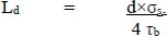 .
.
The above relationship informs about the minimum length of reinforcement required beyond the section to develop appropriate amount of strength in it. It may be noted that we did consider the pulling out of reinforcement in the case, which induces tensile strength in the bar. If instead of the pulling out a rod we try pushing it within the concrete, it can be visualized that the resistance will be higher. Hence for compression, the development length can be calculated by considering 25% higher value of bond stress.
In the compression,  .
.
7.2.3 Theory of RCC section design
To design an RCC structural section, the following assumptions are made:
- A transverse section, which is plane before bending, remains plain after bending.
- The modulus of elasticity of steel and concrete are constant and not stress dependent.
- All tensile stresses are taken up by the steel reinforcement only and the tensile load on concrete is nil.
- The bond between concrete and steel is sufficient to make them act jointly to resist tensile or compressive forces. No slippage takes place between the two materials.
For any composite material, the relationship between the modulus of elasticity of its components is extremely important. This is helpful in deriving the distribution of the load between its components. In the case of RCC section design, the ratio between the modulus of elasticity of steel and concrete is known as the modular ratio and is denoted by m. Hence, if Es and Ec are the modulus of elasticity for steel and concrete respectively, the modular ratio can be described as
m = Es / Ec
Now, we would derive the actual distribution of the load. As per assumptions made above, it is evident that if a beam were subjected to bending that causes compression at the top face and tension at the bottom, the strain in the steel and concrete would be equal at the interface where both meet.
For steel,
Strain = σst / Es
And for concrete,
Strain = σcbc / Ec
where
σst = Tensile stress in steel
σcbc = Compressive stress in concrete
Since both the strains are equal,
σst / Es = σcbc / Ec
σst / σcbc = Es / Ec
σst / σcbc = m
σst = σcbc × m
Therefore, the stress in the steel would be m times the value of the stress in the surrounding concrete.
In the next step, we need to determine the overall stress bearing capacity of an RCC section. For this, consider the section shown in Figure 7.7. The overall area of the section is A, with the area of concrete and steel being Ac and At respectively. If the permissible compressive stress in steel and concrete were σsc and σcc respectively, the overall capacity of the section to withstand the compressive load would be

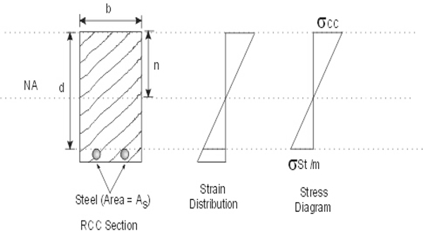
RCC section and stress distribution

We know that Ac + At = A. Hence,

The above is the relationship between the total compressive force and the compressive stress in the concrete. The expression ‘A + At(m – 1)’ is termed as the equivalent area of the section, represented in the form of concrete area.
During bending, the transverse section, which is plane before bending, remains plane after bending. It is, therefore, obvious that when bending takes place in a beam, the strain in any layer remains proportional to its distance from the neutral axis. Thus, the strain diagram will be a straight-line diagram as shown in Figure 7.7. Also drawn is the stress diagram. Since it is assumed that the overall section is transformed into equivalent concrete section, it becomes essential to write the stress in steel in terms of equivalent stress in concrete at the level of steel. In the stress diagram, the stress in steel is replaced by equivalent stress in the concrete surrounding the steel.
Unlike steel sections, the location of the neutral axis in the RCC beam of given dimensions is not fixed and varies with the amount of steel provided in the section. We will observe the reason for it. It is clear from Figure 7.7 that the section of the beam above the neutral axis is subjected to compression, while that below the neutral axis is subjected to tension. As is assumed that no tensile force is resisted by concrete, the whole of the tension below the neutral axis is supposed to be resisted by the steel reinforcement. Thus, the effective depth of the beam would be equal to the distance measured from the top face of the beam to the center of the tensile reinforcement.
We will consider the case of a singly reinforced section shown in Figure 7.7. In the singly reinforced section, the steel bars are provided to resist only the tensile force and the concrete resists the entire compression. Assuming that for the case the steel and concrete have been stressed to their ultimate permissible values, the neutral axis of a beam can be determined as below.
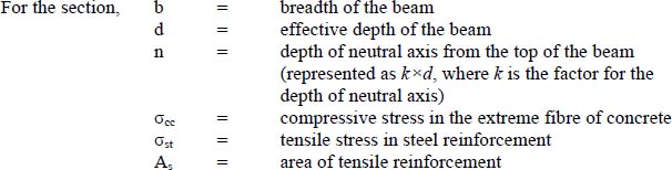
Referring to the stress diagram in Figure 7.7,

From this,

If we represent the stress ratio σst/σcc as r, the expression would become

The above expression gives the location of the neutral axis for a reinforced concrete section. It may be noted here that both concrete and steel have been assumed to be stressed to their highest permissible limits. Such a section is known as the balanced section and the value of k would be dependent on the stress ratio and the modular ratio.
Next, we would determine the capacity of the balanced section to withstand moment. In the case of RCC section, the size or diameter of steel reinforcement is quite small compared to the overall size of the section. The variation of bending stress along this small dimension would be quite small. Hence, the tensile stress in the steel is assumed to be uniform over the total area of tensile steel and is considered to act at the centre of the steel. For the purposes of deriving design expressions, the rectangular section of the beam is treated to consist of a block of concrete above the neutral axis for resisting the whole of the compression force and the area of steel below the neutral axis is assumed to resist all the tensile forces. The concrete below neutral axis is completely ignored as far as resisting the load is concerned.
Total compressive force in the concrete above neutral axis = b×k×d×(σcc /2)
Total tensile force in the steel below neutral axis = As × σst
As is evident from the stress diagram, the compressive force would act at a distance of n/3 or k×d/3 from the top edge of the section. The tensile force would work at the bottommost edge of the section.
For a section to be in equilibrium, both the above forces should be equal in magnitude:

It is obvious that these forces would form a couple. The length of arm of the couple would be equal to (d – n/3).
Hence, moment of resistance of the section,

The lever arm (d – n/3) can be expressed as equivalent to j×d, where j is known as the lever arm factor:

Using this value of j in the expression for the moment resistance of the section,
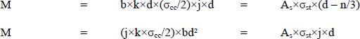
Here again, the expression (j×k×ςcc/2) is denoted as R, the moment of resistance factor.

From the above relationships, for a particular value of moment, the requirement of sectional size as well as steel area for a balanced singly reinforced RCC section can be determined.
Under and over reinforced RCC sections
The RCC section where the area of steel provided is less than that required as per the above-derived expression is known as the under reinforced section. In this case, the steel being deficient in quantity it attains the maximum stress value ahead of concrete and the concrete, in turn, never reaches its maximum stress value. In such cases, the location of the neutral axis remains above the neutral axis for the balanced section, as shown in Figure 7.8.
For the under reinforced section, the moment of resistance is derived by the relation
M = As×σst×(d – n/3)

Stress distribution in over and under reinforced sections
The RCC section where the area of steel provided is larger than that required as per the expression valid for the balanced section, the section is known as the over reinforced section. In this case, the concrete attains its maximum stress value ahead of steel. In this situation, steel never reaches its maximum stress value. In such cases, the location of the neutral axis remains below the neutral axis for the balanced section, as shown in Figure 7.8
For the under reinforced section, the moment of resistance is derived by the relation
M = b×k×d×(σcc/2)×(d – n/3)
Process for design of singly reinforced section
The objective of design of a moment resistant section in RCC is to derive the most economical sectional size for the given value of moment. Accordingly, the area of steel required is calculated.
Since the values of permissible stresses and modular ratio are known, the first step would be to calculate the value of k from the relevant formula. With this known, the lever arm factor j can be derived.
Next would be the derivation of the moment of resistance factor, R, with the formula given below:
R = j×k×σcc/2
The moment of resistance of the section is the function of R and the width as well as the depth of the section. Since the size of the section has to be determined yet, we move ahead by assuming a suitable width for the section. With the help of this, the required depth of the section can be determined by using the formula
M = Rbd2
As a final step, the area of steel reinforcement can be determined by the expression

The illustration below would explain the procedure more clearly.
Illustration 7.1: An RCC beam is subjected to bending moment of 150000 N-m, with the moment due to self-load factored in. It is desirable to determine a section for it. Since the wall size right below the beam is 250 mm, it is desirable to restrict the beam width to 250 mm only.
The allowable stresses are as follows:

First of all, we need to determine the value of k for the section. Using expression,
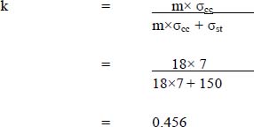
Moment arm factor,

For the section, the value of coefficient of the resisting moment,
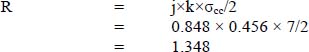
We know that the moment of resistance of the section,
M = Rbd2
The value of M is known and the value of R for the case has been derived. Also, the width b of the section has been restricted to 250 mm. By placing these values into the expression above,

The effective depth of the beam should be 667.2 mm. Giving consideration to the cover for the bottom reinforcement, the overall depth of 700 mm can be provided.
With the section being designed as balanced, the area of steel required would be derived from the following expression:

To fulfill this requirement, four steel bars of 25 mm diameter each (total area = 1963 mm2) can be provided as reinforcement.
Design of doubly reinforced RCC sections
In the previous section, we have studied the design principles and procedure for singly reinforced RCC sections. It may be noted here that the singly reinforced RCC beams of given dimensions have a limiting value of moment which it can resist. To enhance this value what is required is to alter the composition or grade of its components. This may not be feasible or economical at times.
Also while analyzing continuous beams and frames, we have seen that the sign of the bending moments can be different for different portions of a beam. It may be positive at the centre of the span but can turn negative over the supports. This means that the tension generation may be at different faces within a single span of the beam.
In situations as above, designing a doubly reinforced section may be a solution. In doubly reinforced beams, steel is provided in tension as well as in the compression zone. Unlike singly reinforced sections, steel bears both tensile and compressive loads in a doubly reinforced section. Since the compressive reinforcement is restrained from all sides by the concrete, there is no scope for compression reinforcement to buckle and, therefore, the value of permissible stress is independent of the slenderness of the steel bars.
When subjected to compressive stress, concrete undergoes elastic deformation. Apart from this, when concrete is consistently subjected to compressive loads, it undergoes a slow plastic deformation, also known as the creep. Therefore, for the same amount of stress, the deformation of concrete is more in the case of compression in comparison to tension. As a result, the modulus of elasticity for concrete is more in tension and somewhat lower in compression. In other words, the modular ratio for compression would be higher in the case of a doubly reinforced section. If the modular ratio in tension is m, a corresponding value of 1.5m is adopted for compression. In view of this, the equivalent area of steel in compression would be equivalent to

The stress diagram for a doubly reinforced section is similar to a singly reinforced section. Hence, the following relationship, for the location of neutral axis, would be valid in the case of a doubly reinforced section also:

As was in the case of a singly reinforced section, the above expression gives the location of neutral axis for the balanced section. If the actual neutral axis does not coincide with it, the exact location of the neutral axis can be derived by taking moment of all the forces on the section with respect to the neutral axis.
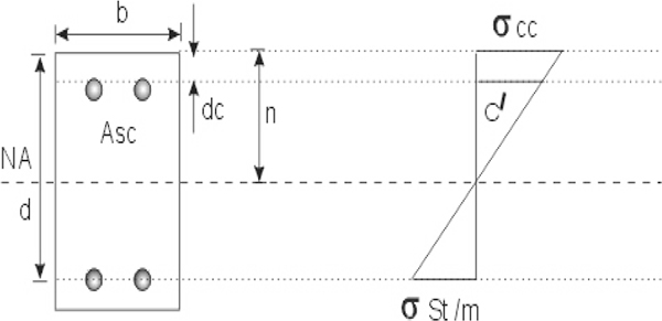
Stress distribution in doubly reinforced sections
Referring to Figure 7.9, by equating the moment of compressive force with that of tensile force, we will have
bn2 / 2 + (mc– 1)×Asc×(n – dc) = m×Ast×(d – n)
The moment of resistance of a doubly reinforced beam would be equal to two components. First is the moment of resistance, ignoring the compressive reinforcement and treating the beam as singly reinforced (M1). The other one would be the moment of compressive force in the steel reinforcement, with the distance between the center of tensile and compressive reinforcement as the lever arm (M2). The total moment of resistance would be equal to the sum of the two.
Hence, M = M1 + M2.
We already know the expression for the moment of resistance, for a singly reinforced section, and the procedure to derive the area of reinforcement. Here, we would see the expression for moment due to compressive reinforcement. Again referring to Figure 7.9 and taking moment about the centre of the tensile reinforcement,

To balance the compressive reinforcement, there would be need of additional reinforcement in the tensile zone. Its area can be calculated from the following expression:
Ast2 = M2/ ςst× (d – dc)
Shear stress treatment in RCC section
We understand that in a beam section, the bending moment is generally accompanied with shear force. This is due to the fact that load and support systems, which induce bending moment, are also conducive to the generation of shear force.
If a concrete section, with width b and depth d, is subjected to shear force V, the value of shear stress in the section should be equal to
τ = V / b×d
We also know that the shear stress distribution along the section is not uniform but parabolic. Hence, the above expression gives only the average shear stress on the section. The maximum value of shear stress would be along the neutral axis and also be equal to 1.5 times the average value.

RCC section – shear stress distribution
In the case of RCC sections, the treatment of distribution of shear stress is still further different from a pure concrete section. In the case of RCC sections, the concrete in the tensile zone is neglected and the shear force is assumed to be resisted by the bond between steel and concrete. The distribution of the shear stress across the section is shown in Figure 7.10.
The area of the shear force diagram in this case is the sum of the area of the parabolic portion above neutral axis and the rectangular portion below neutral axis.
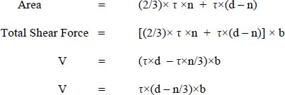
We know that (d – n/3) is equal to the lever arm, j×d.

When the shear stress acts on an RCC section, as shown in Figure 7.11, a set of complementary stresses develops in a plane perpendicular to the shear force. The resultants of these do act along the diagonal of the block under shear force. As is obvious from the diagram, the force along one diagonal plane would be tensile and compressive along other.

Complementary shear stress
Due to the development of these forces, there would be a tendency of either crushing of the material along one diagonal or the rupture of the material along the other. The actual failure would be dependent on the tensile and compressive strength of the material, as the lower value of the two would govern the type of failure. We know that concrete has a much lower strength in tension than in compression. Hence, the concrete section would tend to split along the diagonal representing tensile force.
When a concrete section is subjected to shear force, it resists a certain amount of it due to a combination of frictional resistance in the compression zone (tension zone is ignored as concrete has a tendency to separate here) and the vertical component of the aggregate interlock force. In the RCC section, the shear force across the reinforcement adds to this resistance. Hence, a certain amount of shear stress can safely be allowed to develop in the RCC section, the value of which is decided on the basis of the characteristic strength of the concrete in combination with the percentage area of reinforcement in the overall RCC section. If the actual shear stress exceeds this value, shear reinforcement is provided in the shape of vertical stirrups. However, it may be noted that the value of shear stress in a section, for a particular grade of concrete, is never allowed to exceed the values provided in the design code. If the value of shear stress is found to be more than this value, the section itself is required to be redesigned. These stirrups act as direct tension members and prevent the separation of concrete along the plane of shear failure.
For these vertical stirrups, the design shear force is taken as the difference between the total shear force at the section and the shear resistance of the section. If a section has width b and depth d, the designs shear force Vd shall be derived by the following expression:
Vd = V – τp×b×d
Here, τp is the permissible shear stress for the section.

Shear stirrups
The vertical stirrups are made of plain steel bars of diameter ranging from 5 mm to 12 mm. The stirrups can be single or multi-legged, depending upon the shear force they are required to resist. The typical shapes of the stirrups are shown in Figure 7.12. They are either anchored with the compression reinforcement or taken around both the tension and compression reinforcement to form a closed loop.
While designing a stirrup system, the diameter and number of legs are decided by judgment and based on these, the spacing between these stirrups is derived.
We would refer back to Figure 7.10, where the elevation of a beam near its support has been shown. We know that for a simply supported beam, the amount of shear force becomes largest at the supports. Hence, the area around support would be prone to the maximum shear stress. The shear crack development is at the 45º to the axis of the beam; hence, longitudinally, it would extend to the distance equal to beam depth from the edge of the support.
If, d = Effective depth of the beam
σst = Permissible tensile stress in the stirrup
As = Cross-sectional area of the stirrup
s = Spacing of the stirrups
then
Tensile force resistance capacity of each stirrup = As × σst
Within the critical longitudinal length of d, the number of stirrups would be equal to d/s.
Hence, tensile force resistance capacity of all stirrups 
This tensile force bearing capacity has to be equal to or more than the value of shear force Vd, derived earlier.


This expression gives the design value of stirrup spacing in the design of vertical shear stirrups.
By now, we are quite familiar with the characteristics of concrete and design of RCC as a composite material. Let us examine the application of this knowledge in the design of some structures.
7.3 Design norms for reinforced concrete beams
We already have gained sufficient knowledge about the beam as a structural member. Beams are predominantly subjected to bending and shear forces. The fundamentals of the analysis of beams and design of an RCC section are well understood by now. Therefore, the design of RCC beams should not be a difficult task.
At the same time, the process of design can become easier if the following norms are followed in the analysis and design stages.
7.3.1 Effective span
Simply supported beam – The effective span of a simply supported beam or slab is taken as the distance between the center-to-center of support or the clear distance between the supports, plus the effective depth of the beam, whichever is smaller.
Continuous beam – In the case of a continuous beam or slab where the width of the support is less than 1/12 of the clear span, the effective span shall be calculated as in the case of a simply supported beam.
In case the supports are wider than 1/12 of the clear span or 600 mm, whichever is less, the effective span shall be calculated as below:
- For end span with one end fixed and the other continuous or for intermediate spans, the effective span shall be the clear span between supports.
- For end span with one end free and the other continuous, the effective span shall be equal to the clear span plus half the effective depth of the beam or slab or the clear span plus half the width of the discontinuous support, whichever is less.
Beams part of frames – In the analysis of a continuous beam, which is part of a frame, the effective span shall be taken as the center-to-center distance between the supports.
Depth of beams from the viewpoint of deflection
It is necessary to impose a limit on the magnitude of deflection in a structural member with a view to ensure that the extent of deflection does not adversely affect the appearance or efficiency of the structure. Also, the structural behavior of the material may be different from the assumed one if the deformation is excessive. We can theoretically calculate the deflection for a specified case of loading on the structure. However, till 10 M span of the beam, the requirement related to deflection is very likely to be met if span to depth ratios for different beams are within the following limits:
- For Simply Supported Beam – 20
- For Cantilever Beam / Overhang – 7
- For Continuous Beams – 26
Proportioning against slenderness
As in the case of steel beams, the compression zone of the RCC beam would also have a tendency to buckle. The required stability is maintained, by proportioning the cross section of the beam. For non-cantilever beams, the clear distance between the lateral supports does not exceed 60b or 250b2/d, whichever is less. Here, d is the effective depth of the RCC section and b is the breadth of the compression face of the beam, with a location at the middle of the supports. In the case of cantilever beams, the clear distance from the free end to the lateral restraint should not exceed 25b or 100 b2/, whichever is less.
Limits related to reinforcement steel
For an RCC section, the provision of reinforcement steel is governed by certain norms, which ensure optimum performance.
Some of these norms are as follows:
Tension reinforcement
- The minimum area of the tension reinforcement in beams shall not be less than that derived by the following expression:As / bd = 0.35 / fy
Here, As is the area of steel as tensile reinforcement and fy is the yield strength of the steel.
- The maximum area of tension reinforcement in a beam should not exceed 0.04 bD, where D is the overall depth of the beam.
Compression reinforcement
There has been no lower limit for compression reinforcement, as it can very well remain absent in the section. However, the maximum area of compression reinforcement in a beam shall not exceed 0.04 bD, where D is the overall depth of the beam.
Curtailment of reinforcement
It is known that the value of bending moment varies across the length of the beam. Reinforcement in a beam section is decided according to the highest value of the bending moment, and, therefore, some of it can become redundant at sections away from the high moment locations. In view of this, the main reinforcement in beams and slabs may be discontinued or curtailed at the location where it is no longer required to resist bending. However, it is necessary that the curtailed reinforcement should extend beyond the section for a distance equal to the effective depth of the member or 12 times the bar diameter, whichever is greater.
Side face reinforcement
Where the depth of the RCC beam exceeds 750 mm, it becomes necessary to provide side-face reinforcement along both the faces of the beam. The total area of such reinforcement shall be not less than 0.1 per cent of the sectional area of beam web and they shall be distributed equally on the two faces, at a spacing not exceeding 300 mm or web thickness, whichever is lower.
Shear reinforcement
In RCC beams, minimum shear reinforcement in the form of stirrups should be provided as derived by using the following expression, irrespective of the requirement as per stress level:

The maximum spacing of shear reinforcement along the axis of the beam should be maintained as 0.75d or 450 mm, whichever is less.
Concrete cover to reinforcement
The thickness of the concrete portion between the outermost edge of reinforcement steel and the outermost edge of the concrete section is known as the clear cover for the reinforcement. The clear cover of concrete to reinforcement in different structural members should be as follows:
- The clear cover of longitudinal reinforcing bar in a beam should not be less than 25 mm or the diameter of the reinforcing bar, whichever is higher.
- The clear cover at the each end of reinforcing bar in a beam should be equal to or more than 25 mm or twice the diameter of such bar, whichever is higher.
- If the surface of concrete of a structural member is exposed to the action of harmful chemicals, acids, saline atmosphere, etc., or is in direct contact with soil containing such chemicals, it is suggested to provide additional cover ranging from 15 mm to 50 mm over and above the normal cover.
- For reinforced concrete members permanently or periodically immersed in seawater, the cover of concrete should be 50 mm more than the normal cover.
Spacing of reinforcement
The gap between the reinforcements in RCC sections is governed by factors like diameter of the bars, aggregate size of the concrete, etc. The norms for spacing of reinforcement are within the section are as follows:
- The minimum clear gap between two parallel main reinforcing bars should not be less than the diameter of the bar (or the diameter of the larger bar, if unequal) or 5 mm more than the nominal maximum size of coarse aggregate used in the concrete, whichever is more.
- If main reinforcement bars are provided in two or more layers one over the other, the minimum clear gap between any two layers of the bars should normally be the largest of the three,
- 15 mm,
- two-thirds the nominal maximum size of aggregate, or
- the maximum size of the bar.
The following illustration would make clear how these provisions are followed in the design exercise.
Illustration 7.2: A simply supported RCC beam is subjected to a live load of 13500 N/m, apart from its self-weight. The beam is supported on columns of 250 mm × 250 mm section. The clear span for the beam is 4.5 m. The objective is to design an appropriate section.

To design a section, we need to determine the highest bending moment within the span of the beam. Since the sectional size of the beam is not known, we assume an overall section of 250 mm × 400 mm for it to determine the bending moment. Since the values of 60b and 250d2/b both are much higher than the clear span of 4 m, the section meets the safety norms related to slenderness.
For each meter length of beam, the self-weight would be

Total load on beam = Live Load + Self-Load

Since the center-to-center distance in the beam (4.5 + 0.25 = 4.75 m) is less than the sum of the clear span and beam depth (4.5 + 0.4 = 4.9 m), 4.9 m would be considered as the span for the beam.

Now, from the data about material characteristics, we will determine the value of k for the section. Using expression,
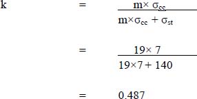
Moment arm factor,

For the section, the value of coefficient of the resisting moment,

We know that the moment of resistance of the section,

The value of M is known and the value of R for the case has been derived. Also, the width b of the section has been kept 250 mm, according to the width of the supporting columns. By substituting these values into the above expression,

The effective depth of the beam should be 372.4 mm. We have assumed an overall depth of 400 mm, which should be fine giving consideration to the clear cover requirement of 25 mm for the main tensile reinforcement.
As we are designing a balanced section, the area of steel required would be derived from the following:

To provide reinforcement as per this requirement, four steel bars of 20 mm diameter each (total area = 1256 mm2) are proposed.

This is very close to the minimum norm of 25 mm, and, hence, is acceptable.
Check for minimum area requirement for tension reinforcement
The minimum area for tension reinforcement can be calculated from the following expression:

Since the area of actual steel provided is much higher (1256 mm2), the section meets the relevant norm completely.
Design of shear reinforcement
We know that the maximum shear force would be at either one of the supports.

For this percentage of steel and concrete with characteristic strength of 20 N/mm2, the permissible value of shear stress in the section is 0.435 N/mm2.
Hence, the shear force withstanding capacity of the section = 0.435 × 250 × 366.7
= 39878.62
This capacity of section exceeds the maximum value of shear force at any section of the beam. Hence, there has theoretically been no need to provide shear reinforcement. However, we know that RCC sections need to be provided with a minimum quantity of shear reinforcement under all circumstances. This is derived as per the following expression:
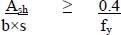
We decide to provide two-legged stirrups of 6 mm diameter as shear reinforcement. The cross-sectional area of this stirrup would be 56 mm2.
Substituting all the relevant values into the expression,
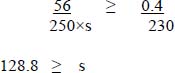
Hence, the spacing for stirrup has been decided as 125mm c/c (center to center).
The section with all reinforcements is shown in Figure 7.13:

Designed RCC section – illustration 7.2
7.4 Design of reinforced concrete slab
Slabs are the plane structural elements, which carry loads primarily by flexure. Slabs form the floors and roofs of building. They are mostly horizontal, though inclined slabs are not an exception and are used for sloping roofs, ramps, etc. Even a staircase in the strict sense is an inclined slab. Slabs may be supported by beams or walls. Further, a slab may be simply supported or continuously supported over one or more supports. Generally, slabs are classified according to the manner of support. Some of the common types of slabs are as follows:
- One-way slabs (spanning in one direction)
- Two-way slabs (spanning in both axes of its plane)
- Flat slabs (supported directly on columns with no beams)
- Ribbed slabs (slabs supported on grid beams)
Out of these, the first two are the most common types of slabs. We will study the design procedure applicable for these two types only.
7.4.1 Design of slabs
Slabs are designed by using the principle of flexure and shear as are used for beams. The following methods of slab analysis and design are available for adoption:
- Elastic method – by idealizing the slabs as strips of beams
- Limit state method – based on semi-empirical coefficients provided in the design codes
- Yield line theory
We will concentrate on the elastic design of slab. While adopting the elastic method for design, the slab is treated as a number of beams placed adjacent to each other, with structural connectivity with each other. Slabs usually are much thinner than beams. The main features of this design approach are as follows:
- Slabs are analyzed and designed as beam components with unit width, i.e., 1 m wide strips.
- Slab sections are usually designed as singly reinforced. Compression reinforcement in a slab is used only in exceptional circumstances.
- Due to large cross-sectional area, the shear stresses are usually very low in the case of a slab. Therefore, shear reinforcement is not provided in slabs. If higher than permissible shear stress is encountered by any chance, the slab section is redesigned by changing the thickness.
- Slabs are always provided with temperature reinforcements (also termed as distribution reinforcements), placed at right angles to the main reinforcements.
A typical slab reinforcement laying is shown in Figure 7.14.

Slab reinforcement
7.4.2 Loads on slabs
The load application on a one-way slab (or for that matter, any slab) can be in the form of uniformly distributed loads or concentrated loads or a combination of both. The slab in residential buildings or other similar structures is predominantly subjected to uniformly distributed loads. Slabs in bridges, in culverts, or in other similar situations are subjected to concentrated load on account of vehicles or trains passing over the slab. Thus, loading on a slab normally consists of the following:
- Live loads
- Dead load of the slab itself
- External dead load (due to finishing, fixtures, fixed equipments, etc.)
Live loads and external dead loads may be obtained from design codes or can be determined by studying the details and nature of loading and collecting relevant data. The dead load, due to self-weight of the slab, is calculated after assigning a probable value for the thickness of the slab
7.4.3 Reinforcement in slabs
As we have observed, in the case of beams previously, certain norms are adopted regarding provision of reinforcements in the slab. They have been described as below.
Diameter and spacing of reinforcement
Some of the norms related to reinforcement bars are as follows:
- The maximum diameter of the reinforcement bar in a slab should not exceed 12.5% of the total thickness of the slab.
- The clear cover for tensile, compressive, shear or any other reinforcement in a slab shall not be less than 15 mm or the diameter of the reinforcing bar, whichever is more.
- Maximum distance between bars should be provided as stated below:
- The spacing of the main tensile bars in the slab should not exceed three times the effective depth of the slab or 450 mm, whichever is smaller.
- The spacing of the distribution reinforcement, provided to guard against temperature and shrinkage in the slab, should not exceed five times the effective depth of the slab or 450 mm, whichever is smaller.
Minimum quantity of reinforcement
The cross-sectional area of reinforcement, in either direction in slabs, should not be less than 0.15 per cent of the total cross-sectional area if ordinary mild steel bars are used as reinforcement. In the case of high strength deformed bars, the minimum value can be brought down to 0.12 per cent of the gross cross-sectional area.
7.4.4 Features of one-way slabs
One-way slabs are those in which the length is more than twice the breadth. When the ratio of the length of a room to its breadth is greater than two, most of the load is carried by the short span (i.e., the width the room) and the slab is designed to span along its width. Due to this, the bending takes place in one direction only, which is along the smaller span. The one-way slab can be simply supported or continuous. The effective spans under different conditions are the same, as those described for beams in the previous section. A continuous one-way slab can be analyzed in a manner similar to that for a continuous beam. For design purposes, a one-way slab is treated as subjected to loads in a manner similar to a beam and, therefore, results in flexural and shear stresses. Shear stresses in slabs are generally not critical under normal loads but should still be checked for safety.
In the case of a one-way slab, the main reinforcements of the slab span the width of the slab, while the distribution reinforcements are laid at right angles to the main reinforcement. The maximum bending moment for which the slab should be designed depends on the span of the slab, loading conditions and the end conditions of the slab. The bending moment which causes tension at the bottom of the slab, usually near the center of the span, is called positive bending moment and the bending moment which causes tension at the top of the slab, usually over the supports, is called negative bending moment. In the case of a positive bending moment, the main reinforcement is placed at the bottom face, while to resist negative bending moment the main reinforcement is placed at the top face of the slab.
7.4.5 Design procedure
The slab design procedure is quite similar to the beam design. The design is undertaken for a width of one meter and the same is adopted for the entire slab. The design procedure for a uniformly loaded, one-way reinforced slab can be divided in the following steps:
The first step in the design is to work out the effective span for the slab, as per the norms pertaining to support size and conditions.
The next step would be to calculate the dead loads and live loads on the slab. Live loads include all temporary loads while dead loads are the permanent loads, which include self-weight, weight of finishings, weight of permanent fixtures, etc. The self-load for the slab shall be assessed by assuming a suitable thickness. It may be remembered here that the load calculation is done per metre width of the slab. With the span as well as the loads known, the maximum bending moment for the slab span would be determined.
Now we start the process of designing the section. In the first step, we would calculate the values of design constants, i.e., k (neutral axis factor), j (lever arm factor) and R (moment of resistance factor) from the given stresses in concrete and steel reinforcement. With the values of maximum bending moment and moment of resistance factor known, the effective depth requirement is calculated from the following equation:
d = √{M/(R × b)}
The value of b is taken as 1000 mm.
If the derived effective depth, and from there the overall depth (D) work out to be different from the depth assumed, the design would need revision from that step onwards. On the other hand, if the effective depth determined this way is compatible with the assumed depth of the section, the same would be adopted for the calculation of steel area.
In the next step, the area of main reinforcement would be calculated from the formula
As = M / (σst×j×d)
With cros-sectional area of each reinforcement bar known, the center-to-center spacing of main bars shall be derived by the formula
s = 1000 × Abar / As
Even if there is a conflict, it would be ensured that the maximum spacing adopted in the design should not exceed 3d or 450 mm, whichever is smaller. The area of distribution reinforcement would also be calculated as per these norms and their spacing decided.
Finally, to check for shear, the percentage area of main reinforcement would be calculated and the permissible shear stress would be determined. This would be compared with the actual magnitude of the maximum shear stress. If the value of the actual magnitude exceeds the permissible value, the design would be revised by adopting a different thickness for that depth of slab.
We will undertake a design exercise to illustrate the procedure.
Illustration 7.3: Design a floor slab simply supported over a clear span of 3.5 m. The length of the slab is 15 m. The slab is to be finished with 25 mm thick concrete flooring. The super-imposed load on the slab would be 4000 N/m2. The bearing of the slab on the supporting walls is 250 mm.

To design the slab section, we need to determine the highest bending moment within the span of the section. Since the ratio of length and width of the slab (15 m and 3.5 m, respectively) is higher than 2, the slab is one way for analysis and design.
We assume an overall thickness of 125 mm at this stage. The effective depth for this section should be very near to 100 mm.
The center-to-center span of the slab, which is 3.75 m, is higher than the sum of clear span and effective depth (3.6 m). Therefore, the effective span for the one-way slab would be 3.6 m.
Considering a strip of 1m width, the self-weight of per meter span of slab would be
ws = 0.125 × 1 × 25000 = 3125 N/m
Similarly, the dead load due to 25 mm thick flooring would be
wf = 0.025 × 1 × 24000 = 600 N/m
The live load per meter span of the slab would be equal to 4000 N/m.

Now, from the data about material characteristics, we will determine the value of k for the section. Using expression,

Moment arm factor,

For the section, the value of coefficient of the resisting moment,

We know that the moment of resistance of the section,
M = Rbd2
The value of M is known and the value of R for the case has been derived. By substituting these values into the expression above,

The effective depth of the slab should be 119.6 mm. We presently have assumed an overall depth of 125 mm, which won’t be able to accommodate this requirement. Therefore, we reject this trial and again try with an overall slab thickness of 150 mm for the slab.
Considering a strip of 1 m width, the self-weight of per meter span of new slab section would be
ws = 0.15 × 1 × 25000 = 3750 N/m
The live load per meter span of the slab would be equal to 4000 N/m.
Total load on slab = Live Load + Dead Load
w = 4000 + 3750 + 600 = 8350 N/m
Maximum bending moment

From relation, M = Rbd2
13527 × 1000 = 0.874 × 1000 × d2
d = 124.4 mm
This requirement of effective depth is compatible with our overall depth assumption of 150 mm.
As we are designing a balanced section, the area of steel required would be derived from the following expression:

Let us provide 10 mm diameter main reinforcement for the slab. The area of each bar would be equal to 78.6 mm2.

This spacing is well below the limit of three times the effective depth of the section, and is, therefore, acceptable. We can provide the 10 mm diameter reinforcement at 80 mm c/c spaced.
Check for cover

This is well above the minimum required norm of 15 mm, and, hence, is acceptable.
Provision of distribution reinforcement
The minimum area for distribution reinforcement for the MS steel is 0.15% of the gross sectional area:
= 0.15% × 1000 × 150 = 225 mm2/m
Since the requirement of steel is small, we would provide 6 mm diameter bars (area 28.27 mm2 for each).

This spacing again is smaller than 3d and, hence, is acceptable. For distribution, 6 mm diameter bars spaced at 125mm c/c would be provided.
Check for shear stress
We know that the maximum shear force would be at either one of the supports.

The percentage of tensile steel in the overall section = 899 / (1000 × 124.4) × 100% = 0.72%.
For the combination of 0.72 percentages of steel, 150 mm section depth and concrete with characteristic strength of 15 N/mm2, the permissible value of shear stress in the section is 0.334 N/mm2 × 1.3.
Hence, the shear force withstanding capacity of the section
= 0.334×1.3×1000×124.4 = 54014 N.
The capacity of this section to resist shear force exceeds the maximum value of shear force at any section of the slab. Hence, the design is acceptable.
The cross section of the slab showing details of the proposed reinforcement is shown in Figure 7.15.
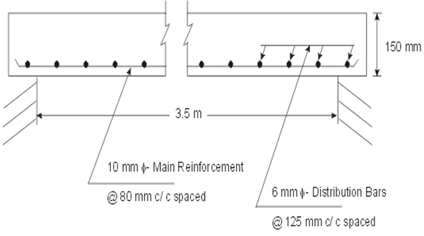
Slab section design – illustration 7.3
7.4.6 Features of two-way slabs
If the length to breadth ratio of the slab is less than two and the slab is supported on all its four sides, two-way spanning action occurs. In this situation, the slab acts as a plate supported all around, with maximum deflection and moment occuring at the centre. Two-way slabs may be simply supported or continuous over any or all supports. The deflections and bending moments in a two-way slab are considerably less compared to those in a one-way slab. Thus, the result is a thinner slab section with lesser amount of reinforcement. If the slab is square, the two-way action remains equal in each direction. As is clear from the description, the slab spans in two directions and, therefore, main reinforcements are provided along both the spans of the slab in a two-way slab.
For the purpose of design, a two-way slab may be considered to consist of a series of interconnected beams. These beams of unit width will transfer the load to the respective supports. The vertical deflection of the central point, which is common to the beams of both the spans, will remain identical. Elastic analysis of two-way slabs is based on this assumption. The exact analysis of stresses in two-way slabs is quite complex. These are generally designed using approximate theories, which are known to yield satisfactory results based on experimental data. For advanced analysis, the finite element method is also used as a tool for the slabs of any shape, boundary condition and subject to any loading. This method can also account for stiffness of the supporting beams and is extremely useful for slabs with openings and those subjected to concentrated loads.
Design procedure
There are a number of procedures to undertake design of two-way slabs. Out of these, the Rankine–Grashoff method is quite effectively and widely used. According to this method, the overall load on the slab is so split up along the X and Y axes that the deflection at the central point, the point common to the strips in X and Y axes, does become the same.
Consider the slab shown in Figure 7.14. The slab has spans lx and ly as indicated in the diagram. The strips at the centre of the slab in both the directions are being considered. The slab is subjected to a uniformly distributed load of w per unit area. This load is simultaneously acting on both the strips and, therefore, it is assumed to be divided into two portions, wx and wy.

We already know that for a simply supported beam, subjected to uniformly distributed load, the deflection at the centre of the span would be 5wl4 / 384 EI. Equating the values of the deformation for both the beams,

Once the distribution of load from these expressions is determined, the further process of bending moment calculation and section design is similar to the one described in the case of one-way slabs.
The one thing worth remembering here is that in the case of two-way slabs, there is no provision for distribution reinforcement as the main reinforcement itself is provided along both the spans. As one layer of main reinforcement shall be provided over the layer in the other direction, the effective depth of the section would be different for the spans in X and Y directions.
Shear force for a two-way slab
As in the case of any beam, the maximum shear force would be at the edge of the slab. For two-way slabs, a uniformly distributed load on the slab is assumed to be transferred on the four edges in the manner indicated in Figure 7.16.

Two-way slab
Design procedure
As shown in Figure 7.16, MNOP is a rectangular slab, with MN and OP being the larger sides (ly) of the slab and NO and MP being the smaller sides (lx) of the slab. The ratio ly/lx has been r.
For the purpose of assessment of load, which would be transferred to each of the edge supports, a line each from M, N, O and P has been drawn at 45º to the respective edge. The lines from M and P meet at Q and the lines from N and O meet at R. These lines divide the entire rectangular area of the slab into two triangles and two trapeziums. The load on each of these areas would assume to be transferred to the edge beam or wall, which is the base of the triangular or trapezoidal shape.
For example, the load on triangular area NOR would be transferred to the edge NO. The area of this triangle,
Area = lx × (lx /2)/2 = lx2/4
If the load per unit area is w, the total load on this triangular portion
= w × lx2/4
Due to this load, the average reaction per unit length at edge
= w × lx2/4 × (1/ lx)
= w × lx/4
However, the maximum reaction near the centre of the edge would be more than the average value. Its value would be equivalent to w × lx/3.
The shear force along the longer edge can also be calculated from the diagram. Once the values of shear force, and hence shear stress, on the slab section are known, the information would be treated for design in the same way as we have seen in the design of a one-way slab.
7.5 Design of reinforced concrete foundations
Foundations are the structural elements that transfer loads from the building or individual columns to the ground on which it rests. This term includes the portion of the structure below ground level (sub-structure), which provides a base for the structure above the ground (super-structure) as well as the extra provisions made to transmit the loads on the structure.
The objectives of providing the foundation are as follows:
- To distribute the weight of the structure over a large area so as to avoid loading of the soil beneath, beyond its safe bearing capacity
- To load the sub-structure evenly and avoid unequal settlement of soil
- To extend the structure deep into the ground and thus increase its stability preventing overturning.
The foundations for buildings may be classified as follows:
- Isolated footings – These are under individual columns and such footings may be square, rectangular or circular in plan.
- Combined footings – These foundations support two or more column loads. These may be rectangular or trapezoidal in plan or they may be isolated bases joined by a beam.
- Raft or mat foundation – These are large continuous foundations supporting a large number of columns of a structure. These are adopted when soil conditions are poor and the risk of differential settlement is high.
- Pile foundations – Piles are narrow sections, which penetrate deep into the soil. These are used in case a good stratum is available at a large depth or the loading conditions are too severe to be taken by the shallow foundations. Pile caps are used to tie a group of piles together. These may support isolated columns or groups of several columns.
The above cover almost all types of foundation systems adopted for buildings. It may be noted that, in addition to the piles, there are some more kinds of deep foundations like pier, caisson and well foundation, which are used for special structures like bridges.
The choice of the type of foundation to be used in a given situation depends on a number of factors, which have been named below:
- Bearing capacity and penetration resistance of soil
- Nature of structure
- Magnitude of loads
- Acceptable settlement norms
In this section, we would focus on the design principles and procedures related to individual spread footings.
As the name suggests, in the case of spread footings, the base of the load-bearing member (a column or a wall) is made wider so as to distribute the load over a larger area, when it reaches the strata at ground. A footing that supports a single column is termed the isolated column footing. It is normally observed that a square footing works out to be economical for square and circular columns. Rectangular footings are considered to be more appropriate for rectangular columns.
The photograph of an isolated column footing being cast with concrete is shown in Figure 7.17.

Isolated column footing
Design criteria for footings
The basic requirements for the design of shallow foundation are as follows.
The area of footing should be so derived that the maximum pressure on the soil does not exceed its safe bearing capacity.
The foundation should be designed in such a manner that the structure does not tilt under loading. If the centre of gravity of the load does not coincide with the center of gravity of footing, the bearing pressure under footing will not remain uniform. There would be higher pressure on the edge of footing nearer to the centre of gravity of the load, which will cause greater settlement of soil at the edge and this can result in tilting of the foundation. This should be avoided by designing the footing area in such a manner that the center of gravity of the load coincides with the center of gravity of footing.
The depth at which the foundation should be located depends on the character of the sub-soil and the magnitude of load on the structure. However, besides taking other criteria into consideration, the foundation must be carried below the following:
- The depth at which high volume changes in soil due to moisture fluctuation does not cause any adverse effect.
- Below the depth of unconsolidated material like muck, garbage dumps and similar other materials
- The depth of frost penetration in a region of temperate climate.
Minimum depth of foundation
The design codes normally specify a minimum required depth for the foundation, keeping in view the stability of the structure. However, if a good stratum is available at lower depth, it is possible to place footing at depth lower than the minimum specified. To decide the depth of foundations for all important constructions, it is necessary to carry out soil investigation of the site. The test report would contain details regarding the type of sub-soil strata at various depths, depth of water table and recommendation regarding the bearing capacity of soil at different depths.
For normal buildings, the depth of foundation below ground level is commonly calculated by Rankine’s formula. According to this, the minimum depth of foundation is given by the following relationship:

Footing design – some norms
The analysis and design of footings involves basically the following steps:
- Determination of the area for footing to transfer weight
- Determination of bending moment and shear force at critical section and freezing the depth of footing
- Determination of the reinforcement steel in the footing section
Some of the general norms followed in the design exercise are as below.
Thickness of footing
In RCC footings, thickness of the block at the edge should not be less than 150 mm for footings resting on the earth. They should not be less than 300 mm in the case of footings constructed over piles (termed pile cap).
Bending moment
1. The bending moment at any section shall be determined by passing through the section a vertical plane across footing and computing the moments of the forces acting over the entire area of footing on one side of such plane.
2. The location of critical sections, where the value of moment bending moment is supposed to be largest, is identified as below.
- For footings supporting a concrete column or pedestal, at the face of such column/pedestal.
- For footings under masonry walls, sections located half-way between the center line and the edge of the wall.
Tensile reinforcement
The total reinforcement at any section should be provided according to the desired moment of resistance of the section, as in the case of any other beam. In one-way reinforced footings, the reinforcement shall be distributed uniformly across the full width of footing. In two-way reinforced square footings, the reinforcement extending in each direction shall be distributed uniformly across the full width of footing. However, for the two-way reinforced rectangular footing, the reinforcement in the long direction shall be distributed uniformly across the full width of footing. For reinforcement in the short direction, a band at the centre of footing and in length equal to the width of footing shall be marked, along the length of footing and that portion of reinforcement determined in accordance with expression given below shall be uniformly distributed across the central band.

Here, β would be the ratio of the long side to the short side of footing.
The balance reinforcement would be uniformly distributed in the remaining portions of footing.
Shear force
When footing acts as a wide beam, the critical section for the shear should be a vertical section, located from the face of the column at a distance equal to the effective depth of footing in the case of footing on earth and a distance equal to half the effective depth of footing in the case of pile caps.
In addition to the normal shear force, footing, which supports a column, is subjected to punching shear. This is a two-way acting shear force, which occurs due to the reason that the concentration of the load transferred onto footing through the column can be quite high and its effect would be to try to penetrate footing.
The punching shear is checked at the distance d/2 from the periphery of the column, where d is the effective depth of footing. The value of shear stress thus obtained should not exceed the following:

where βc is the ratio of short to long side of footing.
If the value of the actual punching shear stress exceeds this value, it would be necessary to redesign the footing section by altering the depth.
We will see the procedure of design of isolated footing and the application of these norms in the below illustration:
Illustration 7.4: The objective is to design a footing for a 300 mm × 300 mm sized column. The load carried by the column is 500000 N. The characteristics of soil and RCC materials are as follows:
| Characteristic Strength of Concrete | = | 20 N/mm2 |
| Permissible Stress in Steel | = | 230 N/mm2 |
| Safe Bearing Capacity of Soil | = | 120000 N/m2 |
| Modular Ratio | = | 14 |
First of all, we need to determine the area of footing necessary for safe transmission of the load from column.

Safe bearing capacity of soil is 120000 N/m2. Hence, the required area of footing:
A = 560000/180000 = 4.66 m2
Since the column section is square, we would provide a square footing for the even distribution of load on the soil.
Length of one side of the square footing = √3.11 = 2.16 m.
Hence, we will provide footing of the plan size 2.2 m × 2.2 m.
The pressure on the soil (and also the upward pressure on footing),
| p | = | 560000 / (2.2 x2.2) |
| = | 115702 N/ m2 | |
| = | 115.7 kN/ m2 |
With upward pressure and the size of footing known, we can calculate the bending moment at the critical section. In this case, the section on the face of the column itself is the critical section. Under upward pressure, the portion beyond the critical section acts as an inverted cantilever with a uniformly distributed load of intensity 115.7 kN/m2 acting on it. The span of this cantilever would be as follows:
L = (2.2 – 0.3)/2 = 0.95 m
The bending moment at the critical section at the column face, for entire length of the section,
| M | = | 2.2 ×w×L×(L/2) |
| = | 2.2 ×115.7 × 0.95 ×(0.95/2) | |
| = | 114.86 kN-m | |
| = | 114860 N-m |
Determination of depth
For the given characteristic strength of concrete, the permissible compressive stress would be 7 N/mm2.
Now, from the data about material characteristics, we will determine the value of k for the section. Using expression,
k = m× σcc
m×σcc+ σst

= 0.298
Moment arm factor,

For the section, the value of coefficient of the resisting moment,
| R | = | j×k×σcc/2 |
| = | 0.9 × 0.298 × 7/2 | |
| = | 0.939 |
We know that the moment of resistance of the section,
| M | = | Rbd2 |
| 114860 × 1000 | = | 0.939 × 2200 × d2 |
| d | = | 235.8 mm |
As we are designing a balanced section, the area of steel required would be derived from the following:
| As | = | M / (σst×j×d) |
| = | 114860× 1000/ (230 × 0.9 × 235.8) | |
| = | 2353 mm2 |
Let us provide a 12 mm diameter main reinforcement for the slab. The area of each bar would be equal to 113 mm2.
| Spacing of the bars | = | 113 × 2200 /2353 |
| = 105.7 mm |
This spacing is well below the limit of three times the effective depth of the section, and, therefore, is acceptable. We can provide the 12 mm diameter reinforcement at 100 mm c/c spaced.
Check for shear
We know that the critical section for shear is the one away from the column face by the value of the effective depth. In this case, the adopted effective depth is 0.227 m.
The magnitude of the shear force at the critical section would be equal to the upward force on the footing area beyond the critical section. The value of shear force would be
| = | 115.7 × 2.2 (0.95 – 0.236) | |
| = | 181.74 kN | |
| = | 181740 N |
The percentage of reinforcement in the footing section,
| = | 2353 /(2200 × 236) × 100% | |
| = | 0.453% |
For 0.45% of steel area, the permissible shear stress in the given grade of concrete would be 0.286 N/ mm2. Also, since the overall depth of the section would be in the range of 275 – 300 mm for this case, shear stress multiplication factor of 1.05 shall be applicable.
Hence, permissible shear stress = 1.05 × 0.286 = 0.3 N/ mm2.
Hence, the shear force resisting capacity of the critical section,
| S | = | 0.3 × 2200 × 236 |
| = | 155760 N |
The value of shear resistance capacity of critical section is less than the total shear force at the section. Therefore, it is needed to revise the design.
Since the shear force-carrying capacity of the section is proportional to the effective area of the section, we can determine the new effective depth with which the section can withstand the total shear. It may be noted that since the likely overall depth of section would increase beyond 300 mm, the shear stress multiplication factor of 1.05 would not be applicable in the case. Also, since the percentage area of steel in the section is going to reduce in the case, we adopt a value of 0.23 N/mm2 as permissible shear stress.
| Effective Depth | = | 181740 / (2200 × 0.23) |
| = | 359.2 mm |
Hence, we adopt an overall depth of 425 mm for footing.
Check for punching shear
The critical section for punching shear is at a distance d/2 from the column edges.
| The value of shear force at the section | = | 115.7 × {2.22 – (0.3 + 0.359)2} |
| = | 509.7 kN |
| Periphery of this section | = | 4 × (0.3 + 0.359) = 2.636 m |
| Value of shear stress at the section | = | 515.8 × 1000 / (2.636 × 359 × 1000) |
| = | 0.545 N/mm2 |
We know that the permissible value of punching shear stress is given by the expression
τps = k × 0.16 ×√Characteristic Strength of Concrete
Since footing is rectangular in plan, the value of k would be 1.
| Hence, | τps | = | 1 × 0.16 ×√20 |
| = | 0.715 N/mm2 |
This value is more than the actual punching shear stress at the section. Hence, the section is safe as per this criterion.
Area of steel
The overall depth of the section has been assumed as 425 mm. Also, the reinforcement consists of 12 mm diameter bars in both the directions. The net effective depth available for the upper bottom layer of reinforcement
| d | = | 425 − 50 − 12 − 12/2 |
| = | 357 mm |
For this depth, the requirement of reinforcement shall be
| As | = | M / (σst×j×d) |
| = | 114860×1000/ (230 × 0.9 × 357) | |
| = | 1555 mm2 |
Again, we provide 12 mm diameter main reinforcement for the slab. The area of each bar would be equal to 113 mm2.
| Spacing of the bars | = | 113 × 2200 /1555 |
| = 159.87mm |
This spacing is also less than the effective depth of the section. Therefore, we can provide 12 mm diameter reinforcement bars @ 150mm c/s spacing.
Check for shear
We will again check the value of permissible shear stress in the section to compare it with the actual value. We know that the critical section for shear is the one away from the column face by the value of the effective depth. In this case, the effective depth is 0.317 m.
| V | = | 115.7 x 2.2 (0.95 – 0.357) |
| = | 150.94 kN | |
| = | 150940 N |
The percentage of reinforcement in the footing section,
| = | 1555 /(2200 x 357) x 100% |
| = | 0.20% |
The permissible shear stress would be 0.22 N/mm2.
| The permissible shear force at the critical section | = | 0.22 × 2200 × 357 |
| = | 172788 |
Hence, the shear capacity of the section is adequate and can be finally adopted.
The section of footing showing details of reinforcements can be referred to in Figure 7.18.

Design of footing – illustration 7.4
7.6 Design of axially loaded columns
As we already know, the columns are the members predominantly subjected to direct compressive force. There can be cases when column sections can be subjected to large flexural stresses (in frames for instance, as shown in the photograph in Figure 7.19), but such cases are not being considered here.
A column is said to be subjected to axial load when the line of the resultant of loads supported by the column coincides with the center of gravity of the column section. Such loading generates only compressive stresses in the column section and in view of concrete’s strength in compression, reinforced concrete is a very useful material that can withstand axial compressive loads. The other positive factor is based on the architectural requirements or the amount of load to be supported. Reinforced concrete columns can be cast in various shapes like square, rectangular, hexagonal, circular, etc. Columns of L-shape or T-shape are also sometimes used in various buildings.

RCC frame: combination of beams columns
As concrete itself is quite strong in compression, the longitudinal steel bars in columns supplement this bearing capacity of the column. In column section, the steel bars are uniformly spaced along the perimeter of the column as near to the surface as permissible. The longitudinal bars are held in position by transverse reinforcement, termed lateral binders. The binders firstly prevent the displacement of the longitudinal bars during concrete pouring operation and further prevent the tendency of their buckling outwards under loads.
Transverse reinforcement in RCC columns can be of two types. The first type consists of individual binders made of small diameter bars, bent around the longitudinal bars and spaced evenly. The diameter, spacing and the profile of such binders depend upon the number and diameter of longitudinal bars and the overall cross-sectional size of the column. In the second type, reinforcing bars are wound around the longitudinal bars in the form of a closely spaced continuous helix and are termed as spiral or helical reinforcements. Apart from rendering support to longitudinal bars against buckling, the helical reinforcement acts to confine the concrete within it. In effect, it forms a core of concrete that increases the load-carrying capacity of the column. Some of the common arrangements of binders and helical reinforcements are shown in Figure 7.20.

Column sections – typical reinforcement
The behavior of RCC section in columns is quite different from its behavior in beams, as we will see later. The following points may be useful to help design an economical and cost-effective column section:
- Columns with separate lateral ties work out more economical than columns with spiral reinforcement.
- While in conformity with all other design norms, the axially loaded column with a low percentage of steel works out more economical for each ton of load supported, compared to the column with a higher percentage of steel as the main reinforcement.
- It is better to avoid lean concrete for compression members. The use of rich concrete mix normally results into economical design.
Types of columns
On the basis of response to loading, reinforced concrete columns can be broadly divided into the following categories:
- Columns with longitudinal steel with individual lateral ties or binders
- Columns with longitudinal steel with helical transverse reinforcement
- Composite columns with a steel structural member encased within the concrete
Of all the above types, columns reinforced with longitudinal steel and provided with lateral ties/spirals are most commonly used. Encased columns are recommended if the load to be carried is very high and the overall dimension of the column section is required to be restricted as a result of space or aesthetic consideration.
Effective length
A column is a compression member and, therefore, is prone to buckling under load. In the case of reinforced concrete, the actual length (L) of a column from practical considerations is taken as the clear distance from the floor and the underside of the beam of the least depth, at the next floor level that frames into the column from any direction. As we have seen in the section on ‘Analysis of Columns’, the effective length (Leff) of the column would be dependent on the end restraints.
The theoretically derived effective length for a column and the values adopted for RCC columns are shown in the table below.
| Nature of End Restraint | Effective Length (Leff) |
|---|---|
| Effectively held in position and restrained against rotation at both ends | 0.5 L |
| Effectively held in position at both ends, restrained against rotation at one end | 0.7 L |
| Effectively held in position at both ends but not restrained against rotation | L |
| Effectively held in position and restrained against rotation at one end and at the other restrained against rotation but not held in position | L |
| Effectively held in position at one end but not restrained against rotation and at the other end restrained against rotation but not held in position | 2 L |
| Effectively held in position and restrained against rotation as one end but not held in position nor restrained against rotation at the other end | 2 L |
Permissible stresses in RCC columns
Based on research, the design codes recommend somewhat lower permissible stresses in concrete and steel in direct compression, compared to the corresponding value in the bending. The reason for it is that unlike in the case of bending, the value of stress remains uniform throughout the section and also remains unchanged from section to section. Consequently, no section gets relief anytime. Hence, there has been no scope to transfer the stress from the higher stress fibres to the adjoining lower stress ones.
The permissible stresses for various grades of concrete and for various type of steel reinforcement, to be considered in the design of column, have been indicated below. The corresponding value of stress in concrete in bending has also been shown for comparison.
Permissible compressive stress in concrete
| Grade of Concrete | In Bending Compression | In Direct Compression |
|---|---|---|
| M15 | 5.0 N/mm2 | 4.0 N/mm2 |
| M 20 | 7.0 N/mm2 | 5.0 N/mm2 |
| M25 | 8.5 N/mm2 | 6.0 N/mm2 |
| M30 | 10.0 N/mm2 | 8.0 N/mm2 |
Permissible compressive stresses in steel reinforcement
For steel bars, the values of permissible stress in direct compression are as follows:
- For ordinary Mild Steel = 130 N/mm2
- For High Yield Strength Steel = 190 N/mm2
Capacity of columns
While determining the load-carrying capacity of the reinforcement concrete column, the capacity of concrete and steel is determined separately and added to determine the combined capacity. This is a deviation from the principle followed for the composite section, where the strain in each of the material remains the same and the load distribution is determined accordingly. The reason for this deviation is the special deformation characteristic of concrete under compression. Concrete undergoes the following three types of strain:
- Elastic strain – The strain due to application of load on the member. This is observed immediately on the application of load.
- Shrinkage strain – Due to chemical reaction, which results into hardening, the concrete undergoes reduction in its volume. This phenomenon is known as shrinkage. Shrinkage is not dependent on load and its effect is observed in the medium term.
- Creep – Creep is a phenomenon special to loaded concrete. As per this, concrete under compression for a substantial period undergoes slow deformation, which is time dependent. The effect of creep can be observed in long term only.
Hence, in the RCC column section, concrete observes strain due to shrinkage and creep, in addition to the usual elastic strain. The effect of these two, on the composite behavior of materials, is quite complex. However, research has proved that it is safe to consider independent load-carrying capacity of both materials in the RCC section.
The load-carrying capacity of various types of columns can be determined as follow.
Short columns
RCC columns are classified as either long or short, based on the ratio of their length and sectional dimensions. A column is considered to be short when the ratio of its effective length to its least lateral dimensions does not exceed 12. If this ratio exceeds 12, the column is considered to be a long column. On account of its tendency to buckle, a long column has less load-carrying capacity than a short column of the same cross-sectional area.
The permissible axial load on a short column reinforced with longitudinal bars and lateral ties is given by the relation
| P | = | σcc× Ac + σsc× As | |
| Here, | σcc | = | permissible stress in concrete in direct compression |
| Ac | = | net cross-sectional area of concrete | |
| σsc | = | permissible compressive stress for reinforcement steel bars | |
| As | = | cross-sectional area of longitudinal steel. | |
The permissible load for columns with helical reinforcement shall be 1.05 times the permissible load for similar members with lateral lies or rings. This provision can be made applicable only if the ratio of volume of helical reinforcement to the volume of core is not less than the value given by the expression
0.36×(Ag/Ac – 1)×(fck / fy).
| Here, | Ag | = | gross area of the section |
| Ac | = | area of the core of the helically reinforced column measured to the outside diameter of the helix |
Long columns
The principle for the determination of load-carrying capacity of a long column is the same as for a short column. However, in long columns, the maximum permissible values of stresses in concrete and steel can be brought down by multiplying the respective stresses by a reduction coefficient, Cr, given by the following formula:
Cr = 1.25 – Leff /48b
| where | Leff | = | effective length of column |
| b | = | least lateral dimension of column |
For more accurate calculation, the following formula for reduction coefficient can also be used:
Cr = 1.25 – lef/160 imin
where imin = least radius of gyration for the column section
Column design – common norms
Some of the commonly accepted norms for RCC column design and detailing are described below:
Longitudinal reinforcement
- The minimum area of cross section of longitudinal bars must be at least 0.8% of the gross cross-sectional area of the column.
- In any column that has a larger cross-sectional area than that required to support the load, the minimum percentage steel must be derived based on the area of concrete required to resist direct stress and not on the actual area provided.
- The maximum area of the cross section of longitudinal bars must not exceed 6% of the gross cross-sectional area of the concrete. However, it is recommended that the maximum area of steel should preferably be kept within 4% to avoid difficulties in placing and compacting of concrete.
- The bar should not be less than 12 mm in diameter, so that it is sufficiently rigid to stand up straight in the column form during fixing and concreting.
- The minimum number of longitudinal bars provided in a column must be four in rectangular columns and six in circular columns.
- Spacing of longitudinal bars measured along the periphery of a column should not exceed 300 mm.
Transverse reinforcement
Transverse reinforcement may be in the form of lateral ties or spirals. They may also be in the form of polygonal links with internal angles not exceeding 135°. All of the transverse reinforcement should be properly anchored. The reinforcement should satisfy the following requirements:
- The minimum diameter of the lateral ties or helical reinforcement shall not be less than ¼ of the diameter of the largest-sized longitudinal bars with a lower limit of 5 mm.
- The maximum diameter of the ties should preferably be not more than 12 mm as it requires bending to the desired shape and size.
- The pitch of the ties, which is the longitudinal distance between two adjoining ties, should not exceed the smallest of the following.
- The least lateral dimension of the column
- 16 times the smallest diameter of the longitudinal reinforcement bar to be tied
- 48 times the diameter of lateral tie or transverse reinforcement
- The pitch of the helical turns should not be more than 1/6 of the core diameter up to the centre of helix or 75 mm, whichever is lower.
The illustration below would demonstrate the process of RCC column design in accordance with all the stated norms.
Illustration 7.5: A 7.5 m long column is hinged at one of its ends and fixed on the other end. The total vertical load acting on the column is 600000 N. It is required to design the reinforced section for this column.
The design data are as follow:
| Characteristic strength of concrete | = | 20 N/mm2 |
| Permissible direct compressive strength in concrete | = | 5 N/mm2 |
| Permissible direct compressive stress in steel | = | 190 N/mm2 |
For these end conditions, the effective length of a column would be 0.7 times the actual length.
Hence, Leff = 0.7 × 7.5 = 5.25 m.
We make a trial with the section of 300 mm × 300 mm for this column.
Gross area of the section = 300 × 300 = 90000 mm2
For this section, the ratio Leff/b is as follows:
Leff / b = 5.25 ×1000 / 300 = 17.5.
Since the value of Leff/b is more than 12, the column would be classified as a long one.
The stress reduction factor for the section,
| Cr | = | 1.25 – Leff /48b |
| = | 1.25 – 5.25 ×1000/ (48 × 300) | |
| = 0.885 |
Reduced Permissible Stress in concrete = 0.885 × 5 = 4.425 N/mm2.
Reduced Permissible Stress in steel = 0.885 × 190 = 168.15 N/mm2.
We need to determine the area of steel required for the section. If this is assumed as As, the load capacity of the column would be
P = 4.425×(300×300 – As) + 168.15× As
Equating this to the actual load on the column,
| 600000 | = | 4.425×(300×300 – As) + 168.15× As |
| As | = | 1233 mm2 |
We provide 20 mm diameter bars (area 314 mm2 for each) for the section.
Number of bars = 1233 / 314 = 3.92.
Hence, we provide four 20 mm diameter bars, which meet the criteria for the minimum number of bars for a column section.
The next step is to design the transverse reinforcement. The diameter of the tie bar should be larger than ¼ of the main bar’s diameter or 5 mm. For 20 mm diameter, the value derived from both the criteria is 5 mm. Hence, we provide ties of 5 mm diameter.
To decide the distance between the ties, we know that the pitch should be the least of the following three:
- The least lateral dimension of the column : 300 mm in this case
- 16 times the smallest diameter of the longitudinal reinforcement bar: 16×20 = 320 mm for this case
- 48 times the diameter of a lateral tie or transverse reinforcement: 48×5 = 240 mm for this case.
Since the least value of the three is 240 mm, we provide 5 mm diameter lateral ties @ 240 mm center to center along the longitudinal axis of the beam.
The sectional details of the column are shown in Figure 7.21.

Column reinforcement details – illustration 7.5
7.7 Pre-stressed concrete – an introduction
Although the composite behavior of steel and concrete in reinforced concrete structures is an excellent combination for the two materials, still there are certain deficiencies inherent in the combination. The most significant of these is that the concrete in the tensile zone of the section does not theoretically contributed towards the strength of the member and is required to be completely ignored. Its sole function is to bind the reinforcement in place and transfer the tensile load to these. The same weakness of concrete in tension prevents the use of very high tensile steel for reinforcement, as in the process of transferring the tensile force to the reinforcement, the RCC member can develop wider than permissible cracks in the concrete on the tension side of the beam. This crack formation, in turn, can lead to the corrosion of reinforcement due to contact with atmospheric moisture and, hence, may affect the stability of the member.
7.7.1 Pre-stressing of concrete
To overcome the above limitations of RCC work, the process of pre-stressing of concrete is adopted. In principle, pre-stressing means the introduction of stress in the material, opposite in nature to the stress induced by loading, prior to loading of the member. As a result of this, the stress induced by loading is neutralized by the pre-stress available in the member, partially or fully.
In the case of concrete, in view of its weakness in tension, sufficient compressive stress is introduced during pre-stressing prior to the member being subjected to loads. Consequent to this, when the pre-stressed concrete member is subjected to external loads, the already induced compressive stress in concrete would neutralize the tensile stresses developed in the tensile zone of the section. The resultant stresses in the concrete in the tensile zone would either be eliminated altogether or get reduced to a very large extent. Thus, the entire cross section of the member becomes effective for resisting bending and at the same time the danger of cracking, when the load is minimized or avoided.

Principle of pre-stressing
The stress development in sections of a pre-stressed concrete member is illustrated in Figure 7.22. The normal section under loading and subjected to bending would have tensile and compressive stresses as shown. Now in addition, if a uniform compressive stress in introduced in the section such that its magnitude is exactly equal to the tensile stress post loading, the combined effect would be the elimination of tensile stress from the section. Of course, the magnitude of maximum compressive stress would definitely become higher in this case, but this is an acceptable situation, in view of the high available compressive strength of the concrete.
In this situation since no tensile stress is present, the section does not need any steel as reinforcement. In this regard, the pre-stressed section is different from the RCC section and has similarity in behavior with a homogeneous material like steel.
7.7.2 Advantages of pre-stressed concrete over reinforced concrete
The advantages of a pre-stressed concrete member over a conventional reinforced concrete member can be summarized as below:
- By pre-stressing, it is possible to take full advantage of the high compressive strength of concrete for resisting loads. At the same time, the high tensile strength steel is used to introduce pre-stress in the concrete. The combination of these two materials in this fashion leads to a more economical section compared to an RCC section.
- The pre-stressed member can better withstand the effect of impact and vibrations.
- In view of elimination of tensile cracks in the pre-stressed concrete members, they have increased resistance to atmospheric action and the structural durability increases.
- Pre-stressing leads to leaner members, in section, compared to RCC for similar loading conditions, which reduces the weight of the structure and ultimately effects economy in the cost of foundations.
- The pre-stressing induced in the concrete member tends to reduce diagonal tension. The use of curved tendons contributes to the shear strength of a pre-stressed member.
At the same time, it may be noted that the procedure of pre-stressing is quite sophisticated and requires proper equipments and highly skilled workmanship. Due to this, the concept is not feasible for small structures. Pre-stressing has succeeded as an alternative to RCC for heavily loaded, long-span sophisticated structures like bridges and industrial sheds. It requires an elaborate setup to undertake pre-stressing work; as we will see in further sections, the process is not quite feasible for smaller structures. It can almost be said that pre-stressed concrete is an alternative to reinforced concrete for some structures, which are specialized in nature and are large enough to be termed as of optimum size.
7.7.3 Materials
The materials used in a pre-stressed concrete member are:
- Concrete
- Steel
Concrete in pre-stressed concrete
The concrete used for a pre-stressed concrete member is normally of higher strength than the same used for RCC members. Generally, concrete with characteristic strength equal to or in excess of 30 N/mm2 is used for pre-stressed construction. The reason for it is that it is possible to utilize the full strength of concrete in such structures and the incremental cost to produce high strength concrete over a relatively a low strength concrete is favorably low. It is also possible in the case of high strength concrete to allow a small amount of tensile stress in the extreme fibre of the section. In addition, high strength concrete has a high value of modulus of elasticity (Ec), which results in smaller deformation in the members. Research has also proven that a rich mix of concrete has a lower value of creep deformation, which reduces the ultimate loss in the pre-stressing force.
Steel in pre-stressed concrete
The steel used in pre-stressed concrete has the function to induce compressive force in the concrete section. To achieve this, the steel is stretched through a mechanism and then locked in place. This steel under tension induces the compressive force of required magnitude in the concrete section. Pre-stressing steel is generally used in the form of individual wire, termed tendons, with a high tensile strength. It is not feasible to use low or medium strength steel as tendons since the losses in the pre-stress are quite large and that itself may exceed the permissible stress limits of these steels.
The diameter of the commonly available hard drawn steel wires ranges from 1.5 mm to 8 mm. These tendons have an ultimate tensile strength ranging from 1400 N/mm2 to 2350 N/mm2, depending on their diameter.
7.7.4 Losses in pre-stressing
It has been observed that the pre-stressing force, induced in a concrete member, does not remain constant throughout. It actually decreases with the passage of time on account of various causes. The important causes of loss in pre-stressing force are the following:
- Loss due to elastic shortening of concrete – Concrete, like any elastic material, undergoes a deformation when stressed. This is recoverable and the amount of which depends on the stress induced as well as the modulus of elasticity of the material. The shortening of concrete due to this reason releases a part of the tensile force in the tendons.
- Loss due to shrinkage of concrete – As we know, concrete undergoes shrinkage due to the chemical reaction during hydration of cement. This again releases some stress from tendons in the medium term.
- Loss due to creep in concrete – The creep in concrete results in the shortening of a concrete member under constant compression. The effect on stress in tendons is similar to that in the case of shrinkage.
- Loss due to creep in steel – Creep is also observed in steel under constant loading. The effect of it is the plastic strain in steel that results into loss of stress up to 5% of the original stress.
- Frictional loss – This is the loss due to the friction present between the tendons and the material surrounding it to transfer the load to the concrete. This is applicable only to post-tensioned members.
- Loss due to slip at anchorages – A slight slippage takes place when the load is shifted from the stretching mechanism to the anchorage. This also results into loss of stress in steel up to a certain degree.
The cumulative effect of all such losses may be as high as 15% to 20% of the initial pre-stressing force. Therefore, allowance is required to be made at the design stage itself to account for all these losses while determining the tensioning force to which tendons have to be stretched. Therefore, it is obvious that the effective pre-stressing force, acting on a section, will be equal to the pre-stressing force initially applied to the concrete less the sum of the overall losses of pre-stress, which can be caused by the above-stated factors.
The following illustration would make the concept of pre-stressed concrete design further clear:
Illustration 7.6 : A concrete beam is subjected to bending moment of 80kN-m. The beam is being designed as a pre-tensioned pre-stressed concrete member. Concrete has a characteristic strength of 45 N/mm2 and the 1.5 mm diameter tendons of high yield strength are used. The objective is to design a suitable section.
The design constants are as follows:
| Permissible flexural compressive stress in concrete | = | 15 N/ mm2 |
| Permissible flexural tensile stress in concrete | =1.5 N/ mm2 | |
| Losses in pre-stress | = | 15% |
Let us consider a concrete section of 300mm width and 500mm depth for the purpose of the first trial.
We know that the section modulus (Z) for a rectangular section,
| Z | = | bd2/6 | = | 300×(500)2/6 |
| = | 12500000 mm3 |
And the flexural relationship,
Bending Moment M = Z×f.
Hence, 80×1000×1000 = 12500000 ×f.
From this, f = 6.4 N/mm2.
This means that the concrte section is subjected to 6.4 N/mm2 stress in its extreme fibres on both tension and compression sides. Since concrete cannot withstand tensile stress in excess of 1.5 N/mm2, it can withstand the compressive stress up to 15 N/mm2. Therefore, the pre-stress in concrete has to be adusted accordingly.
Let the value of pre-stressing force on the entire cross section be C.
Then, 6.4 + C/(300×500) = 15
which gives the value of force as 1290000 N or 1290 kN.
And 6.4 – C/(300×500) = 1.5.
This limiting case provides the value of C as 750000 N or 750 kN.
Since the second case meets the limiting condition pertaining to tensile stress in concrete at a smaller load, the value of 750 kN can be adopted for design purpose. Also, since the losses in pre-stress are 15%, the value of pre-stressing force required in the case,
F = 750 / (100 –15)%
F = 883 kN
Therefore, tendons with area to withstand 883 kN force would be provided.
The section tried above may be adopted with the magnitude arrived for the pre-stressing force. It may, however, be noted that the section has potential to withstand higher moment, which can be exploited by providing higher cross-sectional area of the tendons.
7.7.5 Methods of pre-stressing
The pre-stressing of concrete can either be done at the stage of casting itself or at a time when the concrete has hardened sufficiently. Based on this, the method of pre-stressing can be classified as follows:
- Pre-tensioned method
- Post-tensioned method
Method of pre-tensioning
In this method of pre-stressing, the tendons are placed on the casting bed in the already designed pattern, tensioned up to the design limit and finally fixed with the anchor posts, provided at each end of the casting bed. The framework is erected around it and concrete of a required grade is placed in this framework. Once the concrete gets hardened and develops the desired strength, the connection between tendons and the anchor posts is released. On account of the bond between steel and concrete, the tendons transfer the induced force to the concrete, thereby compressing the hardened concrete in the member. In some cases, depending upon the quality of steel and the diameter of the wires used, the bond between steel and concrete alone may not be sufficient to prevent the tendons from returning to their original position after the concrete has set. In such cases, special anchorage treatment is provided at the ends of the member.
This method is commonly adopted for pre-stressing simply supported slabs, beams, fence posts, etc.
Method of post-tensioning
Unlike pre-tensioning, in the post-tensioned method, the pre-stressing force is applied to the tendons after the concrete has hardened and has acquired the necessary strength. As is obvious that the tendons cannot have a direct bond with the hardened concrete before tensioning, a grouting material is filled around the tendons post tensioning. The tendons are pulled through ducts or grooves left for them in the precast concrete member. The pulling or stretching of the cables or tendons is done with the help of jacks acting against the ends of the precast member.
The method of post-tensioning is applicable for heavy pre-stressed concrete members like bridge girders. The photograph of an under construction post-tensioned pre-stressed concrete bridge is shown in Figure 7.23.

Pre-stressed concrete bridge – under construction
There are various systems to apply post-tension in a precast concrete member. Some of the more popular systems are the Freyssinet System, the Lee–McCall System, the Gifford–Udall System and the Magnel–Blaton System.

Post tensioning system – tendons at the end
The procedure of pre-stressing is the same in all the systems except that the details of the tendons and method of providing anchorages differ. In all the important systems, the cables and the hydraulic jacks used for stretching the tendons are especially designed for a particular pre-stressing work. The photograph of one such system with tendons at the end is shown in Figure 7.24.
7.8 Multistoried structures
The RCC is widely used for the construction of multi-storied buildings, all over the world. The construction of one such building is shown in Figure 7.25. The design and analysis of such multistoried structures is rather cumbersome as a large number of joints need to be analyzed with lots of forces acting on them. In addition, the number of frames has a large number of joints, which are free to move, so the amount of effort involved in the analysis becomes tremendous. Usually, the analysis of multistoried structures is carried out by taking one floor at a time. It is assumed that the shear and bending moments on one floor have negligible effects on the floors that are above and below it. Most of the times, a small portion of the frame – called substituting frame member – is taken into account to calculate all the moments and reactions acting on it.
As the numbers of stories are constructed over one another, the dead load of the floors above has to be carried by the structural members underneath. The live loads on the top floors also get transferred to the bottom floors.

RCC multistoried structure – under construction
In addition to all the usual dead, live and shear forces, the wind forces and horizontal forces due to seismic effect are taken into account while designing a multistoried structure. These forces cause vertical forces in columns and moments in all the members. During the analysis it is assumed that all of these horizontal forces are transferred to the joints. The common methods used for analysis are:
- Portal method
- Cantilever method
- Factor method
Shear and axial forces in all of the members of the structures are calculated by any one of the above-mentioned methods. Thereafter, the design of each member is completed as per the standard requirements.

Composite building construction
It must also be emphasized here that besides pure RCC, a number of times steel too is used in combination to design and construct high-rise building and structures. This process of using more than one prime material in construction is known as the composite construction method. The basic concept describing the same is shown in Figure 7.26.
Design and analysis of multistoried structures, RCC as well as composite, is a topic of advanced design procedures and is out of scope of this chapter.
7.9 Conclusion
We are now in a position to easily appreciate the versatility of concrete, its ingredients, manufacturing and its various characteristics, which have usefulness in design and construction of reinforced concrete structures.
In this chapter, we gained familiarity with the design principles for reinforced concrete, which theoretically is a composite construction. We can appreciate the behavior of reinforced concrete under different kinds of loadings and predict the response of the material.
Specific to the structure, we have understood design principles and procedures for beams, slabs and compression members. These are the basic elements of an RCC structural system and understanding of their design can make one appreciate the entire design process, which would be undertaken in the design of large and complex structures.
At the final stage of the chapter, we have been introduced to pre-stressed concrete. This provides knowledge about another dimension in which the properties of concrete are being exploited for better and more economical construction.
This chapter will help the reader to appreciate and use the limit state method, a design philosophy that has been rapidly getting the preference over working stress philosophy, due to the economy and degree of optimization it brings in the design outcome.
Learning objectives
After completion of this chapter, one will be able to:
- Understand the basic philosophy and uniqueness of the limit state design
- Understand its application in the design process
- Use the principle to design certain structures in RCC as well as in steel
In the previous chapters, we have studied the design process by applying basically the working stress and ultimate design theories. We also got introduced to the limit state design principles. In the current chapter, we would understand the philosophy and its application in further details.
8.1 Limit state theory
As we observed, the various design principles, in their application ensure that the parameter identified as critical is not exceeded during the lifetime of the structure. This parameter happens to be the induced stress in the working stress method and the load applied in the ultimate load method.
Under the limit state philosophy, the design objective is to achieve a reliability of acceptable degree that the structure will not reach the state of failure and non-serviceability, called limit state.
As stated, the limit state can pertain to the safety as well as serviceability requirements. In other words, one category defines the conditions when the structure is assumed to have reached the stage of failure or collapse. The other category defines the conditions when the structure though is away from the failure, its use for the purpose intended can be a problem.
8.1.1 Limit state of collapse
The limit state of collapse corresponds to the situation when a clearly defined structural usefulness limit has exceeded, though it may not necessarily result into an actual collapse. Such limit of collapse may correspond to the following:
- Flexure
- Compression
- Shear
- Torsion
8.1.2 Limit state of serviceability
The limit state of serviceability corresponds to the situation when the structure has reached a level of physical deformation that it turns non-acceptable for intended use, though the structural failure might not have occurred yet. The limits of such collapse may correspond to the following:
- Cracks
- Deflection
- Vibration
8.2 Design philosophy
Under the working stress or plastic failure theories we studies earlier, the emphasis had clearly been on one structural theory. However, the limit state method is not identified with any particular structural theory. Based on the limit state under consideration, the most applicable theory is adopted during the analysis. In addition, the probabilistic variation in the loading, as well as in the structural properties of materials, is also captured during the analysis phase.
As per limit state principle of design, the limit state of collapse is expressed by the following expression:
k × R ≥ λ × L
Here,
| k | = | Factor of Safety |
| R | = | Resistance or Capacity of the structure |
| λ | = | Load Factor |
| L | = | Load |
To explain, if the structure is subjected to a single type of load that has the maximum potential value of L during the lifetime of the structure, the same needs to be designed for a situation equal to λ times the load. Further, the resistance offered by the structure would be k times of such modified load. Therefore, the tolerance is being provided both ways: first while assessing the loads to take care of uncertainty associated with them and second while determining the resistance.
It must be noted that in the case of multiple loading on the structure, the expression above will take the following form:
It is worth recollecting that in the case of working stress method, the factor of safety is applied only on the resistance side. In other words, unlike working stress method, the limit state design method recognizes that there exists a degree of unpredictability about the loads the structure is likely to encounter during its lifetime and it needs to be taken care of. It is established that the structure designed in accordance with the working stress method will have varying safety margins as against the limit state method in which loading system is assessed for various limit states and separate safety factors are employed for different loads.
The other notable difference between the working stress and limit state method is in the way they deal with the stress as a function. In the working stress method, as we know, the stress generated in the member is compared with the maximum permissible stress to make judgment. In the limit state method, the stress in the member due to duly factored set of loads is obtained to determine the design strength and assess the safety of the member.
Further, in order to take care of limit state of serviceability, the following general expression is used:
| Here, | Δ | = | Deflection of the member |
| L | = | Length/span of the structural member | |
| a | = | A constant |
This, in theory, is similar to the philosophy adopted in the working stress method of design.
8.3 RCC design by limit state
The limit state method of design takes into consideration the probabilistic variation in the loads as well as in the physical properties of material. Without going deep into statistical aspects, it would be useful to understand some commonly adopted terms associated with the process.
8.3.1 Characteristic values
The characteristic values, as described below, are associated with the nature of material and load conditions.
Characteristic Strength: The term pertains to the material of construction: in this case, it is concrete. The difference in the strength of various samples may not be large, but it is imperative to express these by way of statistics. For this purpose, the characteristic strength implies a minimum value which at least 95% of the specimen are expected to exhibit. In other words, not more than 5% of the specimens are expected to fail below this value.
The same is true for the reinforcement steel, too.
In order to elaborate further on this, one may refer to Figure 8.1, in which a typical Gaussian distribution of concrete specimen strength is shown. Mathematically, it can be shown that the criteria of less than 5% failure is satisfied if
σk = x − 1.64 σ
| Here, | σk | = | Characteristic strength |
| x | = Arithmetic mean of the results | ||
| σ | = Standard deviation |

Distribution curve – characteristic strength
In the case of concrete, the characteristic strength is represented by the 28-day compressive strength of cube specimens. For steel, depending on its composition, it either remains the yield stress or 0.2 % proof stress.
Characteristic Load: For the purpose of design, the characteristic load is taken as the one which has 95% probability of not being exceeded during the lifetime of the structure.
Again, from statistics, the value of characteristic load can be described as

| Here, | wk | = | Characteristic load |
| x | = Arithmetic mean of the loads | ||
| σ | = Standard deviation |
8.3.2 Design values
While adopting the values of characteristic strength as well as the characteristic loads for design, relevant factors are applied on them. The design value of each is derived as follows:
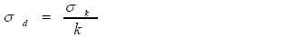
In this expression, k is a partial safety factor appropriate to the material.
Similarly, the value of design load is expressed as follows:
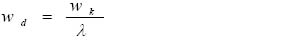
Here, λ is the partial safety factor appropriate to the loading.
The use of adjective partial may be noticeable, with the term ‘safety factors’. The reason to qualify them as such is that in the case of limit state design, different safety factors are applied for different materials as well as for different loads.
For material’s strength, the adoption of safety factor is dependent on factors like degree of probability of strength variation, possibility of section size variation, consequences of failures, etc. As is obvious, steel being a factory-produced item fares better than concrete on these fronts and, therefore, a lower safety factor of 1.15 is adopted for steel against 1.50 for concrete.
In the case of loads, the safety factors are required to take care of instances like accidental increase in loads, inaccurate assessment of loads and stress redistribution. Since the probability of such occurrences is different for different load types, the safety factor allocation for each also varies.
The generally adopted values of partial safety factors for different load conditions are provided in Tables 8.1 and 8.2.
| Load Combination | Partial Safety Factors Recommended |
|---|---|
| Dead Load plus Live Load | Dead Load – 1.5 Live Load – 1.5 |
| Dead Load plus Wind Load | Dead Load – 1.5 Wind Load – 1.5 |
| Dead Load plus Live Load plus Wind Load | Dead Load – 1.2 Live Load – 1.2 Wind Load – 1.2 |
| Load Combination | Partial Safety Factors Recommended |
|---|---|
| Dead Load plus Live Load | Dead Load – 1.0 Live Load – 1.0 |
| Dead Load plus Wind Load | Dead Load – 1.0 Wind Load – 1.0 |
| Dead Load plus Live Load plus Wind Load | Dead Load – 1.0 Live Load – 0.8 Wind Load – 0.8 |
The above list is not exhaustive. For instance, for serviceability limit state of overturning, where dead load acts as a restoring force, the partial safety factor for dead load adopted is lower than one.
8.3.3 Material properties
Before describing the design process, it may be useful to look at behavior of the RCC ingredients under stress. Concrete is the main ingredient and its behavior under stress depends on factors like mix proportion, age, physical properties of aggregates, shape and size of member, etc.
The actual stress–strain curve for a concrete specimen is considered as too complex to be useful for design purpose. To overcome this, an idealized stress–strain curve is used, as shown in Figure 8.2. As shown, the top one, with parabolic shape near ultimate value, is the idealized curve based on behavior of test specimen. The same has been reproduced in the middle by applying a reduction factor of 0.67 to take care of variation between specimen and actual site concrete. The partial safety factor, as shown in the bottommost curve, has been applied over and above this factor.
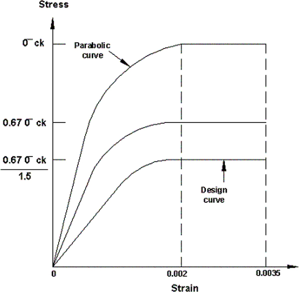
Idealized stress–strain curve for concrete
The other important design characteristic for concrete is the modulus of elasticity (E). In the case of concrete, this value is dependent on the similar value for aggregate, the aggregate-cement proportion, extent of loading, etc. For the design purpose, the modulus of elasticity in compression is expressed as a function of characteristic strength. ACI-318 expresses the value as per the following expression (however, a variation of 80% to 120% of the same is expected in the actual practice):
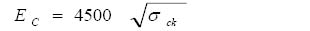
Here, σck = 28-day compressive strength of concrete in N/mm2.
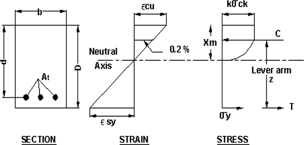
Idealized stress–strain behavior in limit state
In the case of steel, the other important ingredient of RCC, the stress–strain relationship and idealized form have already been described in an earlier section on RCC design. It can be mentioned that a lower partial safety factor (1.15 usually) is applied over yield stress to determine the design value.
An idealized version of stress–strain behavior adopted for RCC section in limit state is shown in Figure 8.3.
8.3.4 Collapse stage
Any RCC structural member is designed in such a way to withstand the stresses induced by the load application. In the case of beam section subjected to lateral load, we already know that reinforcement concrete acts as a composite material and withstand the flexure effectively. When the RCC beam is subjected to gradually increasing load (and not impact), the section passes through different phases before reaching a failure state. These stages are as follows.
- Uncracked state: In this state, the maximum stress in concrete, tensile as well as compressive remains less than the required for rupture. In such case, the value of stress can be derived by the expression
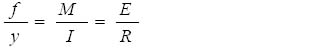
Here, f is the value of maximum stress induced due to moment M. The other notations mean the typical values.
At this stage, the limit state as well as working stress approaches yields the same results.

Relationship – moment/curvature
- Cracked state: Once the load reaches a stage that the bending moment induced by it is in excess of the cracking moment of the section, the concrete in the tensile phase develops crack and loses its ability to withstand the tensile stress. In such case, the tensile force starts getting transferred to the reinforcement bars. However, the bond between concrete and steel remains intact to enable the section act as a single composite one.
- Collapse stage: As the stress value keeps on increasing in the cracked state, a stage reaches when the stress in the reinforcement steel reaches its yield or limiting value. This is termed as stage of collapse. Here, unlike in the working stress method, the concrete in compression is expected to fail only when the strain in it exceeds the limiting value that has been derived empirically to 0.35%. The analysis of this state is important from the design perspective. The approach of relating concrete failure to limiting strain rather than limiting stress value optimizes the process better.
The relationship between moment and the deformation (by way of curvature) for all the three stages is shown in Figure 8.4.
Also, to physically relate it with the strain values, the relationship between moment and strain in all stages is shown in Figure 8.5.

Strain–moment relationship in RCC
8.3.5 Analysis – limit state
To analyse the reinforced concrete section subjected to flexure under limit state of collapse, the following assumptions are made:
- The plain section before bending remains plain after bending, too
- The stress–strain relationship in concrete is assumed to be parabolic, with maximum compressive stress being equal to 0.67 times the characteristic strength
- The maximum value of strain in concrete is taken as 0.0035, irrespective of the grade of the concrete
- The tensile strength of concrete is assumed as nil
- The stress in reinforcement steel is taken either as the function of its yield strength or as the proof strength, whatever may be the case
- The maximum permissible strain in tensile reinforcement steel should not be less than the value given in the below expression:
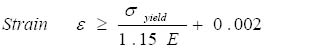
The distribution of strain across the typical singly reinforced RCC section is shown in Figure 8.5.

RCC – stress distribution
Let us take the case: when this beam is subjected to a load, the factored value of which is capable of generating ultimate or collapse bending moment in the section. The stress–strain relationship is shown in Figure 8.6. The reinforcement is subjected to the yield stress (factored with 1.15). The stress in concrete follows a parabolic distribution to a depth x1 and then remains constant up to its ultimate value. The value of strain corresponding to parabolic stress limit and ultimate limit is 0.2% and 0.35% respectively.
With partial safety factor of 1.5, the ultimate stress in concrete = 0.67 ςck.
Also, if the total depth of compression zone is x, then
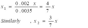
Total compressive force = due to parabolic bloc + due to rectangular block.
Assigning values,
Compressive force C = 0.542 σck b x
Applying partial safety factor of 1.5 for concrete,
Safe compressive force Cs = 0.36 σck b x
The following can be derived further from the diagram and analysis:
Depth of neutral axis,
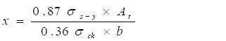
Here At = Area of steel in tension.
Lever arm for a balanced section,

Moment of resistance of section,
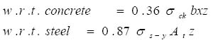
These values, as stated, are applicable for a balanced reinforced section. The values would vary in the case of under reinforced and over reinforced sections.
The method of analysis is illustrated below.
Illustration 8.1: An RCC section of overall size 250 mm x 400 mm is shown in Figure 8.7. We need to determine the moment of resistance of the section.
The relevant strength values are as follows:
For steel: σ s-y = 415 N/mm2
For concrete: σ ck = 20 N/mm2
In order to find the moment of resistance, we first need to assess the depth of neutral axis.
Here,
Area of steel – At = 3 x 201 = 603 mm2
Maximum tensile force,
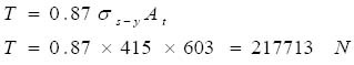
Depth of neutral axis,
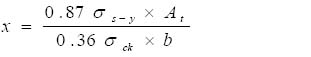

RCC section
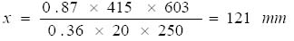
| Lever arm z | = 360 – 0.42 x 121 |
| = 309 mm |
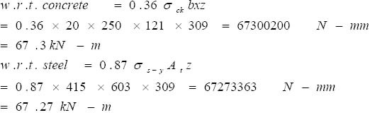
The values derived from both concrete and steel are quite near to each other and hence the section is near balanced. For the purpose of design, the lower of the values, i.e., 67.27 kN-m, can be adopted.
8.3.6 Serviceability limit state
It is already mentioned that apart from satisfying the collapse conditions of limit state, the structure is also expected to satisfy the serviceability conditions of limit state.
The following are important parameters of serviceability.
- Control of deflection: The excessive deflection in the structure does affect its appearance or utility in an adverse way. To describe these conditions, almost all building codes adopt the ‘span ratio’ measure. The maximum permissible deflection of the member is expresses in terms of span/length of the member. It takes into account the deformation due to temperature, creep, shrinkage, etc. As the deflection is a function of sectional area as well as its length, codes do specify the span/depth ratios to be followed during the design.
For instance, as per British Standards, the set of recommendations made is given below:

- Control of cracking: The excessive cracking not only affects the appearance but also can lead to corrosion. Generally, surface width of crack should not exceed 0.3 mm. In an aggressive environment, the surface width should be limited to 0.4% of the clear reinforcement cover.
It must be noted that the analytical method to determine potential cracks is quite cumbersome. Therefore, for general conditions, the design codes normally specify the minimum reinforcement spacing in the tensile and flexure zone, which is suppose to limit the cracks.
- Control of slenderness: A slender member, which has its breadth much lower than the depth, may have a tendency to buckle under load. To check this, the design codes put certain restrictions by way of limiting relationships between length/span of the member and its lateral dimensions.
Besides these, parameters like vibration, etc., can also be covered under serviceability limit state in specific instances.
8.4 Steel structural design – plastic theory
The limit state theory is applicable to steel structures, too. As per limit state theory, the structures are likely to be subjected to various types of loads and deformations arising from service requirements that may range from the routine to the extreme/accidental. The objective of the structural designer is to design a structure that can withstand such demands throughout its expected lifetime.
As we know, the structure is required to have an adequate margin of safety against such demands, the safety factor being necessary to account for various uncertainties due to natural variability, inaccuracy in procedures used for the evaluation and control of loads similar uncertainties in structural resistance (capacity) and its determination.
The structural design criteria for steel, under limit state theory, are based on plastic collapse or ultimate strength. The simplified design of many types of structures relies on estimates of the plastic strength of components, usually from their elastic buckling strength adjusted by a simple plasticity correction.
The safety margin of structures can be evaluated by a comparison of ultimate strength with the extreme applied loads. To obtain a safe and economic structure, the ultimate load-carrying capacity as well as the design load needs to be assessed accurately. The plastic analysis and design procedure have been elaborated in the below subsections.
8.4.1 Plastic theory for design of steel structures
We already have been introduced to the theory of plastic design in one of the earlier chapters. This theory is based on the behavior of steel under load, beyond the stage of elastic deformation. The stress–strain relationship for mild steel, from a typical tensile test, is shown in Figure 8.8.
As per the diagram, from the zero load point 0 to the limit of proportionality point P, the stress–strain relationship is linear. From point P to the yield point Yp, the stress–strain relationship deviates from the straight line and assumes a curved shape. Beyond the yield point Yp, the stress–strain curve still remains non-linear, but becomes much flatter. During this stage, the resistance of steel increases due to strain hardening till it reaches the ultimate strength point U. The stress beyond yield point is not recorded realistically, since the area of cross section of the test piece decreases. Therefore, the strength of steel seems to decrease beyond the ultimate stress point U up to the point of failure.
The basis of elastic theory of design is that under design load the actual stresses in the structural members are always less than the allowable stresses. The theory of elasticity can be used for rational analysis of structures under any system of load within the elastic zone. However, at ultimate load, the stresses within the member would exceed the elastic limit. Therefore, the theory of elasticity will not be applicable for structural analysis at the time of failure.

Stress–strain relationship for mild steel
The main drawback of the elastic design theory is that it does not provide a uniform overload capacity for all parts of the structures. The plastic design or the ultimate load design is nowadays preferred over the elastic theory, since it offers more simplicity and economy in the design of structures.

Idealized stress–strain relationship for mild steel
In plastic design, the strength of material beyond its elastic limit is also used. An idealized stress–strain curve is used to undertake design of structures. This curve, formed of only straight lines, is shown in Figure 8.9. It may be noted here that it is on the conservative side to assume the material to be perfectly elastic, up to a stage, and perfectly plastic beyond that, in turn ignoring the strain-hardening phenomenon completely.
Plastic design of beam
We now observe a case: when bending moment in increasing magnitude is applied on a beam section. As shown in Figure 6.34, the change in stress distribution across the section would be as follows.
Stage – I: Elastic Stage
During this stage, the maximum extreme fibre stress due to bending moment remains within the elastic range. Also, the neutral axis will pass through the centroid of the section.
Stage – II: Elastic–Plastic Stage
When the bending moment is increased further, the magnitude of stress across the section keeps on increasing. At one stage, the stress at the extreme fibre would exceed the yield stress. During this stage, the neutral axis would no longer pass through the centroid of the section (except for sections that are symmetrical about both the axes). The bending tensile and compressive forces on the section would however remain equal.
Stage – III: Plastic Stage
As the moment is further increased, the curvature M/EI also increases and the yielding of fibres spreads, from the extreme edge to inside the section. With a further increase in bending moment, a stage would arrive when the yield spreads along the entire cross section and the section is fully plasticised. The corresponding bending moment is called the plastic moment of resistance and is denoted as Mp. The neutral axis of fully plastic section passes through the equal area axis.

Plastic stage – stress distribution along the section
The development of stresses during these stages is graphically represented in Figure 8.10.
Determination of plastic moment
The plastic moment, Mp, of a section is defined as the maximum moment of resistance of a fully yielded cross section. To make its evaluation simple, the following assumptions are made:
- The material obeys Hooke’s law till yield value. The value of stress remains constant during further elongation.
- The yield stresses and the modulus of elasticity have the same values in compression as in tension.
- In both elastic and plastic states, the material remains homogeneous and isotopic.
- The plane transverse sections remain plane and normal to the longitudinal axis after bending.
- The cross section of the beam is symmetrical about an axis through its centroid parallel to plane of bending.
- Shear strains are neglected for the analysis.
- For a particular section, tension is equal to compression and the net force on the section is always equal to zero.
- Every layer of the material is free to expand and contract longitudinally and laterally under the stress independent of the other layers.
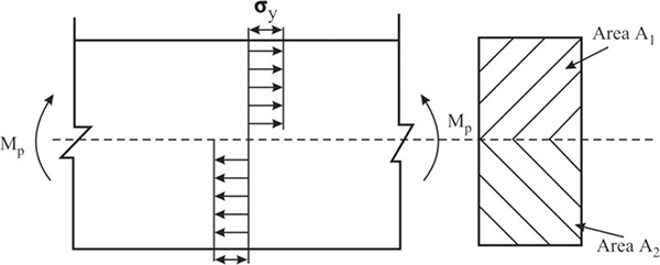
Beam section – yield condition
Consider a beam section, subjected to fully plastic moment M as shown in Figure 8.11. Let A1 and A2 be the areas of cross section above and below the neutral axis while c1 and c2 are the distances of their respective center of gravity from the neutral axis. The yield stress under tension as well as compression is ςy.
| In this case, | ||
| Compressive force on the cross section | = | A1 ×σy |
| And tensile force on the cross section | = | A2 ×σy |
To establish equilibrium in the section,
Compressive force = Tensile force
A1 ×σy = A2 ×σy
Hence, A1 = A2 , which is in line with our assumption.
Also, since A1 + A2 = Total Sectional Area ‘A’,
A1 = A2 = A/2
The Plastic Moment at the section,
| Mp | = | A1 ×ςy×c1 + A2×ςy×c2 |
| = | A/2 ×(c1 + c2) ×ςy | |
| = | Zp × ςy |
The expression Zp is known as the Plastic Section Modulus.
We know that the normal moment-carrying capacity of similar section would be
M = Z × ςy
The ratio of plastic moment capacity to elastic moment capacity would be
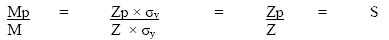
The ‘S’ is termed as shape factor and has different values for different sectional shapes. The shape factor related the plastic moment-carrying capacity with the elastic moment-carrying capacity of the section.
Plastic hinge
When the plastic moment is developed at any section of a structure, the section is completely yielded. Due to characteristics during yielding, the fibres carrying bending, compressive and tensile stress in magnitude equal to yield stress tend to deform continuously. The curvature at the section becomes infinitely large. At this moment, the section continues to rotate at constant moment and starts acting like a hinge. This virtual hinge is known as plastic hinge. Plastic moment allows infinite rotation under a constant moment, equal in magnitude to the plastic moment of the section. Hence, plastic hinge can be defined as a yielded zone, due to bending in a structural member, at which the infinite rotation can take place at a constant moment. Opposed to a mechanical hinge, the moment-carrying capacity for which is zero, the plastic hinge allows free rotation at constant plastic moment. Theoretically, though, the length of a plastic hinge is zero, the values of moment at the adjacent section of the yield zone are more than the yield moment up to a certain length of the structural member. This length is known as the hinge length.
Load factor
In plastic design, ultimate or collapse load is the basis of design of a structural member. The collapse or ultimate load is arrived at, by multiplying the working load We by the load factor. Thus the load factor accounts for the margin of safety in plastic design. The collapse or ultimate load is
Wu = Load Factor × We
In plastic design, the load factor normally provided is 1.65. In elastic design, when the structure is subjected to occasional loads (e.g. wind or seismic loads), the maximum allowable stresses are increased by a certain percentage. A similar effect in plastic design is achieved by adopting a reduced load factor.
Failure condition for plastic analysis
In the case of a plastic structure, the failure occurs due to its conversion into a mechanism. When an elastic body is subjected to load and internal resistance is developed against deformation, the body is termed as structure. In case no resistance is set up in the body against the deformation, then the system is known as the mechanism.
When a structure is subjected to load and the load is gradually increased, those sections with a peak moment will reach the yield point first. The value of bending moment reaches Mp at these sections and plastic hinge formation takes place. As further load is added, the value of bending moment at these sections remains unchanged while values of moments at other sections increase. With increasing load, the value of bending moments at other sections reaches Mp in succession. This phenomenon is known as the redistribution of moment. If the degree of indeterminacy of the structure is r, then the indeterminate structure becomes a determinate structure on the formation of r number of the plastic hinges. If one additional hinge is formed, after the structure has become a determinate one, then a mechanism is formed. Thus, a (r + 1) number of plastic hinges are necessary to convert a structure into a mechanism. The structure fails as soon as it is converted into a mechanism. The load corresponding to the formation of the first plastic hinge is known as yield load, Wy. The load corresponding to the formation of a mechanism is known as collapse load, We.
In the case of plastic analysis, reaching the following conditions would be considered as a failure situation.
- Mechanism formation – The number of plastic hinges developed should be just sufficient to form a mechanism.
- Moment condition: The bending moment at any section of the structure should not exceed the magnitude of plastic moment of the section.
- Equilibrium condition: As per the equilibrium condition, the algebraic sum of all vertical and horizontal forces acting over a structure should be zero. Similarly, the moment of all the forces acting over a structure about any point should be zero.
Types of mechanisms for plastic analysis
The various types of failure mechanisms are as follows.
- Beam mechanism: In this, the location of plastic hinges would be the sections subjected to loads or the sections where shear force changes its sign. The number of plastic hinges would exceed the degree of indeterminacy by one. For instance, in the case of a simply supported beam, the formation of a single hinge would convert the structure into a mechanism. For propped cantilever, it would need two hinges to convert the system into a mechanism.

Plastic analysis – failure mechanism
- Sway mechanism: This mechanism is applicable to frames and the formation of plastic hinges takes place at the joints and at the fixed ends.
- Gable or mixed mechanism: In certain cases of frames, the potential locations for plastic hinges can exceed the value of indeterminacy by more than one. In such cases, there can be more than one potential failure mechanism, one of which is a combination of beam and sway mechanism. This combined mechanism is known as the gable mechanism.
These mechanisms are shown in Figure 8.12.
Procedure for plastic analysis of structures
The plastic analysis for a structural system is the process of determining the value of the largest possible magnitude of the load, which a structure can withstand without collapse. The collapse can be caused either by the failure of a part of the structure or by an overall structural collapse. The part failure can be due to the value of moment at any section exceeding the plastic moment. The overall collapse is the result of the formation of a sufficient number of plastic hinges, which converts the structure into a mechanism. Both the aspects need separate evaluation for structural arrangements. The following theorems are used for this purpose:
Static or lower bound theorem
The static theorem or lower bound theorem is one of the basic theorems of plastic analysis. As per this theorem, for a given frame and loading if there is any distribution of bending moments throughout the frame, which is both safe and statically admissible with a set of loads, W, the value of W must be less than or equal to the collapse load, We.
In the theorem, the statically admissible distribution of bending moments satisfies all the conditions of equilibrium. The safe distribution of bending moment satisfies the condition that the bending moment at any section is not more than the plastic moment of the section.
The process for determination of lower bound collapse load is as follows:
- Convert the structure into a statically determinate one by removing redundant forces.
- Draw the bending moment diagram for this determinate structure.
- Further draw the bending moment diagram for the determinate structure, which is loaded by the redundant forces.
- Draw the combined bending moment diagram, in such a way that a mechanism is formed.
- Calculate the value of ultimate collapse load by solving equilibrium equations (equations of statics).
- Check that the bending moment at every point in the structure is less than or equal to the plastic moment capacity Mp.
Kinematic or upper bound theorem
The kinematic or upper bound theorem states that for a given structural frame subjected to a set of load, W, the value of W, which is found to correspond to any assumed mechanism, must be either greater than or equal to the collapse load.
In practice, if the actual collapse mechanism is known for the given frame and loading, the value of collapse load can be determined by equating the work done by the external loads, during a small motion of the collapse mechanism, to the work absorbed by the plastic hinges. The principle of virtual work is used for this purpose. It states that if a deformable elastic body is in equilibrium under a system of external loads and remains in equilibrium while it is subjected to a small virtual deformation, the external virtual work done by the external forces acting on the body is equal to the internal virtual work of deformation done by the internal stresses.
In the case of actual collapse mechanisms, it would be seen that the values of collapse load obtained separately by the static theorem and by the kinematic theorem are equal. However, if the actual collapse mechanism is not known, possible collapse mechanisms are assumed in such situations. The actual value of collapse load would be the least out of these determined values.
The process for determination of upper bound collapse load is as follows:
- The first step is to set the possible locations of plastic hinges, such as load points, frame joints, maximum bending moment points, etc.
- Select the independent and combined mechanisms. The number of independent mechanisms would be equal to H – r
where H = number of potential plastic hinges,
and r = degree of indeterminacy. - Generate and solve the equilibrium equations for virtual work. Find the maximum collapse or ultimate load for forming a mechanism. The lowest load forming a mechanism is the upper bound of collapse load.
- Check that the bending moment at every point in the structure is less than or equal to the plastic moment capacity, Mp.
To understand it clearly, let’s see the application of the above principles, in the case of a simply supported beam.
As shown in Figure 8.13, a simply supported beam of span L is subjected to a unit load of magnitude W at the centre of its span. The plastic moment capacity of the beam is Mp.

Plastic failure in beam
We know that the maximum bending moment would occur at the centre of the beam span. Hence, the formation of a plastic hinge at the centre is a limiting case. As per static methods, the value of this moment has to be equated to Mp.
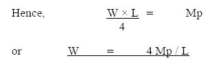
We will determine the value of collapse load as per the kinetic theorem, too. In this situation, the beam mechanism is formed due to the formation of a plastic hinge at the centre. If the slope of the deflected beam at both the ends is θ, the deflection of the beam at the center would be equal to L/2 × θ. The work done by the external load to move this distance

And the work absorbed by the plastic hinge, which has been formed at the centre,
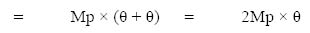
As per the principle of virtual work, the work done by the external load would be equal to the energy absorbed by the plastic hinge.
Hence, W × (L/2 × θ) = 2Mp × θ
or W = 4 Mp / L
The values determined by both the upper bound theorem and the lower bound theorem are the same and are therefore the actual values of the collapse load. The similarity of the values indicates that the failure mechanism assumed in the situation is the actual mechanism.
To illustrate the procedure fully, let us take up another example given below:
Illustration 8.2: The frame in Figure 8.14 is subjected to a load system as shown. The plastic moment capacity of the entire frame is Mp. The objective is to determine the collapse load.

Portal frame under loading
The number of potential locations for plastic hinges is five in this case: one each at the four nodes and another one at the centre of the beam. Against it, the degree of indeterminacy for the frame is only three. Hence, there can be two possible mechanisms for failure.
- Beam mechanism – The beam mechanism is shown in Figure 8.15. The slopes at both the ends are equal. We will straightaway apply the principle of virtual work and equate the work done by the work absorbed.
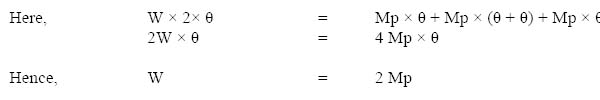

Plastic failure mechanisms – frame
II. Sway mechanism – This mechanism is also shown in Figure 8.15. According to this, the formation of plastic hinges is at both the fixed ends and the beam–column joints. Again as per the principle of virtual work,
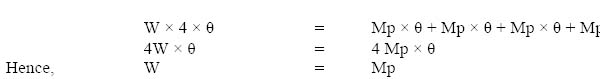
III. Gable mechanism – Apart from these two conditions, the frame may also collapse due to formation of mixed mechanism. This possibility is shown in Figure 8.15. According to this, one of the joints would not reach the plastic moment stage and maintain its rigidity. Instead, the hinge formation would be at the centre of the beam. Applying the principle of virtual work to this condition,
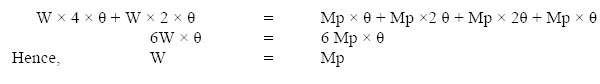
The least value of collapse load obtained from the above analysis is equal to Mp. Hence, it is the actual collapse load value.
8.5 Conclusion
In this chapter, by way of limit state we have gone through a structural design theory that has been gaining wider acceptance due to the overall optimization it brings in the design process. In addition, the emphasis here is given to the actual use situations and not merely to the theoretical aspect of analysis. The structural engineers, all over the world, have been adopting the limit state principles in their design.
This chapter will help the reader to understand the behavior of masonry and timber as structural materials and acquire familiarity with the design and construction principles for both of them.
Learning objectives
After completion of this chapter, one will be able to:
- Understand the use of masonry as a structural material
- Understand the general principles of design of masonry structures
- Understand the characteristics and classification of timber and its use as a construction material
- Familiarize with the design and construction techniques of timber structures
Masonry and timber have been used in construction for a very long time. Though their importance as construction materials in the present day is certainly low when compared to steel and concrete, the frequency of their use is still significant. Therefore, it is useful to understand the design and construction practices related to them.
9.1 Masonry structures
The word masonry implies any structure built by a mason, in which the skill of joining blocks of material with bonding agents is used, such that the ultimate structure acts as a monolith under specified loading conditions.
9.1.1 Materials for masonry
Masonry consists of working with the following materials.
Bricks –

Brick masonry under construction
- These are molded earthen blocks baked to obtain strength and hardness. The earth for the brick is selected carefully and has sufficient content of silica and alumina. Baking is done in large kilns or clamps, using coal or wood as combustible materials. The process of baking takes several days to complete and the final product has enough strength and shape stability, rendering it fit for use as a structural material. A typical brickwork is shown in Figure 9.1.
- The bonding in brick masonry is created with either cement mortar or lime mortar. In cement mortar, cement and graded sand are mixed in a specified proportion (1:3 to 1:6) and water is added to generate a paste like consistency. Lime mortar is prepared in the same way, but lime (calcium hydroxide) is used instead of cement. As lime has practically no tensile strength in comparison to cement, the joint with lime mortar cannot withstand even some amount of tensile or shear force and is therefore used only for small and less important structures. Grooves are maintained in the bricks to create a strong joint.
Stone –
- Natural stones have a very high degree of strength and durability and can be used for masonry structures. The stones can either be of irregular shapes (random stone masonry) or can all be cut into regular shapes and sizes (ashlar stone masonry). The mortars used for stone masonry are the same as those used in brick masonry. Being a natural material, no grooves can be maintained in stones.
- A random rubble masonry work is shown in Figure 9.2.

Random rubble masonry
Concrete blocks –
- Plain pre-cast concrete blocks, solid or hollow, are also used for the purpose of masonry. The blocks are cast and cured in advance so that they achieve a certain desired level of strength before handling. Cement mortar is used for bonding these blocks. Grooves may or may not be maintained in the concrete blocks.
- A typical block masonry work is shown in Figure 9.3
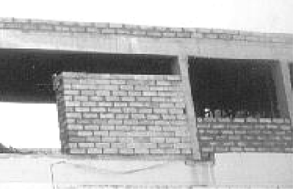
Block masonry
Apart from these common materials, blocks made of certain other materials, such as fly ash, siporex, etc., are sometimes used.
9.1.2 Types of masonry structures
In masonry, the following types of structures are commonly constructed:
- Load-bearing walls
- Arches
- Retaining walls
- Dams
Vertical load-bearing walls are the most common masonry structures. Either brick or stones can be used for the construction of load-bearing walls. As is evident from the name, the predominant loads acting on this structure are vertical loads. In almost all cases, the walls support the roof over them, which can either be a pitched roof or an RCC slab. The wall remains under compressive force due to these loads. The design criterion is the maximum permissible compressible stress in the masonry wall.
Arches are curved masonry constructions in elevation, which support vertical loads of masonry or slabs over them. Arches are provided over an opening and obviate the need of a beam. Due to the nature of their construction, arches are not subjected to bending. Instead, the material is subjected to direct compressive stress as the vertical load acting on it tries to straighten the curved shape. Due to this, arches transfer a large amount of horizontal thrust on the support that needs to be considered carefully in the design. As arches give a better architectural view, those are preferred in place of beams at various locations.
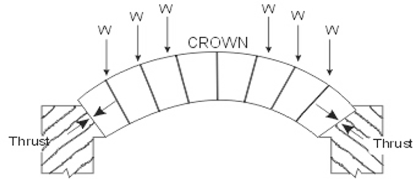
A typical arch
Figure 9.4 illustrates a typical loading on masonry arch and its behavior under loading. The photograph in Figure 9.5 shows the construction of a stone masonry arch.

Stone arch construction
Retaining walls are structures that support earth fillings and are used for maintaining surfaces at different elevations on either side of it. The material supported by the retaining wall is known as the backfill. The backfill of a retaining wall may have its top surface horizontal or inclined. The position of a backfill lying above a horizontal plane at the top level of a retaining wall is termed surcharge.
Dams are constructed structures that retain water on its one side. A dam can either be straight in plan or can have a curved shape. The curved dam acts as an arch in a horizontal plane and is duly termed the arch dam. The masonry dams are mainly subjected to water pressure, which acts horizontally.
Apart from these, chimneys and slabs are some of the examples of masonry structures.
9.2 Design of masonry structures
As we already know, masonry structures can safely withstand compressive loads as the application of such loads does not adversely affect the stability of the structure. Hence, masonry structures are generally designed so that there is only compressive force acting between the blocks of which the masonry is composed. Although mortar in the masonry has some tensile strength, it is common practice to assume the tensile strength of mortar as zero. Therefore, the shear or tangential force on the masonry at any level must not be greater than the natural friction between masonry constituents. The stability of masonry structures is primarily derived from their weight. According to this principle, the dimensions of the masonry structures are so determined that the structures remain stable when subjected to lateral forces.
In modern days, ultra-thin masonry walls are sometimes constructed, which are supposed to carry only their own dead load. The design of these walls is simpler than the usual load-bearing masonry walls. In the case of brick masonry, the effectiveness depends on the pattern in which bricks have been laid, termed as ‘bonds’. Some of the popular brick masonry bonds are shown in Figure 9.6.

Common masonry bonds
The following general conditions should be satisfied in the case of all masonry structures to ensure their stability.
- There must be no tension across the cross section of the structure. If tensile force is generated, it would either separate the two layers of masonry or separate the structure from its foundation.
- The maximum compressive stress must be within the safe limit for the material.
- The shear force must not be greater than the natural friction between the masonry constituents.
- The restoring moment acting on the structure (due to self-weight and dead loads) must be greater than the overturning moment (due to external loads, normally acting laterally).
We will see how these conditions can be met at the design stage.
The first condition is about the generation of nil tensile stress within the section. Refer to Figure 9.7, which shows the cross section of a masonry structure. Point C is the centroid of the cross section. Let the lateral pressure acting on the structure be H; let gravity force be W; and line of pressure cuts the cross section at the load point M at a distance a from C. The resultant force acting on the cross section is R. Let the area of cross section of the masonry structure be A.
In this situation, the direct compressive stress at the section under consideration,
fc = W/A
The cross-sectional area is also subjected to bending moment M due to eccentricity of the gravity force W,
M = W×a

Cross section of a masonry structure
The generation of tensile stress due to the bending moment M,
ftb = (M/I)×xt
If the radius of gyration of the section is equal to k, the value of the moment of inertia
I = A×k2
Then, ftb = (W×a/A×k2)×xt
The net tensile stress due to the combined effect of moment and vertical load on the section is
ft-net = (W×a/A×k2) ×xt – W/A
ft-net = W/A (a×xt / k2 – 1)
The above is the expression of tensile stress at the extreme of the section. Since W/A cannot be zero, the value of (a×xt / k2–- 1) should be equal to zero to fulfill this condition by equating it to zero:

or a = k2/ xt
This general condition has to be met for the cross section of the masonry member to prevent the development of tensile stress within the section.
We will see the specific conditions for common geometric sections that arrive from the above expression.
In the case of a rectangular section of breadth b and depth d:
| k2 = I/A = (bd3/12) / (bd) = d2/12 | |
| And, | xt = d/2 |
Substituting these values into the expression a = k2/ xt:
a = (d2/12) / (d/2)
a = d/6
Hence, to meet a no-tensile-stress requirement for a rectangular masonry section, the point of application of the resultant force must lie within the middle one-third depth of the section.
To derive the value of maximum compressive force, we would pick up the previous analysis from the stage of stress development due to the application of moment.
The compressive stress development due to moment,
fcb = (W×a/A×k2) ×xc
The net compressive stress due to the combined effect of moment and vertical load on the section is
fc-net = (W×a/A×k2) ×xc+ W/A
fc-net = W/A (a×xc/ k2 + 1)
The value of this combined compressive stress should always be ensured within the specified limit.
The further stated requirements of internal frictional force being greater than the shear force and the restoring moment being greater than the overturning moment are easier to analyze and impose. In the first situation, the vertical load multiplied with the coefficient of friction (µ) for masonry on masonry should exceed the value of the lateral force.
Hence, W×µ > H
In order to meet the second of the above-stated requirements, the moment produced by each of the forces acting on the structure, about a point, is calculated. The sum of all the restoring moments, which try to keep the structural stable, should always exceed the sum of all the overturning moments, which tend to make the structure unstable.
| Hence, | Restoring moment Overturning moment |
= | Factor of safety. |
The value of this factor of safety can be 1.2 to 1.5, depending on the type of structure.
9.3 Timber construction
Wood, when used as a structural material, is termed timber. As stated earlier, timber is one of the earliest construction materials. At present though, timber is one of the several materials used in the construction of various types of structures. It is an organic material and is normally used in its natural state, though processed variants are also increasingly used nowadays.
A typical timber construction, with all major structural elements in wood, is shown in Figure 9.8. Besides, some relatively constructions like bridge piers, too, are constructed in timber. One such pier is shown in Figure 9.9.

Timber beam–column roof construction
In view of its low cost, timber is a favored for temporary structures like concrete-form work, scaffolding, sheds for different purposes, etc.

Timber bridge pier
The limited resistant to weathering also encourages its use in temporary works. At the same time, properly seasoned and good-quality timber is successfully used for permanent structures, too. Timber is used for the construction of various structures and structural components such as beams, floors, trusses, purlins, columns, poles, etc. The main advantage of timber over other structural members is its low dead (self-) weight. A typical timber structural erection is shown in Figure 9.10.

Erection of timber structure
9.3.1 Life cycle of wood
It is important to understand the life cycle of wood to appreciate the factors that influence its characteristics. As a natural phenomenon, a fresh layer of new wood is formed every year on the periphery of the tree trunk. The layer is called the annual ring. The increase in the width of the tree trunk is due to the growth of this new wood. The trunk of a young tree consists entirely of light-colored wood, known as sapwood. The sapwood carries sap or juice from roots of the tree to the leaves. This wood contains living cells. With the increase of the age of the tree and the addition of new layers every year, the older wood ceases to take part in the growth activity and its cells die. At this stage, the wood is known as heartwood. This has a distinct dark color and is more resistant to decay. Consequently, it is more durable than sapwood. On the other hand, for the same moisture content, sapwood is stronger and heavier than the heartwood. Sapwood can be impregnated with preservatives more readily because of its absorptiveness.
With regard to the various properties of sapwood and heartwood, the general order of preference for their use is as follows.
- Untreated heartwood of high durability.
- Treated heartwood of moderate and low durability.
- Heartwood of moderate durability after pressure impregnation.
- Sapwood of all classes of durability after thorough treatment with preservatives.
9.3.2 Quality of timber
Teak, rosewood, etc., are common types of woods used for structural purposes. In addition to these, there are a large number of other types available that possess characteristics allowing them to be used as a structural material. Being a natural material, timber usually carries certain defects. To understand it clearly, any irregularity that is present in a specimen of timber can adversely affect its strength, durability or appearance, known as a defect. Timber is seldom entirely free from defects.
The defects in timber may be classified into two types.
- Natural defects
- Defects due to external reasons
Natural defects
Defects that arise due to irregularity in the tissues of the wood are classified as natural defects of timber. Some typical natural defects in wood are described below.
Knots: If either a branch or a limb, part or full, embedded in the body of a tree is cut, then a knot is formed in that wood piece. Almost always, knots are composed of inferior wood than normal wood and the grains are irregular and distorted around the knot. The knots reduce the strength of timber, the extent of which depends upon the size, position and type of knots. In timber beams, the strength is reduced considerably when the knots are situated in the tension zone of the beam. The adverse effect is less if the knots are situated in the compression zone of the beam.
Wane: A wane is the lack of wood or insufficient wood at the edge or corner of a piece of timber. Wane affects the strength of a timber member since the cross-sectional area is reduced. It can be avoided by properly squaring the edge.
There are several other natural defects that affect the strength of the wood.
Defects due to external reasons
Certain defects in timber develop during its lifetime because of the activity of external agents during treatment of sawn timber. Flaws like faulty seasoning techniques may lead to permanent distortion in the timber. This permanent distortion results in various types of warping in timber, as well as the rupture of tissues.
Some of these defects have been described below.
Warping – Warping is caused as a result of permanent distortion of timber. It can be in the form of twisting, cupping or bowing. Warping, which takes place along a spiral shape in the longitudinal direction, is known as twisting. Its taking place along the width of a timber board is known as cupping. When it takes place in the form of sagging from one end to the other along the longitudinal direction, it is known as bowing. Warping reduces the strength of timber, as applied loads do not remain parallel with or perpendicular to the grain.
Rupture of Tissues – The rupture of tissues takes place as a result of permanent distortion of timber. The rupture of tissues includes checks, shakes and splits. A check is a crack or lengthwise separation of the timber. During drying of wood, the outer fibres shrink more than the inner fibres due to which cracks develop across the annual rings. A shake is a separation along the grains of the timber. A split is separation of the timber that extends from one face to the other.
9.3.3 Grading of timber
In order to grade timber for its quality, the defects within timber, their size, amount, and locations are taken into consideration. The density of timber and the effect of slope of grains of timber are also considered.
Timber is graded into the following three categories.
- Select timber
- Standard timber
- Common timber
Select timber is one which is either entirely free from defects or has minimum defects. Standard timber has defects within specified limits. Common timber is inferior to standard timber. Considering the values of the safe working stresses for standard timber as 1, the corresponding values for select timber would generally be 1.15 times. Similarly, the safe working stresses for timber of common grade in compression, shear and bending arc is 0.84 times the safe working stresses for timbers of standard grade.
Any of the grades of timber with defects such as loose grains, splits, heartwood rot, warp, worm holes, pinch pockets, etc., are prohibited from being used as structural members. However, wanes are permitted in structural wood, provided they are not combined with knots. Also, the wormholes (other than those due to powder post beetles) located and grouped to reduce the strength of timber should be treated for evaluation in the same way as knots.
9.3.4 Decay in timber and preservation techniques
The disintegration of timber due to the action of destroying agents is known as decay. Fungi, borers and insects are the common timber-destroying agents. Fungi are the most destructive of the lot. They are a kind of plant that grows in damp places. It travels through the timber and ultimately renders the timber to powder. If the timber is subjected to the cycle of alternate wetness and dryness or is used in dark, damp and unventilated conditions, the fungi get an opportunity to grow. That is the reason why timber has more longevity if maintained either completely dry or completely wet during its lifetime.
Timber structures, which are used for marine works, are subjected to attack by marine borers. They bore into the timber and destroy its strength.
Apart from these, timber deteriorates by the attack of white ants or termites.
In view of the above threats to timber that can lead to decay, it becomes necessary to preserve the timber by using proper methods. The pores of timber are filled up by preservatives, which remove the moisture by penetrating below the surface. Various antiseptic chemical compounds are injected into timber to fill up pores. Coal tar creosote is the most common preservative used. It is also known as creosote oil or dead oil of coal tar. The process of preserving timber by this method is known as creosoting. Plain coal tar is more suitable for surface application. It is applied hot on the outside surface of the timber, especially on the surface that is going to remain in contact with masonry. Mercuric chloride is also used as a preservative. It is injected into the pores of timber and protects the timber from ants and sea worms.
In addition to the above, sodium fluoride, zinc chloride and copper sulphate are some commonly used preservatives.
9.3.5 Seasoning of timber
Seasoning is the process of expelling or drying up the sap present in green timber. This process improves the strength of timber and also increases its durability and stiffness. Seasoning of timber is done either by exposing it to natural air or by placing it in water or hot air. In natural seasoning, bulks of timber are stacked in layers under cover and free circulation of air is allowed around each bark. In water seasoning, timber is placed in water for up to fifteen days. Afterwards, it is allowed to dry thoroughly in the shade. The sap of timber is carried away by water. Another method of seasoning of timber is by placing timber in chambers and circulating hot air around it. The hot air method is effective in reducing the time necessary for seasoning but it is considerably expensive as compared to other two methods.
9.4 Strength of timber
There are a number of factors affecting the inherent strength of the timber. One of the most important is the grain property of timber.
Grain is the term used to denote the direction of fibres of timber in relation to the main axis of a tree or structural member. It also denotes the relative width of annual rings. When the direction of fibres of a tree is more or less parallel to its axis or the longitudinal axis of the member, the grains are called straight grains or parallel grains. These are shown in Figure 9.11. The strength of timber along the straight grains is always higher than along other directions.

Straight or parallel grains of timber
If the direction of fibres within the wood is at varying and irregular direction in relation to the main axis, the grain is termed irregular grain. Irregular grains mostly occur locally and reduce the strength of timber. When the grains are straight but inclined to the main axis, they are termed diagonal grains. The case of diagonal grains is mostly due to improper sawing. If the fibres take a winding or spiral course, such grains are termed spiral grains. These are a serious structural defect and they make the timber weak. Wavy grains are situations where the fibres take the form of waves and undulations.
Apart from the grain condition, the strength of timber is influenced by moisture content, density and the presence of defects within the wood. Moisture is a very important factor influencing the strength. The cell spaces in the green timber would have moisture within. In addition, there would be the absorbed moisture in the cell walls. When green wood dries, free moisture evaporates first. The stage when all the free moisture has evaporated is known as the fibre saturation point. At the fibre saturation point stage, the weight of moisture in the wood remains in the range between 20% and 28% of the dry weight of wood. When the moisture content in the wood is more than the fibre saturation point, the strength of wood practically remains constant. The strength starts increasing when the moisture content of the wood goes below this point. This is accompanied with the loss in volume or shrinkage in the wood. The strength of wood continues to increase until the wood is bone dry.
The density or weight per unit volume of wood indicates the amount of wood substance in a given volume. The strength of wood depends on the amount of wood substance. Dense wood has more strength than lightwood.
The strength of timber reduces due to the presence of defects, which we have already seen in the previous section. The strength of timber also depends upon the size of timber. Defects developed during seasoning in large pieces are more than those in smaller pieces.
9.4.1 Allowable stresses in timber
The allowable or working stresses for timber depend upon a number of factors. The working stresses for any structural material are based upon the basic strength and appropriate factor of safety. The basic strength is obtained by tests on small clear specimens of standard grades in the laboratory.
Being a very diverse material, the design codes normally link the values of allowable stresses for timber with a number of factors.
These factors are:
- Intrinsic quality of the timber
- Location of the structure – Exposure to weather
- Direction of force application – Along or across the grains
- Slope of grains – For grain slopes in between parallel and perpendicular to the axis
- Duration of loading – Wood has lower capacity to take prolonged loads
The factor of safety for timber structures is adopted according to the strength of timber, effect of moisture, the presence of defects and location of structure. When the timber structures are situated inside location, they always remain dry and protected from moisture. When the timber structures are situated at an outdoor location, they occasionally get wet but dry quickly, for example, timber bridges, trestles, etc. Sometimes the timber structures arc situated in an outdoor location and they usually remain wet. The examples for it are the structures exposed to tidal water or waves. The duration of loading also affects the load-bearing capacity as timber offers lower resistance to prolonged load but higher resistance to short duration loads.
Just for the purpose of indication, the ranges of permissible stresses for a standard quality timber are described as follows:
| Bending and tensile stress along grains | – | 8 to 12 N/mm2 |
| Shear stress | – | 0.9 to 1.4 N/mm2 |
| Compressive stress along grains | – | 5.7 to 7 N/mm2 |
| Compressive stress across grains | – | 1.5 to 2.3 N/mm2 |
9.5 Design of timber structures
Timber is used to design structural components like beam, column, tension member, etc., and structures like frames and trusses. We will study the basic principles for design of some structural components.
As stated previously, the design of timber structure is required to take into account factors like grain slope, location of structure, etc.
Hence, for a structural member subjected to compressive stress on a surface, the permissible stress would depend upon the inclination of surface with the direction of grain, bearing length, and distance from the end of a structural member.
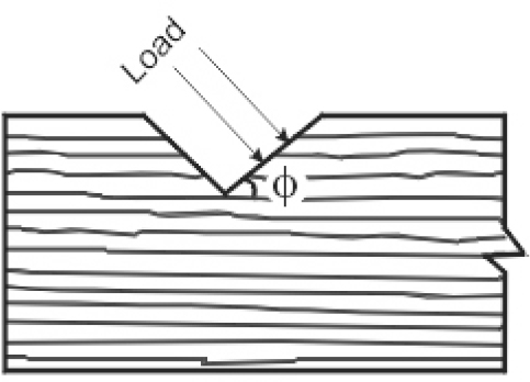
Inclination of load on timber grains
When the direction of stress is at an angle to the direction of grain in any structural member, as shown in Figure 9.12, the permissible bearing stress in that member is calculated from Hankinson’s formula. According to this formula,
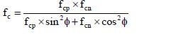
| Here, | fc | =Permissible compressive stress in the direction of the line of action of the load |
| fcp | =Permissible compressive stress parallel to the grains | |
| fcn | =Permissible compressive stress normal to the grains | |
| ϕ | =Angle of load with respect to the direction of grains |
Design of columns
In general, the timber column is composed of a single piece of wood. The cross section adopted is normally rectangular or circular. Timber columns can be classified as short, intermediate and long on the basis of the slenderness ratio, which in this case is considered as the ratio of unsupported length to the least side of the cross-sectional area.
If the unsupported length is l and least sectional dimension is d, the following classification shall be applicable.
Short Column – If l /d ≤ 11
In the case of short columns, the permissible stress in the section would be the allowable stress in compression for the timber.
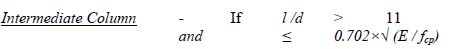
Here, E = Modulus of Elasticity for the Timber
In this case, the permissible compressive stress is calculated from the following relation:

Long Column – If l /d > 0.702×√ (E / fcp)
In the case of long columns, the following formula provides the value of the permissible compressive stress in the section:
fc = 0.329 E / (l/d)2
We will see the illustration below to fully understand the procedure.
Illustration 9.1: A timber column has a section of 200 mm × 200 mm and unsupported length of 2.5 m. The force has been acting along the grains. The objective is to determine the maximum permissible compressive load on the column.
The design data are given as follows:
| Max permissible compressive stress | = 5.5 N/mm2 |
| Modulus of elasticity | = 10650 N/mm2 |
| The slenderness ratio for the column = | 2.5 × 1000 / 200 = 12.5 |
Since the slenderness ratio is more than 12.5, the column is definitely not a short column.
| The value of | K | = | 0.702×√ (E / fcp) |
| = | 0.702×√ (10650 / 5.5) | ||
| = | 30.89 |
Since the slenderness ratio is less than 30.89 (value of K), this is an intermediate column. The permissible compressive stress in this column,
| fc | = | fcp× [ 1 – l4 / 3 (K×d)4] |
| = | 5.5× [ 1 – (2500)4 / 3 (30.89×200)4] | |
| = | 5.45 N/mm2 |
Therefore, the maximum permissible load in the column,
| P | = | 5.45 × 2002 |
| = | 218000 N | |
| = | 218 kN |
Design of beams
In the case of timber beams, usually a single piece of rectangular cross section is used. If the span is too large or the load is too high, it is possible to form a built-up section by bolting or spiking smaller cross-sectional wooden piece together.
The design of a wooden beam is conceptually similar to steel beams. However, if the depth of the rectangular beam is in excess of 300 mm, following form factor is applied to the permissible bending stress:

The other part of the process of design of timber beam is identical to the process for any other homogeneous material.
9.6 Conclusion
In this chapter, we went through the concept of design of masonry structures, common masonry constructions and their features. It has to be remembered that masonry is one of the important construction materials, and knowledge about its design is essential for any structural engineer.
In the second part of the section, we studied in detail the characteristics of timber which influence its use as a structural material. The diversity within wood is very large and it was not possible to cover all kinds of wood with their characteristics, but a general overview has been presented and, with this, it is possible to understand the benefits and limitations of a timber structure.
In the end, some design fundamentals for timber structures have been covered. It was not the objective to cover the design aspect comprehensively but to provide an idea to the reader about the basics of timber design and the treatment of stresses within it. The important point is that though timber is like any other homogeneous construction material, it requires special attention due to some of its inherent properties, especially at high stress.
Compiled by:
C. Scheffer
2003
Exercise A – Static determinacy
1. Classify each of the beams shown below as statically determinate or statically indeterminate. If statically indeterminate, report the number of degrees of indeterminacy. All beams are subjected to external loadings that are assumed to be known and can act anywhere on the beams.
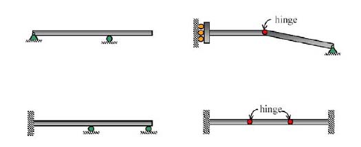
2. Classify each of the pin-connected structures shown in the figure below as statically determinate or statically indeterminate. Report the number of degrees of indeterminacy.
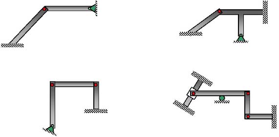
3. Classify each of the frames shown in the figure below as statically determinate or statically indeterminate. If statically indeterminate, report the number of degrees of indeterminacy.
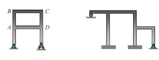
Exercise B – Reaction forces
1. Determine the reactions on the beam shown.
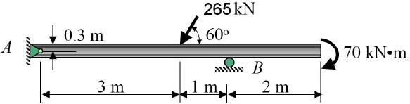
2. Determine the reactions on the beam shown.
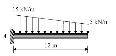
3. The side girder shown in the photograph supports the boat and the deck. An idealized model of this girder is shown in the figure below, where it can be assumed that A is a roller and B is a pin. Using a local code the anticipated deck loading transmitted to the girder is 6 kN/m. Wind exerts a resultant horizontal force of 4 kN as shown, and the mass of the boat that is supported by the girder is 23 Mg. The boat’s mass center is at G. Determine the reactions at the supports.
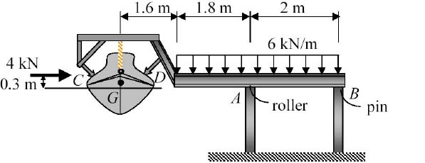
Exercise C – Trusses
1. Classify each of the trusses in the figure below as stable, unstable, statically determinate, or statically indeterminate. The trusses are subjected to arbitrary external loadings that are assumed to be known and can act anywhere on the trusses.
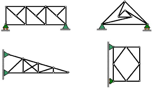
2. Determine the force in members GF and GD of the truss shown in the figure below. State whether the members are in tension or compression. The reactions at the supports have been calculated.
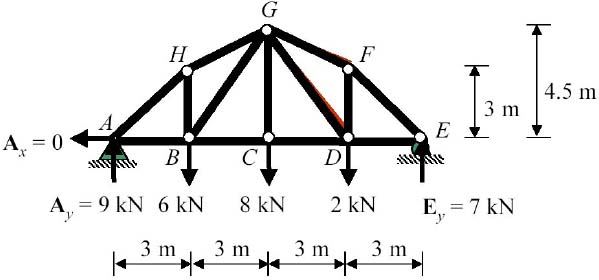
Exercise D – Shear force and bending moment diagram
Plot the shear force and bending moment diagrams for the beam shown below.
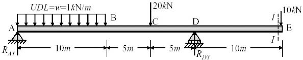
Exercise E – Influence lines
Construct the influence line for:
- the reaction at A, C and E
- the shear at D
- the moment at D
- shear before and after support C
- moment at point C
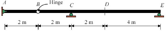
Exercise F – Stress in beams
1. Determine the position of the neutral axis, the second moment of area and the section modulus (around top and bottom) for the cross section of the beam shown below.
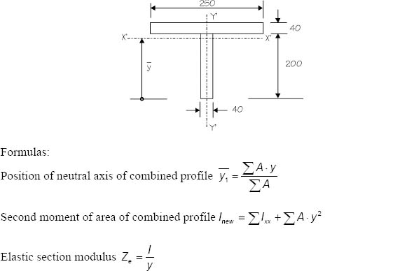
2. Determine the maximum tensile and compressive stress in the beam shown below. The beam properties and the load diagrams are given.
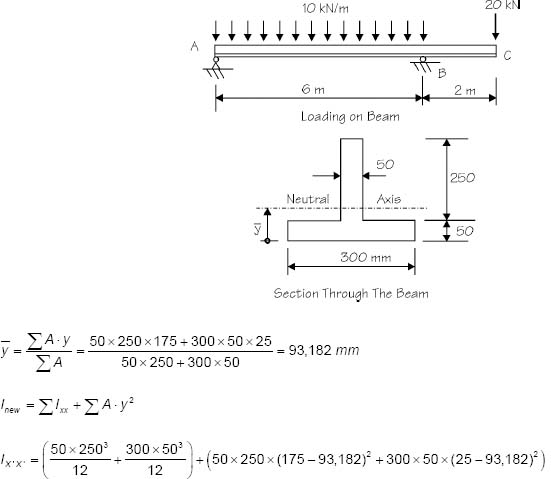
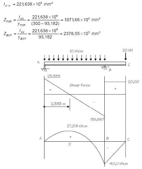
3. Determine the stress under the following concrete wall that works as a dam wall. The density of concrete = 2400 kg/m3 and of the water = 1000 kg/m3. Assume that gravity acceleration, g = 10 m/s2. Use a 1 m length of the wall. The section modulus is  The width b in the equation = 1 m and the height h = 2 m.
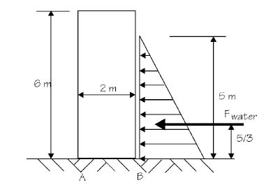
Exercise G – Statically indeterminate structures
1. Determine the bending moment diagram of the following statically indeterminate beam. Use the slope deflection method.
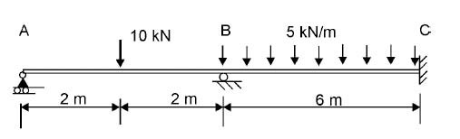
2. A beam rests on a solid rock and two springs. Determine the bending moment diagram of the beam if the load is applied and the springs have a stiffness of 1 kN/mm. The beam has the following properties: I = 100 x 10-6 m4; E = 200 GPa.
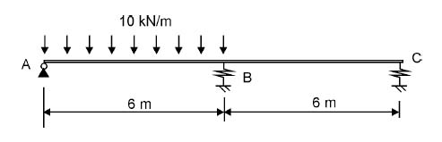
Exercise H – Design theories and loads
1. A mild steel cable with a characteristic yield stress of Sy = 250MPa has to support a self-weight load of 3kN and an imposed load of 2kN. Find the required cross-sectional area for the rope based on the following methods:
a) Load factor method using a load factor of 1.8
b) Allowable stress method using a safety factor of 1.8
c) Limit state method using partial safety factors of:
- 1.2 for self-weight (dead load)
- 1.6 for imposed (live) load
- 1.15 for steel
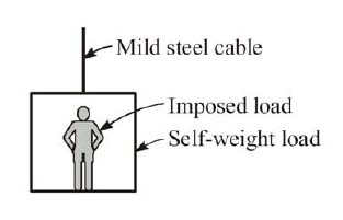
2. A beam is supported by two foundations A and B and is subjected to a live load of Qn = 170kN at point C. The unit weight of concrete is 24kN/m3. The dimensions of the beam are:
L1 = 6m b = 0.6m
L2 = 2m h = 1.4m
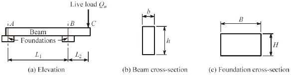
a) Determine the required weight of the foundation at A that will prevent uplift (apply a partial load factor of 1.6 to the live load, 0.9 to the self-weight between AB and 1.2 to the self-weight between BC).
b) The same foundation is to be provided at A and B. Each foundation is in square plane with B = 2 m and has a depth of H = 1 m. Determine the maximum bearing pressure on each foundation (apply a partial load factor of 1.6 to the live load and 1.2 to the self-weight throughout).
Exercise I – Fasteners and welds
1. The figure below shows a ball bearing encased in a “pillow block” supporting one end of a rotating shaft. The shaft applies a static load of 9 kN to the pillow block. Select appropriate metric screw threads for the pillow block attachment and specify an appropriate tightening torque. Use a safety factor of 4 and the given tables for bolts at the end of this exercise.
Initial tightening: Fi = 0.9 At Sp
Tightening torque: T = 0.2 Fi d
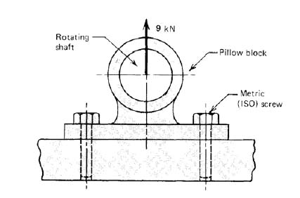
2. Determine the tensile stress in the bolted connection shown below for the load F = 170 kN. Using a safety factor of 4, comment on whether the plates will fail or not if the yield strength of the plate material is 250 MPa. The bolts are M12.
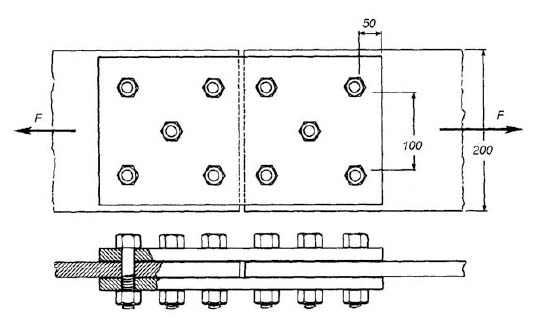
3. The plates in the welded joint shown in the figure below are 12 mm thick and are made of steel having Sy = 350 MPa. They are welded together with convex fillet welds along sides AB and CD, each 50 mm long. The yield strength of the weld material is also 350 MPa. With a safety factor of 3 (based on yield strength), what static load F can be carried using a 6 mm weld leg?
Hint: Distortion energy theory states that Ssy = 0.58 Sy for welds in shear.
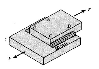
4. Determine the required weld size for the design below using E60 welding rods (Sy = 345MPa) and a safety factor of 2.5 based on yielding. Hint: The maximum stress occurs at point C.
Shear stress = Tr / J
t = weld size
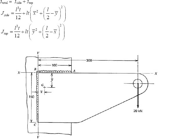
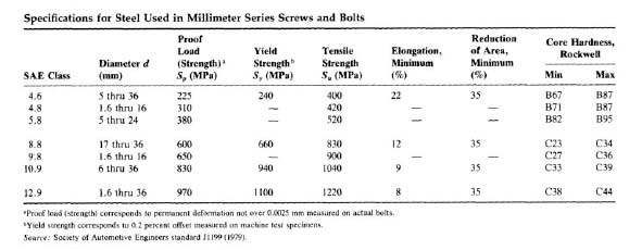
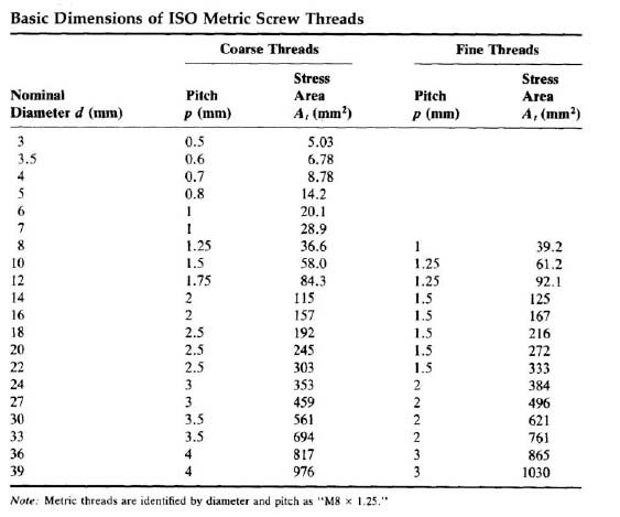
Exercise J – Design of steel elements
1. A steel Universal Column with 254 x 254 x 89 kg/m has a cross-sectional area of 11 400 mm2 and the second moment of area around the minor axis is 48.49 x 106 mm4. If the column has to carry an axial load of 1600 kN and is fixed at its base and pinned at the top, what is the longest length of column that can be used without buckling? The effective buckling length for a fixed-pinned member is le = 0.7 x l.
2. Sketch possible collapse mechanisms for the three-span continuous beam shown in the figure below.
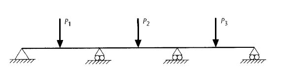
3. A propped cantilever of 4 m length and plastic moment capacity of 150 kN/m carries a concentrated load P at its midspan. Find the value of P that will cause collapse.
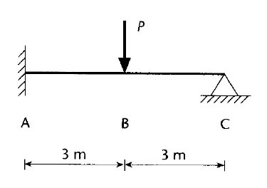
Exercise K – Design of RCC structures
1. Which factors influence the shrinkage of concrete?
2. Which factors influence the creep of concrete?
3. A 220 mm wide beam is simply supported and spans 6 m. Assume a bar diameter of 25 mm, stirrup = 12 mm and a cover of 25 mm. Calculate the percentage of steel required if the beam carries the following loads:
- Dead Load (DL) = 12 kN/m
- Live Load (LL) = 18 kN/m
- Design load wu= 1.2 x DL + 1.6 x LL
Use the following properties:
- Concrete stress, fcu = 30 MPa
- Reinforcing stress, fy = 450 MPa
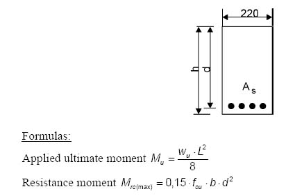
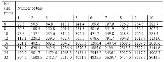
Tip: Set the applied ultimate moment = the resistance moment, then solve d and round off h to nearest 25 mm. Calculate practical d and solve Mu.
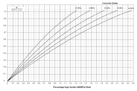
Exercise L – Limit state design of timber structures
A. Partial material factors
The following partial material factors are used to modify the characteristic stresses. These factors are unique to timber and reflect the strength of timber to factors such as the duration of the load, moisture variation, etc.
1. Partial material factor for load duration, γm1
Timber is susceptible to cumulative damage. The longer a load is applied the more the damage. When loads are of short duration, the members have a higher capacity for load and the γm1 factor can be used to reflect this higher capacity. The factor for duration of load is given by
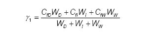
WD = effect of permanent load
WI = effect of imposed load
WD = effect of wind load
CfD = factor of permanent load
CfI = factor for imposed load
CfW = factor for wind load
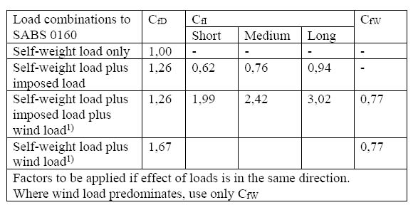
2. Partial material factor for load sharing, γm2
This factor should not be applied to members of structural systems that have similar stiffness and does not display a ductile failure mode, such as laminated beams.
3. Partial material factor for stressed volume, γm3
Some specified strength of members vary with member size and applied loading, and these should be modified by a volume factor γm3.
All the characteristic stresses of truss members should be modified by
γm3 = 0.87 + 0.015 L
For girders and beams
γm3 = 0.85 + 0.03 L
where L is the span (distance between supports) measured in metres.
4. Partial material factor for moisture content, γm4
The strength of compression members is influenced by the moisture content and if the moisture content increases above a value of 17%, the strength of the member may decrease. If the moisture content regularly exceeds 20%, the value of γm4 should be taken as 1.33. In all other cases use a value of 1.0.
5. Partial material factor for pressure treatment, γm5
Where members have been pressure-treated with water-borne preservatives or fire retardants that damage the timber, the specified strengths and resistances shall be modified by a treatment factor, γm5, equal to 1.11.
B. Design Code for tension members:
For a safe design SABS 0163 requires us to ensure that the tensile resistance is greater than the tensile force induced by external loads. All holes greater than 6 mm in diameter must be deducted from the area:
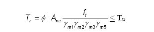
Tr = tensile resistance
Tu = the applied factored tensile load
Ane = net area
ft = characteristic tensile stress
φ = capacity reduction factor = 0.68
Table N1: Characteristic stresses for South African Timber (MPa).
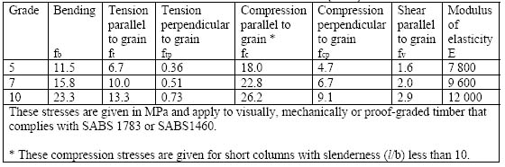
1. Calculate the maximum factored load that may be applied to a 38 x 154 Saligna (grade 10) board if a 20 mm hole is drilled through it. The board is used in tension parallel to the grain. Use a permanent load effect of 2.4 and an imposed load effect of 1.6.
2. A tension member in a truss is subjected to a load of 40 kN. The load is made up of a permanent component of 22 kN and an imposed load component of 18 kN. Use a grade 10 Saligna and determine a suitable member size, and use a permanent load effect of 1.2 and an imposed load effect of 1.6.
3. Determine the tensile resistance of a grade 5, 36 x 111 tension member with a 22 mm bolthole. The product of the material factors γm1…γm5 = 0,85.
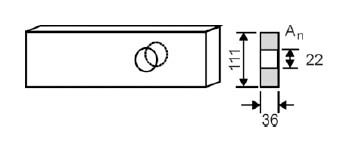

Professional Certificate of Competency in Advanced TCP/IP-Based Industrial Networking
Designed for engineers and technicians who need practical knowledge in…Read more
Professional Certificate of Competency in Allen Bradley Controllogix / Logix5000 PLC Platforms
Designed for engineers and technicians who need practical knowledge in…Read more
Professional Certificate of Competency in Arc Flash Protection
Designed for engineers and technicians who work in the electrical…Read more
Professional Certificate of Competency in Chemical Engineering and Plant Design
Designed for engineers and technicians who need practical knowledge in…Read more
Professional Certificate of Competency in Circuit Breakers, Switchgear and Power Transformers
Designed for engineers and technicians who need practical knowledge regarding…Read more
Professional Certificate of Competency in Control Valve Sizing, Selection and Maintenance
Designed for engineers and technicians who need a solid understanding…Read more
Professional Certificate of Competency in Electrical Power System Fundamentals for Non Electrical Engineers
Designed for engineers and technicians who need to understand the…Read more
Professional Certificate of Competency in Electrical Power System Protection
Designed for engineers and technicians who need practical skills and…Read more")
Professional Certificate of Competency in Electrical Wiring Standards: AS/NZS 3000:2018 (Australia and New Zealand Only)
This professional development course is designed for engineers and technicians…Read more
Professional Certificate of Competency in Fundamental E & I Engineering for Oil and Gas Facilities
Designed for engineers and technicians who need to update their…Read more
Professional Certificate of Competency in Gas Turbine Engineering
Designed for engineers and technicians who need practical skills in…Read more
Professional Certificate of Competency in Hazardous Areas and Intrinsic Safety For Engineers and Technicians
Designed for engineers and technicians who need to understand the…Read more")
Professional Certificate of Competency in Heating, Ventilation and Air-Conditioning (HVAC)
Designed for engineers and technicians from a wide range of…Read more
Professional Certificate of Competency in IEC 61850 Based Substation Automation
Designed for engineers and technicians who need to understand the…Read more
Professional Certificate of Competency in Industrial Data Communications
Designed for engineers and technicians who need to understand how…Read more
Professional Certificate of Competency in Instrumentation, Automation and Process Control
Designed for engineers and technicians who need to gain practical…Read more
Professional Certificate of Competency in Machine Learning and Artificial Intelligence
This professional development course is designed for engineers and technicians…Read more
Professional Certificate of Competency in Mechanical Engineering
This professional development course is designed for engineers and technicians…Read more
Professional Certificate of Competency in Onshore and Offshore Pipeline Systems
Designed for engineers and technicians who need to gain an…Read more
Professional Certificate of Competency in Power Distribution
designed for engineers and technicians who need to gain a…Read more
Professional Certificate of Competency in Practical Machine Learning Using Python for Engineers and Technicians
Designed to use Python Programming to work with machine learning…Read more
Professional Certificate of Competency in Practical Python for Engineers and Technicians
Designed for engineers and technicians who need to understand the…Read more & SCADA Systems")
Professional Certificate of Competency in Programmable Logic Controllers (PLCs) & SCADA Systems
Designed for engineers and technicians who need to get practical…Read more
Professional Certificate of Competency in Project Management for Engineers & Technicians
This professional development course is designed for engineers and technicians…Read more
Professional Certificate of Competency in Safety Instrumentation Systems for Process Industries
Professional development course designed for engineers and technicians who want…Read more
Professional Certificate of Competency in Sewage and Effluent Treatment Technologies
Designed for engineers and technicians who need practical skills and…Read more
Professional Certificate of Competency in Structural Design for Non Structural Engineers
Professional development course designed for engineers and technicians who need…Read more")
Professional Certificate of Competency in Substation Design (Main Equipment)
Professional development course is designed for engineers and technicians who…Read more")
Professional Certificate of Competency in Substation Design (Control, Protection and Facility Planning)
Designed for engineers and technicians who need to gain practical…Read more
Professional Certificate of Competency in the Fundamentals of Process Plant Layout & Piping Design
Professional development course is designed for engineers and technicians who…Read more
Professional Certificate of Competency in Practical Mechanical Sealing
This professional development course is designed for engineers and technicians…Read more
Professional Certificate of Competency in Road Construction
This professional development course is designed for engineers and technicians…Read more
Professional Certificate of Competency in Specification and Technical Writing
Master the art of writing clear, accurate, and professional technical…Read more
Professional Certificate of Competency in Hydraulics and Pneumatics
Overview of all aspects related to the construction, design, operation,…Read more
Professional Certificate of Competency in Big Data and Analytics in Electricity Grids
This course explores the use of big data & data…Read more
Professional Certificate of Competency in Renewable Energy Systems
This course covers various renewable energy systems that are popular…Read more
Professional Certificate of Competency in Smart Grids
A smart grid is an electricity network that uses digital…Read more
Professional Certificate of Competency in Hydrogen Energy – Production, Delivery, Storage and Use
Hydrogen energy short course designed for engineers and professionals interested…Read more")
Professional Certificate of Competency in Building Information Modelling (BIM)
This professional development course is covering practical aspects of using…Read more
Professional Certificate of Competency in Industrial Internet of Things
Internet of Things (IoT) is the most sort after technology…Read more