This technical manual covers the practical aspects of pipeline design, integrity, maintenance and repair, including the applicable codes and standards, with a focus in a land-based environment.
IDC Technologies Pty Ltd
PO Box 1093, West Perth, Western Australia 6872
Offices in Australia, New Zealand, Singapore, United Kingdom, Ireland, Malaysia, Poland, United States of America, Canada, South Africa and India
All rights to this publication, associated software and workshop are reserved. No part of this publication may be reproduced, stored in a retrieval system or transmitted in any form or by any means electronic, mechanical, photocopying, recording or otherwise without the prior written permission of the publisher. All enquiries should be made to the publisher at the address above.
ISBN: 978-1-921007-00-2
Disclaimer
Whilst all reasonable care has been taken to ensure that the descriptions, opinions, programs, listings, software and diagrams are accurate and workable, IDC Technologies do not accept any legal responsibility or liability to any person, organization or other entity for any direct loss, consequential loss or damage, however caused, that may be suffered as a result of the use of this publication or the associated workshop and software.
In case of any uncertainty, we recommend that you contact IDC Technologies for clarification or assistance.
Trademarks
All terms used in this publication that are believed to be registered trademarks or trademarks are listed below:
Acknowledgements
IDC Technologies expresses its sincere thanks to all those engineers and technicians on our training workshops who freely made available their expertise in preparing this manual.
Contents
1 Introduction and Overview 1
1.1 Pipeline Basics and Factors Influencing Pipeline Design 1
1.2 Pipeline Route Selection 3
1.3 Codes and Standards Affecting Pipeline Design, Construction, Operation and Maintenance 4
1.4 Pipeline Design Principles- Hydraulics, Mechanical Design and Materials of Construction 5
1.5 Pipeline Construction Fundamentals 5
1.6 Pipeline Protection and Maintenance 6
1.7 Pipeline Economics 7
1.8 Physical Quantities and Units used in Pipeline Design 8
1.9 Case Study 10
1.10 Summary 20
2 Pipeline Design, Operation and Maintenance Standards 23
2.1 Codes and Specifications 23
2.2 List of Organizations involved in the Generation and Publication of Pipeline Codes and Standards 24
2.3 Major Codes and Standards Governing the Design, operation and Maintenance of Pipeline 24
2.4 Development of Codes and Standards 26
2.5 Common Features of Pipeline Codes and Standards 26
2.6 Features of ASME B31.4: Pipeline Transportation Systems for Liquid Hydrocarbon and Other Liquids 28
2.7 Features of AS2885 (Australian Standard 2885): Pipelines – Gas and Liquid Petroleum 28
2.8 Symbols and units used in Pipeline Design Standards 32
2.9 Abbreviation Used in Pipeline Design Standards 33
2.10 Information Typically Contained in Piping Specifications 34
2.11 Standards and Guidelines for Pipeline Operations and Maintenance 35
2.12 Summary 36
3 Pipeline Routing 37
3.1 Introduction to Pipeline Routing 37
3.2 Factors Influencing Pipeline Routing 38
3.3 Acquisition of Land for Pipeline Construction 39
3.4 Pipeline Routing Thumb Rules 39
3.5 Tools Used in Pipeline Routing 40
3.6 Data Used in Pipeline Routing 40
3.7 Consideration of Alternate Routes 41
3.8 Route Selection Case Study 42
3.9 Summary 44
4 Pipeline Hydraulics- Fluid Properties 47
4.1 Fluid Properties and their units 47
4.2 Summary 51
5 Liquid Flow and Pumps 53
5.1 Fundamentals of Liquid Flow: Continuity Equation 53
5.2 Laminar Flow of Liquids 55
5.3 Turbulent Flow of Liquids 57
5.4 Pump Basics and Types of Pumps 60
5.5 Centrifugal Pumps 61
5.6 Reciprocating Pumps 61
5.7 Pump Drivers 62
5.8 Pump Performance Parameters 62
5.9 Pump Calculations: Power Requirements 64
5.10 Pump Calculations: Affinity laws 64
5.11 Pump Cavitation 65
5.12 Changing Pump Parameters to Meet Fluctuations in Pipeline Operating Conditions 66
5.13 Net Positive Section Head (NPSH) 66
5.14 Optimization of Line Size, Pressure Drop and Location of Pumping Stations 67
5.15 Summary 68
6 Gas Flow and Compressors 69
6.1 Calculation of Gas Densities 69
6.2 Continuity Equation for Gas Flow 71
6.3 Compressible Flow of Gases 71
6.4 Reynolds Number and Friction Factor for Gas Flow 72
6.5 Equations for Gas Flow Through Pipelines 73
6.6 Gas Compressors 77
6.7 Types of Gas Compressors and Drivers 77
6.8 Selection of Gas Compressors 78
6.9 Isothermal Gas Compression 79
6.10 Reversible Adiabatic or Isentropic Gas Compression 80
6.11 Power Required for Gas Compression 81
6.12 Additional Gas Compression Equations for Isentropic Compression 81
6.13 Guidelines for Compressor Design and Selection 82
6.14 Design Optimization of Gas Pipeline 83
6.15 Compressor Stations 84
6.16 Summary 85
7 Mechanical Design of Pipelines 87
7.1 Forces and Stresses in Pipelines 87
7.2 Introduction to Mechanical Design 88
7.3 Mechanical Design Parameters 88
7.4 Criteria for Mechanical Design including Code Criteria 88
7.5 Specified Minimum Yield Strength of Pipeline Materials 89
7.6 Mechanical Design Equations: Calculations of Maximum Allowable Pressure (MAP) and Minimum Required Wall Thickness of Pipelines 90
7.7 Sustained Loads in Pipelines 92
7.8 Thermal Expansion/ Contraction of Materials 93
7.9 Stresses Due to Thermal Expansion/ Contraction 93
7.10 Quick Estimate of Weight of Pipeline 95
7.11 Estimating the Maximum Span of Unsupported Pipe 95
7.12 Estimating Expansion/ Contraction of Pipeline 96
7.13 Case Study 96
7.14 Summary 98
8 Pipeline Construction 99
8.1 Introduction 99
8.2 Sequence of Construction Activities 100
8.3 Construction Equipment 100
8.4 Preparing of the Right of Way (ROW) for the Pipeline 103
8.5 Stringing the Pipeline 104
8.6 Bending 104
8.7 Welding and Post-Weld Qualification 104
8.8 Lowering 105
8.9 Tie-in and Assembly 105
8.10 Testing and Inspection 105
8.11 Back Filling of Trench 105
8.12 Construction Techniques Used in Water Crossing 106
8.13 Commissioning the Pipeline 107
8.14 Cleaning and Restoration 107
8.15 Case Study 108
8.16 Summary 109
9 Pipeline Protection and Maintenance 111
9.1 Possible Causes of Pipeline Damage 111
9.2 Consequences of Pipelines Damage 112
9.3 Prevention of Pipeline Damage 112
9.4 Characteristics and Properties of Pipeline Coatings 113
9.5 Corrosion Fundamentals 113
9.6 Cathodic Protection 114
9.7 Internal Corrosion 117
9.8 Stress Corrosion Cracking (SCC) 117
9.9 Pipeline Integrity Programs 117
9.10 Case Study 119
9.11 Summary 122
10 Pipeline Economics and Asset Management 123
10.1 Introduction to Pipeline Economics 123
10.2 Terminology Used in Pipeline Economics 124
10.3 Case Study 125
10.4 Pipeline Performance: Key Performance Indicators (KPIs) for Monitoring and Assessing Pipeline Performance 127
10.5 Summary 130
A Appendices 131
Solutions to Practical Exercises
B Appendices 167
Article
This chapter provides an introduction to the course and also a brief overview of the course topics. The objective of this chapter is to set the framework for the course and provide the reader with a good feel of the topics covered in the course.
Learning objectives
Fundamental aspects of the following topics:
Pipeline Basics and factors influencing Pipeline Design.
Pipeline Route Selection.
Codes and Standards Affecting Pipeline Design, Construction, Operations and Maintenance.
Pipeline Design Principles: Hydraulics, Mechanical Design and Materials Selection.
Pipeline Construction Fundamentals.
Pipeline Protection and Maintenance.
Pipeline Economics.
Physical Quantities and Units used in Pipeline Design.
Practical Exercises.
Comprehensive Case Study illustrating different aspects of pipeline design, operations and maintenance.
1.1 Pipeline Basics and Factors Influencing Pipeline Design
Pipelines play a vital role in the transmission of oil and gas from the source to the destination for further refining, processing and storage. Most of developed countries have an extensive pipeline network that help meet energy and product demands at different locations. Pipeline construction and use is increasing at a rapid pace in developing nations. Pipelines traverse large distances and can be above ground or below ground. Pipelines also cross bodies of water such as lakes and rivers. A picture of the Trans-Alaska pipeline is shown in Figure 1.1.
Figure 1.1 Trans-Alaska Pipeline
Facts on some well-known pipelines are presented in Table 1.1
Table 1.1
Facts on Some Well-Known Pipelines
Pipeline
Trans-Alaska
Baku-Tbilisi-Ceyhan (BTC)
West-East Gas
Location
Prudhoe Bay to Valdez
Caspian Sea to Mediterranean Sea
Xingjiang Uygur to Shanghai
Commodity
Crude Oil
Crude Oil
Natural Gas
Length
800 miles
1100 miles
2500 miles
Constr. Dates
1974 – 1977
2003 – 2005
2002 – 2004
Cost
$7.7 billion
$3.6 billion
$5.2 billion
Features
Extreme Terrain and Climate, Permafrost, Environment
Traverses mountain ranges, roads, railways, water bodies
Traverses three mountains, 37 rivers. Used remote sensing technology.
Status
2 million BPD at peak (1988). 890,000 BPD in 2005
150,000 BPD in June 2005. Will reduce by 350, the tankers through Bosphorus Strait
1.3 billion cubic meters of natural gas in 2004, its first year of operation
The design, construction, maintenance and operation of pipeline involve the use of several engineering, scientific and economic principles. The location of the pipeline depends on the location of the source of the commodity and its destination. The routing of the pipeline involves consideration of factors such as the terrain, topography, climate and the environment. Construction techniques are adopted to suit the terrain, the soil and the environment. Compressor stations support the operation of gas transmission lines and pumping stations support pipelines transporting liquids.
The major factors influencing the design and construction of pipelines are listed here.
Nature of fluid being transported (gas or liquid) and fluid properties.
Volume flow rate.
Length of the pipeline.
Terrain and medium (soil/water) traversed by the pipeline.
Climatic conditions – extreme heat/cold.
Environmental constraints and impact on the environment.
Codes, standards and regulations governing the design, construction and operation of the pipeline.
Seismic/volcanic conditions.
Flood plains and potential for flooding.
Economics.
Materials.
Construction, operation and maintenance of the pipeline.
The objective of pipeline design and engineering is to route, design and construct a pipeline that can operate safely with minimal impact on the environment and one that is cost effective both in terms of capital and operating costs. To achieve this objective, sophisticated engineering and economic studies are necessary to optimize variables such as pipeline routing, size (diameter), materials and compression/pumping requirements.
1.2 Pipeline Route Selection
The pipeline is routed to connect the supply and delivery points in an optimal, cost-effective manner keeping in mind the operational costs as well as the environmental impacts. The factors that influence pipeline routing are listed here.
Location of supply and delivery points.
Terrain and vegetation.
Location of control points such as river crossings, mountain passes and densely populated areas.
Location and nature of flood plains – usually pipelines should operate continuously under 1:50 year flood conditions and should not sustain major damage from a 1:100 year flood.
Construction access and constructability issues such as the ease with which construction equipment can be moved in and out of suggested routing.
Requirements and location of maintenance facilities such as pig launching and receiving stations.
Pipeline routing is an iterative process. The shortest route may not be the most cost effective. Engineering and design studies of the proposed alternative routes will have to be under taken to optimize conflicting variables. After a preliminary routing is established, it is assessed with respect to the factors mentioned earlier. Some of the tools and techniques used in the assessment of the preliminary routing are listed here.
Geographical Information Systems (GIS).
Detailed Surveying and its results.
Land and soil data.
Hydrological data (riverbed depth and flooding).
Aerial reconnaissance and photographs.
Satellite imaging and data.
Site visits.
Environmental impact studies and their findings.
The preliminary routing is refined and adjusted as necessary based on the results of the route assessment studies.
1.3 Codes and Standards Affecting Pipeline Design, Construction, Operation and Maintenance
Several codes and standards have been developed as guidelines for the design, construction and operation of pipelines. The objective of these codes and standards is to ensure the safety of the personnel and the general public by minimizing the risks of high-pressure pipelines. In addition to codes and standards, pipelines must follow governmental regulations at different levels – federal, state (provincial) and local. Some of the international codes and standards that affect pipeline design, construction and operation are listed here. In some cases a brief description is also provided.
ASME B 31.8 – Gas Transmission and Distribution Piping Systems: This Code covers the design, fabrication, installation, inspection, and testing of pipeline facilities used for the transportation of gas. This Code also covers safety aspects of the operation and maintenance of those facilities.
ASME B 31.4 – Pipeline Transportation Systems for Liquid Hydrocarbons and other Liquids: This Code prescribes requirements for the design, materials, construction, assembly, inspection, and testing of piping transporting liquids such as crude oil, condensate, natural gasoline, natural gas liquids, liquefied petroleum gas, carbon dioxide, liquid alcohol, liquid anhydrous ammonia and liquid petroleum products between producers’ lease facilities, tank farms, natural gas processing plants, refineries, stations, ammonia plants, terminals (marine, rail and truck) and other delivery and receiving points.
AS 2885 – Australian Standard 2885 “Pipelines – Gas and Liquid petroleum.”
This code combines the features of many international and national standards including ASME B31.8, CSA Z662, ISO 13623, API 1104, and ISO 13847.
It has explicit requirements for the design, documentation, and approval of key processes such as prevention of external interference, control of fracture, and welding procedure qualification.
It uses an integral risk assessment and threat mitigation process in design and in operation and maintenance.
It adopts the requirements to suit the specific needs of Australian conditions of longer distances, terrain and population densities
API 5L – API (American Petroleum Institute) Specifications for Line Pipe: Covers welded and seamless pipe suitable for use in conveying gas, water, oil in both the oil and natural gas industries.
API 6D – Specifications for Pipeline Valves, End Closures, Connectors and Swivels: API 6D is the primary standard for valves used in pipeline service, including gate, plug, ball and check valves. This standard has more stringent testing requirements.
API 1104 – Welding of Pipeline and Related Facilities.
ASTM A106 – Seamless Carbon Steel Pipe for High Temperature Service.
NACE RP-01-92 – Control of External Corrosion on Underground or Submerged Piping System.
ISO 9001 – Quality Systems for Design/Development, Production, Installation and Servicing.
API RP 5L2 – Recommended Practice for Internal Coating of Line Pipe for Gas Transmission Service.
1.4 Pipeline Design Principles – Hydraulics, Mechanical Design and Materials of Construction
The design and detailed engineering of pipelines requires the knowledge and application of fluid mechanics (hydraulics), stress analysis and materials science.
The temperature and pressure of the fluid flowing in the pipeline are important parameters that affect the fluid properties as well as the wall thickness and the insulation requirements.
Principles of fluid mechanics are used in the calculation of friction losses, pressure drop, and pumping requirements. Additionally, they are also used in the measurement and metering of flow through the pipelines.
Pipelines are subjected to forces resulting from internal pressure as well as other factors such as wind, thermal expansion, displacements, seismic movements and soil loads. These forces create stresses in the pipeline walls. The mechanical design of pipelines uses the principles of stress analysis to calculate stresses within the pipeline and to ensure that they are well within the allowable limits specified by the codes.
The subject matter of thermodynamics covers topics related to principles of gas compression, pressure – temperature relationships for gas compression, energy and Power requirements for pumps and compressors.
The nature of the commodity flowing in the pipeline and the surrounding environment (soil, water or above ground) determine the material to be used in the pipeline. Different grades of steel can be used depending on cost, wall thickness, welding requirements and toughness. The subject matter of materials science covers the topics related to: selection of appropriate materials for pipeline systems including pipe, valves, fittings, flanges, pumps and compressors, selection of appropriate insulation materials, principles of corrosion, techniques to minimize corrosion including cathodic protection.
1.5 Pipeline Construction Fundamentals
The techniques used in the construction of pipelines depend on the nature of the route traversed by the pipeline – above ground or below ground, the terrain, and crossing of bodies of water, if any. Also, construction techniques are dependant on the season – techniques that are effective during summer may not be appropriate during winter. Construction operations and activities must comply with the regulations in effect along the pipeline route. Most of these regulations are intended to protect the environment and to promote public safety. Regulatory agencies conduct inspections to ensure compliance. Restoration of the environment to pre-construction status constitutes an important part of construction activities. The optimization of construction costs takes place during the route selection process. Common procedures and operations used during the construction process are listed here.
Construction Surveying.
Trenching (if below ground).
Clearing and grading the pipeline path (Right Of Way – ROW).
Placing the pipe spools on the ROW.
Stringing the pipe.
Bending.
Welding.
Inspection of pipeline and welds using Non Destructive Testing (NDT) methods.
Backfilling of trenches and restoring the site and the environment (re-vegetation).
1.6 Pipeline Protection and Maintenance
Pipelines are valuable assets that need to be protected and maintained for optimum performance. The primary issue of concern for buried pipelines is external corrosion due to the surrounding soil. The common methods of protecting buried pipelines are external coating and cathodic protection. External coatings are plastic materials placed on the exterior of the pipe using one of the following methods – wrapping, extrusion or fusion bonding. External coatings not only serve as barriers for corrosion attack but also prevent damage to pipeline during transportation, handling and backfilling. Insulation, rock shield and concrete are also used as external coatings. Cathodic protection involves the use of a sacrificial anode or an impressed current that makes the pipeline the cathode. The method of protection employed depends on the nature and composition of the soil. This is determined by an analysis of the soil. During the design phase, the different types of external coatings and cathodic systems are evaluated and an appropriate protection strategy is chosen based on soil conditions and economics.
Corrosive substances, such as sour gas, being transported in the pipeline can also damage pipelines on the inside. The major problem is sulphide stress cracking (hydrogen embrittlement) caused by the presence of hydrogen sulphide (H2S). A better understanding of the corrosion mechanism and the selection of appropriate material that will resist the corrosion will minimize internal corrosion problems.
Despite all the care taken during the design and construction of pipelines, there is always the risk of damage to the pipelines. The damage can be mechanical damage due to other equipment or forces due to soil movement. The damage could also be due to corrosion, mechanical defects and operational factors. This necessitates the monitoring of the pipeline to ensure the structural integrity and the operability of the pipeline. The techniques used in assessing the integrity of pipelines are listed here.
Ultrasonic inspection.
Radiography.
Dye penetration tests.
Magnetic particle testing.
Cathodic protection survey.
Magnetic flux.
Visual inspection.
1.7 Pipeline Economics
The design, engineering and construction of pipelines require significant investment of capital and manpower. Further, the operating expenses of the pipeline also need to be considered. The capital costs and the operating costs are the two principal cost elements in owning and operating a pipeline system. In the initial stages, an economic feasibility study of the pipeline project is required to justify the investment in the pipeline. During such feasibility studies, alternative means of transporting the oil/gas by road or rail will also be considered. The oil/gas can also be fed into an existing line. The alternative that offers the best return on the investment will be chosen. A sample problem involving economic analysis of alternative means of transporting oil is illustrated in Practical Exercise 1.1.
Practical Exercise 1.1
The following data is available on three alternative methods for transporting oil. The cost figures are in millions of dollars. If the transmission company requires a minimum 6% return on investment, which alternative is most economically feasible? Use an analysis period of 30 years for comparison.
Alternative
Initial Investment
Annual Costs
Rail Transport
–
$50M
Lease an Existing Line
–
$60M
New Pipeline
$600M
$5M
Practical Exercise 1.2 illustrates the calculations of return on invested capital and payback period for a pipeline project.
Practical Exercise 1.2
A pipeline project has an estimated capital investment of $600 M. The pipeline will be operational in two years from the start of the construction. Once operational, the pipeline will have projected annual revenue of $105 M for a period of 15 years. Annual operation costs are expected to be $5 M.
Determine:
A. The rate of return for this pipeline project.
B. The pay back period.
Once the feasibility of a pipeline project is proven, further economic analysis is carried out to determine the optimum value of variables such as pipeline diameter, material, wall thickness, routing and pumping/compression requirements. Economics affects almost all design and construction parameters. The results of economic analysis are also used in determining the tariffs to be charged for transmission of commodities through the pipeline.
Further details on the different cost factors and on pipeline economics are presented in Chapter 6.
1.8 Physical Quantities and Units Used in Pipeline Design
The design of pipelines involves engineering and design calculations. It is therefore important to understand the physical quantities (variables) used in pipeline design and engineering calculations.
The key to understanding the physical quantities is to know the definitions of force, pressure and engineering stress.
Definitions of Force: Force is vector quantity that represents mass times acceleration.
The unit of force in the metric system is kilogram force (kgf), which is defined as the force required to accelerate 1 kilogram mass (kgm) at the rate of 9.81m/s2.
The unit of force in the SI system is Newton (N), which is defined as the force required to accelerate 1 kilogram mass (kgm) at the rate of 1m/s2.
The unit of force in the imperial or US Customary System (USCS) is pound force (lbf), which is defined as the force required to accelerate 1 pound mass (lbm) at 32.2 ft/sec2.
Note that subscripts “m” is used for mass units and subscript “f” is used for force units.
Units of Force:
The conversion factors for force units are:
1 kgf = 9.81 N, 1kgf = 2.205 lbf, and 1lbf = 4.4462 N
Pressure:
Pressure is force per unit area and it acts uniformly on the surface.
Units of Pressure: N/m2 (Pascal, Pa),
lbf/in2 (psi), kgf/cm2, bar
Atmospheric pressure at sea level is
101 kPa or 14.7 psia
Commonly used conversion factors for pressure are: 1 bar = 105 N/m2 = 100 kPa
1 lbf/in2 (psi) = 0.0703 kgf/cm2 = 6.896 kPa
Temperature:
Units of Temperature (°F or °C): ° F = 1.8 (°C) + 32, °C = (°F)(5/9) – 32
Absolute temperature: Degree Rankine: °R = 460+ °F, Degree Kelvin: °K = 273 + °C
Mass Flow Rate
Units of mass flow rate (lbm/hr or kgm/s): 1 kgm/s = 132.3 lbm/hr
The mass flow rate will be the same at compressor/pump inlet and outlet as per the law of conservation of mass.
Volume flow rate or liquid/gas throughput:
Units of volume flow rate Liquids: gallons per minute (gpm), Liters per second (L/s), cubic meters per hour (m3/hr), barrels per day (bpd).
Useful conversion factors are:
1 bpd = 0.0066 m3/hr = 0.0292 gpm Gases: The volume of gas depends on the absolute pressure (gage pressure + atmospheric pressure), and absolute temperature of the gas. The volume flow rate of gases is usually specified in terms of Standard Cubic Feet Minute (SCFM – measured at 60°F and 1 atm. Pressure) or Normal cubic meters per hour (nm3/hr – measured at 0°C and 1 atm. Pressure).
1 nm3 = 32.326 SCF and 1 nm3/hr = 0.622 SCFM
Work/Energy:
Work is force times distance.
Units of work: ft-lbf, N.m, kgf.m
Energy has the same units of work.
Units of energy: Btu = 778 ft-lbf, Joule (J = N.m)
Power:
Power is the rate of producing work or consuming energy.
Units of power: HP = 550 ft-lbf/sec, 1 W = 1 J/s,
1 HP = 746 kW
An extensive list of conversion factors for various physical quantities is presented in the Appendix
Unit Prefixes:
kilo (k) = 103
Mega (M) = 106
Giga (G) = 109
milli (m) = 10-3
micro (μ) = 10-6
nano (n) = 10-9
Practical Exercise 1.3
The pressure in a natural gas pipeline is 750 psig and the temperature is 125°F. Calculate:
A. The pressure in kPa and kgf /cm2.
B. The temperature in °C, K and °R
(solution)
Practical Exercise 1.4
The flow of oil in a pipeline is 650,000 barrels per day. Calculate the flow rate in m3/hr and gpm.
(solution)
1.9 Case Study: The Trans-Alaska Pipeline
The Trans-Alaska Pipeline System was designed and constructed to move oil from the North Slope of Alaska to the northern most ice- free port, Valdez, Alaska. The following are some basic facts about the Trans – Alaska Pipeline:
Length: 800 miles.
Diameter: 48 inches.
Crosses three mountain ranges and over 800 rivers and streams.
Cost to build: $8 billion in 1977, largest privately funded construction project at that time.
Construction began on March 27, 1975 and was completed on May 31, 1977.
First oil moved through the pipeline on June 20, 1977.
Over 14 billion barrels have moved through the Trans Alaska Pipeline System.
First tanker to carry crude oil from Valdez: ARCO Juneau, August 1, 1977.
Tankers loaded at Valdez: 16,781 through March 2001.
Storage tanks in Valdez: 18 with total storage capacity of 9.1 million barrels total.
The mission of Alyeska’s Ship Escort Response Vessel System is to safely escort tankers through Prince William Sound.
The Trans – Alaska Pipeline posed several design and engineering challenges, which called for some innovative and creative solutions. A summary of the engineering and design challenges and the methods adopted to overcome them is presented here as an informative and useful case study. The technical details of the Trans – Alaska Pipeline are also presented here along with explanation of basic terminologies associated with pipelines. The reader is strongly urged to review the case study and technical details of the Trans – Alaska Pipeline to obtain a fundamental understanding of pipeline design, engineering, construction, operation and maintenance.
Design and Engineering Challenges: Permafrost
Art Lachenbruch was a geologist at the U.S. Geological Survey (USGS) in Menlo Park, California, when he first heard about the Trans – Alaska Pipeline project. Lachenbruch was an expert in permafrost, the rock-like layer of frozen soil just below the thin, insulated cover of soil and vegetation in Alaska. In December 1970, he released a study in which he explained the damage a hot pipe would inflict upon the permafrost. At a temperature of 158 to 176°F, the oil in the pipe would thaw a cylindrical area 20 to 30 feet in diameter within a decade. The thawing would cause damage not only to the pipe, but also to the landscape. This observation led to the complete redesign of the pipeline.
With 75% of the 800-mile pipeline passing through permafrost terrain, the engineers came up with three principal redesign plans to fit the needs of each particular area. The consortium of oil companies building the pipeline, Alyeska, decided to have 380 miles of buried pipeline. Four hundred and twenty miles would be elevated on supports or pilings. The soil on every inch of the pipeline would be tested to figure out which design worked best.
Buried Pipeline
The buried pipeline used was under one of three categories: Conventional below ground pipe, Special non-refrigerated buried pipe and Special refrigerated buried pipe.
Conventional below ground pipe: The designers determined that the conventional below ground pipe could be used in three types of ground: permanently thawed soils, bedrock, and some areas of permafrost which, when thawed, were considered unlikely to cause damage to the pipe. This permafrost was usually a mixture of sand, gravel and ice. Although the method was conventional, the pipeline was not buried like other oil pipelines, which are generally buried in a ditch at a uniform depth. Instead, in Alaska, depending on soil conditions, the engineers buried the pipes at depths of 8ft. to 16 ft. at most locations, but up to a depth of 49 ft. at one location. The pipe is laid on top of a layer of fine bedding material and covered with prepared gravel padding and soil fill material. Zinc ribbons, which serve as sacrificial anodes to inhibit corrosion of the pipe, are buried alongside the pipeline. The Atigun pipe replacement section, 8.5 miles in length, has four magnesium ribbon sacrificial anodes installed. Electrical currents in the earth’s surface, called “telluric currents” and caused by the same phenomenon that generates the Northern Lights, can be picked up by the pipeline and zinc anodes. The zinc anodes act like grounding rods to safely return these currents back to the earth, reducing the risk of damage to the pipeline.
Special buried pipe (non-refrigerated): In areas of thaw-unstable soils calling for elevated pipeline construction, but where the pipeline had to be buried for highway, animal crossings, or avoidance of rockslides and avalanches, the line was insulated, to protect the permafrost from the heat of the pipeline, and buried.
The conventional buried section of the pipeline, including the special insulated sections, account for 376 miles of the pipelines total length of 800 miles.
Special buried pipe (refrigerated): For four miles of the route, neither the conventional buried method nor the elevated one was possible. At these locations, pipe had to be buried in the permafrost to avoid getting in the way of the highway or animal migration as well as a precaution against rockslides and avalanches. These stretches of pipe have their own refrigeration system. The pipe sits on two six-inch coolant pipes. Refrigerated brine is circulated through these lines, powered by electric motors that are housed in a nearby building, which also contains a heat exchanger that removes the heat from the coolant to the outside air. The brine goes into the ground at 8 to 10 degrees Fahrenheit and comes out at 18 to 21 degrees Fahrenheit, absorbing a significant amount of heat from the oil in the pipeline.
Figure 1.2 Buried, Refrigerated Section of the Trans-Alaska Pipeline
Elevated Pipe
Across 420 miles of the pipeline’s route, where the permafrost was unstable and the pipe could not be buried, the engineers designed Vertical Support Members (VSM). These H-shaped pilings elevate the pipe several feet above the ground. The pipe is placed in a Teflon-coated steel shoe that sits on top of the crossbeam. This allows the pipe to slide sideways as it expands (when it’s hot) and contracts (when it’s cold).
In particularly sensitive areas where the permafrost hovers just above the freezing temperature, the engineers added a passive refrigeration system. At those sites, each VSM was equipped with a pair of tubes that sit inside the VSM and descend into the ground. The tubes are filled with anhydrous ammonia, which absorbs the heat, releases it in to the air and then circulates back into the ground. These 2-inch pipes are called “heat pipes.” Heat is transferred through the walls of the heat pipes to aluminum radiators atop the pipes.
Figure 1.3 Elevated Sections of the Trans-Alaska Pipeline with Vertical Support Members (VSMs)
Technical Details on the Trans Alaska Pipeline
Pipe Dimensions:
Outside diameter: 48 in. (122 cm)
Standard Lengths: 40 ft. and 60 ft.
Wall Thickness: 0.462 in. and 0.562 in.
Pieces required for pipeline: Over 100,000
Steel Grades Used for Pipes:
The steel grades used in the pipeline are given along with the Specified Minimum Yield Strength (SMYS) in parenthesis. Mechanical properties are discussed in greater detail in Chapter 7.
Weight Per linear ft.: 235 lbs. (0.462”); 285 lbs. (0.562”)
Total weight shipped: 550,000 tons (approx.)
Insulation
Thickness on elevated pipeline: 3.75 in.
Thickness on refrigerated below ground pipeline: 3.2 in.
Thickness on under gravel work pad or road: 2 in. to 4 in. (limited areas only)
Line Fill
Definition: The amount of oil in pipeline from PS 1 to Marine terminal.
The line fill is 9,059,057 bbl.
Number of pipe shoes: 39,000 (approx.)
Types and number pipeline valves
Check: 81
Gate: 71
Block: 24
Ball: 1
Total: 177
Thermal expansion
Thermal expansion:
Change in pipe length due to change in crude oil temperature
Tie-in temperature:
Actual pipe temperatures at the time when final welds were made, which joined strings of pipe into a continuous line
Hot position:
Pipe at maximum oil temperature (145° F)
Cold position:
Pipe at minimum steel temperature (-60° F) (pre-startup)
Each 40 ft. length of pipe expands 0.031 inches with each 10°F rise in temperature and contracts the same distance with each 10°F drop in temperature.
Longitudinal expansion of typical 720 ft., straight, above ground segment from minimum tie-in temperature to maximum operating temperature will be 9 inches.
Due to anchoring, the pipeline does not expand lengthwise but shifts laterally on the above ground supports.
Maximum above ground lateral movement:
Tie-in to hot position: 8 ft.
Tie-in to cold position: 4 ft.
Maximum thermal stress: 25,000 psi – where below ground pipeline is fully restrained by the soil, the maximum longitudinal stress due to change in temperature from pipe temperature at tie-in to maximum oil temperature
Above ground sections of the pipeline are built in a zig-zag configuration to allow for expansion or contraction of the pipe because of temperature changes. The design also allows for pipeline movement caused by an earthquake.
Pipeline Operations
Maximum daily throughput: 2.136 million bbl., with 11 pump stations operating.
Rates exceeding 1,440,000 bbl./day use Drag Reduction Agent (DRA) injection.
Fuel required for all operations (fuel oil equivalent): 210,000 gal/day.
Maximum operating Pressure: 1,180 psi
Temperature:
At Pump Station 1: 114 ° F at injection into pipeline
At Terminal: 65 ° F approx.
Total travel time: PS 1 to Valdez: 9 days
Velocity: 3.7 mph.
Weight: 310.9 lb./bbl.
Average Throughput (2002 figures):
1 million bbl./day or 41,705 bbl./hr. or 29,194 gal./min.
Recoverable reserves, at discovery (estimated): 13.7 billion bbl.
Pump Stations (PS)
Number of stations in original design: 12
Number of stations operating as of June 2004 was 6, that is, PS 1, 3, 4, 7and 9;
PS 5 is a relief station
PS 11 is a security site.
There were 8 stations operating at start up (PS 1, 3, 4, 6, 8, 9, 10 and 12).
Pumps
Number of pumps operating at a throughput of 0.999 million bbl./day: 2 operating at PS 1, 3 and 9. PS 4, 7 and 12 have 1 unit operating.
Definitions:
Full head pump:
It is a two-stage pump with both impellers in series. It has one inlet and one outlet.
Half head pump:
It is a two-stage pump with both impellers in parallel. It has two inlets and two outlets. It can handle twice the flow of the full head but only produces half the head (pressure rise).
Capacity of mainline pumps:
Half head configuration: 60,000 gpm each
Full head configuration: 20,000 gpm each
Configuration of Pumps:
Half head configuration: PS 2 and 7
Full head configuration: All other pump stations
PS 12 is configured to operate with either 2 full head or 1 half head pump.
Booster pumps: All pump stations have booster pumps to move oil from the storage tanks to the mainline. (PS 1 has three mainline booster pumps to boost oil pressure.) PS 5 also has injection pumps
Power Generation
Size of Power Plants: Ranges from 1.3 MW at PS 12 to 4.7 MW at PS 6, depending on availability of commercial power, presence of topping unit and/or vapor recovery system.
Stations generating electrical power: All stations.
Stations also purchasing commercial power: PS 8, 9 and 12.
Definition of Topping Unit: A mini-refinery that produces turbine fuel.
Location of Topping Units: PS 6, 8 and 10.
Production capacity of Topping Units: 2,400 avg. bbl./day of low sulphur turbine fuel.
Turbines
Fuel requirements:
Gas fired units: 4.3 mcf/unit/day (avg.)
Liquid fired units: 30,000 gal./unit/day (average, for half head configuration) and 24,000 gal./unit/day (average, for full head configuration)
Reaction Turbine Power Output: 18,700 brake horsepower (half head configuration) and 15,300 brake horsepower (full head configuration)
Pig launching/receiving facilities
Three (at PS 1, 4, and Marine Terminal).
Control system
Basic function: Provides instantaneous monitoring, control of all significant aspects of operation, and pipeline leak detection. Operators in the Operations Control Center (OCC) at the Marine Terminal monitor the system 24 hours a day and control oil movement through the pipeline and loading of tankers.
Location: Computer hardware and controllers’ consoles are located in the Operations Control Center (OCC) at the Marine Terminal.
Points monitored:
Pipeline: 3,047 input points and 352 control points.
Marine Terminal: 1,074 input points and 461 control points.
Remote data acquisition units:
Pipeline: 14 (each Pump Station, plus the North Pole Metering facility and Petro Star Refinery)
Marine Terminal: 24
Metering: 14
Software programming functions:
Data acquisition and control
Alarm and data processing and display
Hydraulic modeling
Leak detection
Historical archiving and reporting
Seismic evaluation
Earthquake Protection
Earthquake magnitude pipeline system designed to withstand:
8.5 Richter Scale (maximum).
Range from 5.5 to 8.5, depending on area.
The instrumentation at field locations consists of accelerometers mounted on concrete pads, which measure strong ground motions in three directions (tri-axial) which are connected to a Digital Strong Motion Accelerograph (DSMA). The DSMA, generally located in the Pump Station control room, processes the signals from the accelerometers in real time and reports alarms and selected data to the central processor at the OCC.
Alyeska’s Earthquake Monitoring System (EMS) consists of sensing and processing instruments at all pump stations south of Atigun Pass and at the Valdez Terminal. A central processing unit at the Operations Control Center (OCC) is linked to the Pipeline and Terminal operator consoles. The EMS is specifically designed to process strong ground motions, to interpolate or extrapolate estimates of earth quake accelerations between the sensing instruments and to prepare a mile-by-mile report comparing the estimated accelerations along the pipeline with the pipeline seismic design criteria.
On November 3, 2002, the pipeline withstood a 7.9 earthquake that was centered along the Denali Fault, in the interior of Alaska, approximately 50 miles west of the pipeline. Estimates indicate that the ground along the fault moved 7 feet horizontally and nearly 2.5 feet vertically. The 7.9 quake was the largest on the Denali Fault since at least 1912 and among the strongest earthquakes recorded in North America in the last 100 years.
Glossary of Terms Used in Pipeline Design, Operations and Maintenance Crude Oil: A fluid made up of various hydrocarbon components, natural gas liquids and fixed gases.
Basic conversions: 1 bbl. = 42 gallons, bbl. per ton = 7.07 Gravity: 29.4° API at 60° F (SG = 0.88)
Block Valve: When closed, the valve can block oil flow in both directions. Block valves include manual gate valves, remote gate valves and station block valves (suction valves and discharge valves).
Station Block Valve: A gate valve installed at the inlet (suction) side and the outlet (discharge) side of the pump station to isolate the pump station from the pipeline in the event of an emergency.
Manual Gate Valve: Block valves that are operated manually. Usually placed in check valve segments periodically to provide more positive isolation than can be provided by check valves.
Remote Gate Valve: A remotely controlled block valve for the primary purpose of protecting segments of the line in the event of a catastrophic pipeline break.
Check Valve: Operates one-way and prevents the reverse flow of oil. Check valves are designed to be held open by flowing oil and to drop closed automatically when oil flow stops or is reversed.
Pressure Relief Valve: A valve designed to open automatically to relieve pressure and keep it below a designated level.
Maximum Allowable Operating Pressure: A rating indicating the maximum pressure at which a pipeline or segment of a pipeline may be operated under regulations in normal conditions. Also called pressure rating.
Suction Pressure: Pressure of the oil as it enters a pump station.
Discharge Pressure: Pressure of the oil as it exits a pump station.
Pressure Spike: A sudden, brief rise in pressure.
Pressure Surge: A pressure spike/excursion moving through the pipeline at sonic velocity, produced by a sudden change in velocity of the moving stream that results from shutting down a pump station or pumping unit, closure of a valve or any other blockage of the moving stream.
DRA (Drag Reduction Agent): A long chain hydrocarbon polymer injected into the oil to reduce the energy loss due to turbulence in the oil.
Linefill: The amount of oil in the pipeline from PS 1 to the Marine Terminal.
Slackline: Oil flow that does not completely fill a pipeline.
Packline: Oil flow that completely fills a pipeline.
Breakout Tank: A tank used to relieve surges in a hazardous liquid pipeline system, or to receive and store hazardous liquid transported by a pipeline for re-injection and continued transportation by pipeline.
Permafrost: Any rock or soil material that has remained below 32°F continuously for two or more years.
Pig: A pig is a mechanical device, which is pushed through the pipeline by the oil. Several types of pigs are used to improve flow characteristics, inspect for dents and wrinkles, inspect for pipeline corrosion, and measure pipeline curvature.
Types of Pigs
Scraper:A pig used for cleaning and flow enhancement. Consists of cone-shaped, polyurethane cups on a central body, which matches the shape of the interior pipe wall. Bumper nose, urethane construction and lightweight prevent damage to check valve clappers.
Deformation: A pig, which measures the diameter of the pipe. Defines changes in pipe diameter caused by dents, ovalities, or pipe bending. Changes are recorded and analyzed by engineers.
Corrosion: A pig, which detects corrosion or pitting in the pipe wall. These pigs may use different technologies to collect and record corrosion data. Ultrasonic Corrosion Pig: Measures and records wall thickness of pipeline using ultra sonic transducers.
Magnetic Corrosion Pig: Detects metal loss in pipe wall by measuring disturbances in a magnetic field.
Curvature: A pig using an inertial navigation system to determine pipeline location, curvature and pipe wall deformation.
Telluric Currents: Electrical currents in the earth’s surface which are caused by the same phenomenon that generates the Northern Lights.
Thermal Expansion: Change in pipe length due to a change in crude oil temperature.
Topping Unit: A mini-refinery that draws crude off the line and produces turbine fuel to power the station.
VLCC: Very Large Crude Carrier, tanker 150,000 to 300,000 dwt.
ULCC: Ultra-Large Crude Carrier, tanker more than 300,000 dwt.
VSM: Vertical Support Member
Ultimate Strength: The stress level at which the pipe will fail/rupture or “break.” The ultimate strength of the steel is determined by testing during the manufacture of the pipe.
Yield Strength: The stress level above which the pipe will yield/bend/stretch.
1.10 Summary
The fundamental aspects of pipeline design, engineering, construction, operation and maintenance have been explained in this chapter. In addition, the following topics have been covered:
Physical Quantities and Units typically used in pipeline design.
Pipeline Economics.
Codes and Standards Affecting Pipeline Design and Operations.
Finally, a comprehensive case study of the Trans – Alaska Pipeline has been presented to illustrate the different aspects of pipeline design. A “Glossary of Terms Used in Pipeline Design, Operations and Maintenance” is also included.
This chapter presents a brief overview of the codes, standards and specifications used in pipeline design, operation and maintenance activities. The features of codes and standards from different countries are described. Typical operations and maintenance activities are listed.
Learning objectives
Codes and Specifications.
Codes governing the design of piping systems.
Development of codes.
Features and scope of codes governing pipeline design.
Comparison of pipeline codes from different countries.
Information contained in piping specifications.
Guidelines for pipeline operations and maintenance.
Conclusions.
2.1 Codes and Specifications
Codes are generally broad in nature and scope and are also referred to as “Design Standards”. Codes provide general guidelines for design. However, codes do not have design procedures and formulas for specific situations. Codes do provide recommended equations to calculate maximum allowable limits for stresses. Every code makes it clear to the user that information in codes cannot substitute rigorous calculations and sound engineering judgment. The role and scope of pipeline codes and typical information contained in them are further elaborated in Section 2.4.
Specifications are more detailed in nature and are developed separately for each project. Specifications include details on materials to be used and also details on dimensions of pipe and fittings.
2.2 List of Organizations Involved in the Generation and Publication of Pipeline Codes and Standards
ANSI
American National Standards Institute
API
American Petroleum Institute
APIA
Australian Pipeline Industry Association
AS
Standards Australia
AS/NZ
Standards Australia/Standards New Zealand
ASME
American Society of Mechanical Engineers
ASTM
American Society for Testing and Materials
BS
British Standards Institution
ISO
International Organization for Standardization
MSS
Manufacturers Standardization Society of the Valve and Fitting Industry, USA
NACE
National Association of Corrosion Engineers, USA
2.3 Major Codes and Standards Governing the Design, Operation and Maintenance of Pipelines
The following are the major codes and standards used in the design, operation and maintenance of pipelines:
ASME B31.4: Pipeline Transportation Systems for Liquid Hydrocarbons and other Liquids.
ASME B31.8: Gas Transmission and Distribution Piping Systems.
ASME B31.8S Managing Systems Integrity of Gas Pipelines.
Standard Z662-94, “Oil and Gas Pipeline Systems”, published in 1994 by the Canadian Standards Association (CSA).
National Energy Board Onshore Pipeline Regulations as per the National Energy Board Act, Canada, June 1989.
AS 2885: Australian Standard 2885 – Pipelines, Gas and Liquid Petroleum.
Recommendations on Transmission and Distribution Practice – IGE/TD/1 Edition 3: 1993 Communication 1530 – “Steel Pipelines for High Pressure Gas Transmission”, published by the Institution of Gas Engineers, UK.
“Guidelines for the Environmental Assessment of Cross-Country Pipelines”, published by the Department of Trade and Industry, UK, 1992 (ISBN No. 0114142866).
Code of Practice for Pipelines Part 2. Pipelines on Land: Design, Construction and Installation: Section 2.8: Steel for Oil and Gas. BS 8010: Section 2.8, published by the British Standards Institution, UK, 1992 (ISBN 0580209962).
DVGW Standards G463 – “Steel Gas Service Mains With an Operating Pressure Exceeding 16 Bar; Construction”, and G466/1 – “Gas Steel Pipeline Systems With an Operating Pressure Exceeding 4 Bar”. Both of the preceding documents were published by Deutscher Vereindes Gas und Wasserfaches e.V. (DVGW), Germany in 1989.
TrbF301 and TrbF302: Technische Regein fur brennbore Flussigkeiten: Richtlinie fur Fernleitungen Zum Befordern gefahrdener Flussigkeiten (Pipelines for Hazardous Liquids) and Richtlinie fur Verbindungsleitungen Zum Befordern gefahrdener Flussigkeiten (Connecting Piping for Hazardous Liquids), Germany
The Japanese Pipeline Safety Standards entitled, “Tsusho Sangyo Roppo”, published by Ministry of Industry and Trade, Japan.
Pipeline Safety Regulations – 49 Code of Federal Regulations (CFR), USA, Parts 191, 192, 194 and 195, revised as of October 1, 1995. Gas transmission pipelines are regulated by 49 CFR Part 192, which is in part based on ASME B31.8. Hazardous liquid pipelines are regulated by 49 CFR Part 195, which is in part based on ASME B31.4.
Environmental Impact Regulations promulgated by the Federal Energy Regulatory Commission (FERC), USA.
AS 2518: Fusion Bonded Low-Density Polyethylene Coating for Pipes and Fittings.
AS 3862: External Fusion Bonded Epoxy Coating for Steel Pipes.
ASME B16.34: Valves – Flanged, Threaded and Welding End.
API RP 5L2: Recommended Practice for Internal Coating of Line Pipe for Non-Corrosive Gas Transmission Service.
API RP 579: Recommended Practice for Fitness for Service.
API Spec 5L: Specification for Line Pipe.
API Spec 5LC: Specification for Line Pipe for Corrosive Service.
API Spec 6D: Specification for Pipeline Valves (Gate, Plug, Ball and Check).
API Std 600: Steel Gate Valves – Flanged and Butt-Welding Ends.
API Std 602: Compact Steel Gate Valves.
API Std 603: Class 150, Cast, Corrosion-Resistant Flanged End Gate Valves.
API 618: Packaged Reciprocating Compressors for Oil and Gas production Services.
API 619: Rotary Type Positive Displacement Compressors for Petroleum, Chemical and Gas Industry Service.
APIA Code of Environmental Practice.
APIA Construction Safety Guidelines.
ASTM A 53: Specification for Pipe – Steel, Black and Hot-Dipped, Zinc-Coated, Welded and Seamless.
ASTM A 105: Specification for Carbon Steel Forgings for Piping Components.
ASTM A 106: Specification for Carbon Steel Pipe for High – Temperature Service.
BS 1560: Circular Flanges for Pipes, Valves and Fittings (Class Designated).
BS 1640: Specification for Steel Butt–Welding Pipe Fittings for the Petroleum Industry.
ISO 14692: Petroleum and Natural Gas Industries – Glass Reinforced Plastic (GRP) Piping.
MSS SP-44: Steel Pipe Line Flanges.
MSS SP-67: Butterfly Valves.
MSS SP-75: Specification for High Test Wrought Butt Welding Fittings.
NACE MR 0175/ISO 151556 Parts 1 to 4: Petroleum and Natural Gas Industries – Materials for Use in H2S Containing Environments in Oil and Gas Production.
2.4 Development of Codes and Standards
The objective of any code is to ensure the safety and well being of personnel interacting with pipeline systems as well as the general public. Codes are developed by committees comprising of volunteers who have technical expertise and experience in the area. Codes are developed using the principles of openness and transparency. While developing codes, a balanced input is sought from various constituencies such as specialists with expert knowledge, designers, manufacturers, constructors, enforcement authorities, inspection agencies and equipment users. Codes and standards are subjected to public debate and comment during development. The main committee is divided into groups having narrower focus on topics such as design, fabrication and materials. Code committees meet at least twice in a year to discuss issues, updates and amendments. These meetings are open to the public. In addition, comments and suggestions can be posted on the websites. Questions on the interpretation of codes can be sent in writing or via e-mail. The answers to such questions are published for the benefit of a wider audience. Interested parties can also initiate revisions to the code by following appropriate procedures. Development of new and better technologies enable the users to meet code requirements in a more cost effective manner.
2.5 Common Features of Pipeline Codes and Standards
Pipelines are like highways that traverse long distances and have the potential to affect populations and the environment along the route. Therefore, the titles of pipeline codes and standards usually include the word “transportation”. Pipeline codes address the unique conditions and requirements of long distance pipelines such as:
Compressor/pumping stations.
Systems and procedures to isolate sections of the pipeline during maintenance and emergencies.
Corrosion Control.
Operation and maintenance programs.
Managing system integrity – specifically addressed in B31.8S for gas pipelines.
Pipeline design codes typically have the following common features and sections:
Material properties such as:
Specified Minimum Yield Strength (SMYS)
Fracture toughness as measured by Charpy V-Norch (CVN) test.
Some codes also address the use of non-metallic materials.
Class ratings based on pressure – temperature combinations.
Fabrication
Welding:
B31.4 and B31.8 allow qualification of welds through API 1104: Welding of Pipelines and Related Equipment or ASME Section IX: Welding and Brazing Qualifications.
Weld Procedure Specifications (WPS) are provided.
Post Weld Heat Treatment (PWHT) requirements and procedures are also outlined.
Inspection, Examination and Testing:
Examination of welds (visual and NDT methods).
Hydro-testing procedures and pressures.
Leak testing.
2.6 Features of ASME B31.4: Pipeline Transportation Systems for Liquid Hydrocarbons and Other Liquids
This Code prescribes requirements for the design, materials, construction, assembly, inspection, and testing of piping transporting liquids such as crude oil, condensate, gasoline, natural gas liquids, liquefied petroleum gas, carbon dioxide, liquid alcohol, liquid anhydrous ammonia and liquid petroleum products between producers’ lease facilities, tank farms, natural gas processing plants, refineries, stations, ammonia plants, terminals (marine, rail and truck) and other delivery and receiving points.
Piping consists of pipe, flanges, bolting, gaskets, valves, relief devices, fittings and the pressure containing parts of other piping components. It also includes hangers and supports, and other equipment items necessary to prevent overstressing the pressure containing parts. It does not include support structures such as frames of buildings, buildings stanchions or foundations
Requirements for offshore pipelines are found in Chapter IX.
Also included within the scope of this Code are:
Primary and associated auxiliary liquid petroleum and liquid anhydrous ammonia piping at pipeline terminals (marine, rail and truck), tank farms, pump stations, pressure reducing stations and metering stations, including scraper traps, strainers, and prover loop.
Storage and working tanks including pipe-type storage fabricated from pipe and fittings, and piping interconnecting these facilities.
Liquid petroleum and liquid anhydrous ammonia piping located on property which has been set aside for such piping within petroleum refinery, natural gasoline, gas processing, ammonia, and bulk plants.
Those aspects of operation and maintenance of liquid pipeline systems relating to the safety and protection of the general public, operating company personnel, environment, property and the piping systems.
2.7 Features of AS 2885 (Australian Standard 2885): Pipelines – Gas and Liquid Petroleum
The current Australian Standard was prepared by the Joint Standards Australia/Standards New Zealand Committee ME – 038 on Petroleum Pipelines to supersede AS 2885 – 1997.
This standard is the result of a consensus among Australian and New Zealand representatives on the Joint Committee to produce it as an Australian Standard.
The objective of this standard is to provide requirements for the design and construction of steel pipelines and associated piping and components that are used to transmit single phase and multiphase hydrocarbon fluids.
This standard also provides guidelines for use of pipe manufactured from certain non steel or corrosion resistant materials.
Some features of AS 2885 have been discussed in Chapter 1.
AS 2885 has been accepted by the Council of Australian Governments (COAG) as the standard for the technical regulation of pipelines in all Australian jurisdictions.
AS 2885 is organized into the following parts:
AS 2885.0: General Requirements
AS 2885.1: Design and Construction (current version is 1997, new version expected in 2006).
AS 2885.2: Welding.
AS 2885.3: Operation and Maintenance.
AS 2885.4: Submarine Pipelines.
AS 2885.5: Field Pressure Testing.
Contents of AS 2885.1: Design and Construction of Gas and Liquid Petroleum Pipelines
Section 1: Scope and General
Scope
Reference Documents
Definitions
Symbols and Units
Abbreviations
Section 2: Safety
Administrative Requirements
Overview of Process
Pipeline Risk Management
Stations, Pipelines Facilities and Pipeline Control Systems
Environmental Risk Management
Electrical
Construction & Commissioning
Section 3: Materials and Components
Qualification of Materials and Components
Requirements for Components to be Welded
Additional Mechanical Property Requirements
Requirements for Temperature Affected Items
Materials Traceability and Records
Records
Section 4: Pipeline General
Route
Pipeline Marking
Classification of Locations
System Design
Isolation
Special Provisions for High Consequence Areas
Fracture Control
Low Temperature Excursions
Energy Discharge Rate
Resistance To Penetration
Section 5: Pipeline Design
Design Pressure
Design Temperatures
Wall Thickness
External Interference Protection
Pre-Qualified Pipeline Safety Design
Stress and Strain
Special Construction
Pipeline Assemblies
Joining
Supports and Anchors
Section 6: Station Design
Basis of Section
Design
Section 7: Instrumentation and Control Design
Control and Management of Pipeline System
Fluid Quality Assurance
Supervisory Control and Data Acquisition (SCADA)
Communication
Control Facilities
Critical Equipment and Redundancy/Backup
Section 8: Mitigation of Corrosion
Personnel
Rate of Degradation
Corrosion Mitigation
Corrosion Monitoring
Internal Corrosion Mitigation Methods
External Corrosion Mitigation Methods
External Anti-Corrosion Coating
Internal Lining
Section 9: Upgrade of MAOP
Basis of Section
MAOP Upgrade Process
Section 10: Construction
Survey
Handling of Components
Inspection of Pipe and Components
Changes in Direction
Cold-Field Bends
Flanged Joints
Covering Slabs, Box Culverts, Casings and Tunnels
System Controls
Attachment of Electrical Conductors
Location
Clearing and Grading
Trench Construction
Installation of a Pipe in a Trench
Ploughing-In and Directionally Drilled Pipelines
Submerged Crossings
Reinstatement
Cleaning and Gauging Pipelines
Section 11: Inspections and Testing
General
Inspection and Test Plan and Procedures
Personnel
Pressure Testing
Commencement of Patrolling
Section 12: Documentation
Records
Retention of Records
Appendices
Referenced Documents
Design Considerations for External Interference Protection
Integrity Assessment of Pipeline Risk Assessments Conducted in Accordance with AS 2885
Effectiveness of Procedural Measures for the Prevention of External Interference Damage to Pipelines
Preferred Method for Tensile Testing of Welded Line Pipe During Manufacture
Fracture Toughness Test Methods
Fracture Toughness Test Methods
Station Piping Standards and Design Factors
Fatigue
MAOP Upgrade
Suitability of Associated Station Equipment
Factors Affecting Corrosion
Environment Related Cracking
Information for Cathodic Protection
Mitigation of A.C. Effects from High Voltage Electrical Powerlines
Change in Integrity (Due to Defects in Service) Known Corrosion Defects Paper 5.13
Procedure Qualification for Cold Field Bends
Guidelines for the Tensioning of Bolts in the Flanged Joints of Piping System
Strategic Spares Paper 5.21
Record Keeping Paper 5.2
Stress Types & Definitions
External Loads
Combined Equivalent Stress
Pipe Stress Analysis
2.8 Symbols and Units Used in Pipeline Design Standards
Note: Unless Otherwise noted, pressure and calculations involving pressure are based on gauge pressures
Symbol
Description
SI Unit
USCS Unit
Stress for longitudinal welds (consistent with API 1102)
Mpa
psi
Stress for girth welds (consistent with API 1102)
Mpa
psi
Stress
Mpa
psi
Expansion stress range
Mpa
psi
Flow stress (=SMYS + 68.95 Mpa)
Mpa
psi
Hoop stress
Mpa
psi
Longitudinal stress
Mpa
psi
Occasional stress
Mpa
psi
Sustained stress
Mpa
psi
Ultimate tensile strength
Mpa
psi
Yield strength
Mpa
psi
Poisson’s ratio (stress and strain)
–
–
Ac
Fracture area of the Charpy V Notch specimen
mm2
in2
CDL
Critical defect length
mm
in
Cv
Upper shelf Charpy V Notch specimen
J
ft-lbf
Ca10
Full size specimen (10 x 10 mm) Charpy energy
J
ft-lbf
arrest value
c
Half of the length of an axial through wall flaw
mm
in
D
Nominal outside diameter = Pipe diameter =
mm
in
Pipeline diameter
Dm
Average diameter
mm
in
Dmax
Greatest diameter
mm
in
Dmin
Smallest diameter
mm
in
d
Branch Diameter
mm
in
dw
Depth of part through wall flaw
mm
in
E
Young’s modulus
Mpa
psi
FD
Design factor for Pressure Containment
–
–
FBucket
Force exerted at a bucket, correlated against excavator mass
kN
lbf
FMAX
Maximum force exerted at bucket (most severe geometry)
kN
lbf
FTP
Test Pressure factor
–
–
FTPE
Equivalent test pressure factor
–
–
fo
Ovality factor
–
–
G
Sum of allowances
mm
in
L
Length of tooth at tip
mm
in
Kc
In plane stress intensification factor (fracture initiation toughness)
MPa/mm0.5
psi/in0.5
MT
Folias factor
–
–
PC
Collapse factor
Mpa
psi
PD
Design pressure
Mpa
psi
PEXT
External pressure
Mpa
psi
PL
Pressure limit
Mpa
psi
PM
Measured pressure from hydrostatic test
Mpa
psi
PMIN
Minimum strength test pressure
Mpa
psi
Rp
Puncture resistance
N
lbf
RLi
Number of runs of np pipe, each run having a length i
–
–
SDEV
Standard deviation of toughness in all heat population
–
–
Seff
Effective stress (consistent with API 11202)
Mpa
psi
SF
Statistical Factor used to calculate minimum toughness for any heat
–
–
SFG
Stress limit for girth weld fatigue (consistent with API 1102)
Mpa
psi
SFL
Stress limit for longitudinal weld fatigue (consistent with API 1102)
Mpa
psi
t
Wall thickness
mm
in
tDP
Wall thickness for internal pressure design
mm
in
tN
Nominal wall thickness
mm
in
tW
Required wall thickness
mm
in
W
Width of tooth at tip
mm
in
WOP
Operating weight
tonne
lbf
2.9 Abbreviations Used In Pipeline Design Standards
Abbreviations
Meaning
ALARP
As Low as Reasonably Practicable
AS
Australian Standard
CDL
Critical Defect Length
CHAZOP
Control Hazard and Operability
CRA
Corrosion Resistant Alloy
CW
Continuously Welded
DN
Nominal Diameter
DWTT
Drop Weight Tear Test
EIP
External Interference Protection
EIS
Environmental Impact Statement
EPRG
European Pipeline Research Group
ERW
Electric Resistance Welded
FRP
Fibre Reinforced Plastic
GIS
Geographic Information System
HAZ
Heat Affected Zone
HAZAN
Hazard Analysis Study
HAZOP
Hazard and Operability Study
HAZID
Hazard Identification Study
HVPL
High Vapour Pressure Liquid
JSA
Job Safety Analysis
LPG
Liquefied Petroleum Gas
MAOP
Maximum Allowable Operating Pressure
MLV
Main Line Valve
MOP
Maximum Operating Pressure
O&M
Operation and Maintenance
P&ID
Piping and Instrumentation Diagram
PDR
Public Draft
PRCI
Pipeline Research Council International
QC
Quality Control
SAOP
Safety and Operating Plan
SAW
Submerged are Welded
SCADA
Supervisory Control and Data Acquisition
SCC
Stress Corrosion Cracking
SIL
Safety Integrity Level
SLV
Station Limit Valve
SMYS
Specified Minimum Yield Stress
XS
Extra Strong
2.10 Information Typically Contained in Piping Specifications
Piping Specifications typically contain the following information:
The pipe material to be used, such as A106 Gr.B or API 5L Gr.B
The commodities (service) for which the pipe material specified can be used. Examples:
HL: Hydrocarbon Liquid
HG: Hydrocarbon Gas
FL-Flare.
Pipe sizes and corresponding wall thickness (schedules).
End preparations of piping lengths, such as:
BE: Beveled End
TE: Threaded End
PE: Plain End
ANSI Flange ratings.
Corrosion allowance.
Types of fittings:
Socket Weld (SW)
Butt Weld (BW)
Threaded (THRD)
Specifications for flanges, bolts and gaskets.
Dimensional standards (API-600) and specifications for valves.
2.11 Standards and Guidelines For Pipeline Operations and Maintenance
The standards and guidelines for the operation and maintenance of pipelines are developed with the objective of pipeline safety. Risks to public safety, supply and the environment can arise from the operations and maintenance activities of a pipeline. The goal of operations and maintenance guidelines is to minimize these risks associated with the pipeline.
Pipeline risk management is an ongoing process over the life of the pipeline. This process is designed to ensure that each threat to a pipeline and each risk from immediate and delayed pipeline failure is systematically identified and evaluated, and action to mitigate threats and risks from failure is implemented. Further details on this topic are presented in Chapter 9.
Procedures and documents to ensure operations safety of pipelines include the following:
Standard Operating Procedures.
Documentation, testing of the procedures.
Start-up and shutdown procedures and documentation of the same.
Emergency shutdown procedures.
Safety and Operating Plan.
Environment Plan.
Training.
Audits.
Integrity Inspections.
Risk Assessment Review.
Recommended Maintenance Procedures and Activities
Recommended maintenance activities are outlined in 49 CFR Parts 191, 192, 193, 194, and 195 as follows:
Patrolling and inspection.
Maintenance of right of ways.
Maintenance of above ground structures.
Maintenance of valves.
Inspection of cathodic protection.
Routine maintenance of cathodic protection systems.
General repair and welding.
In-line inspections.
Leakage surveys.
Coating repair and replacement.
Cathodic protection system repair or replacement.
Permanent pipeline repair.
Pipeline segment replacement.
Complete retrofitting of the pipeline system.
2.12 Summary
Pipeline Codes provide broad guidelines for the design and engineering of pipelines. Each country has its own code for pipeline design and engineering and in some countries codes are also referred to as “Design Standards”. However, all codes have common features and include recommended design practices and procedures. Specifications are more detailed in nature and are developed specifically for a given project. Pipeline specifications include material and dimensional specifications. Guidelines for operations and maintenance of pipelines play an important role in ensuring the safety of pipelines. These guidelines include standard operating and maintenance procedures and documentation and testing of these procedures.
This chapter covers the fundamental aspects of pipeline routing. The factors influencing pipeline routing and the data and tools required for effective routing of pipelines is discussed in this chapter.
Learning objectives
Introduction
Factors Influencing Pipeline Routing
Information/Data Used in Pipeline Routing
Tools Used in Pipeline Routing
Pipeline Routing Case Study
Conclusions
3.1 Introduction to Pipeline Routing
The routing of a pipeline is one of the most critical activities in establishing a pipeline and has a bearing on all aspects of building the pipeline – design, construction, operation, maintenance and most importantly on the overall cost of the pipeline. The route selection phase begins once the economic feasibility of the pipeline has been established and the source and destination points of the pipeline are determined.
Pipeline routing is an iterative process that requires various inputs such as commodity, rate of transport, terrain, water bodies, seismic data, and environmental aspects. Several alternative routes are considered and the final routing is established by optimizing the variables with respect to the overall cost (capital and operating) of the pipeline.
The routing study involves identifying the constraints along the route, avoiding undesirable areas while maintaining the economic feasibility of the pipeline. The cost of the additional length of the pipeline to avoid obstacles must be compared with the cost of other alternatives of routing through the obstacle. A pipeline of nominal size 42 inches (DN 1070 mm) can cost approximately $1000 per meter.
3.2 Factors Influencing Pipeline Routing
The factors affecting route selection can be grouped into four major categories:
Engineering/Cost Factors
Geophysical Factors
Land Use/Community Acceptance Factors
Socio Economic Factors.
The factors under each category are summarized in subsequent sections. Adequate tools and technologies exist for evaluating the technical, engineering, geophysical and economic factors. These tools and technologies will be discussed in later sections.
Engineering/Cost Factors
The following are important engineering and cost factors that determine the routing of a pipeline:
Supply and demand of the commodity.
Pipeline length and capacity.
Design conditions (pressure, temperature and flow rate).
Codes, standards and regulations.
Terrain.
Safety and reliability.
Costs: Capital costs
Operating costs
Maintenance costs
Geophysical Factors
Geological factors.
Hydrological factors.
Land forms.
Seismic and land movement factors.
Soil Characteristics.
Socio – Economic Factors
Social Implications.
Regional Infrastructure.
Population density and proximity of the pipeline to the population.
Employment opportunities.
Business development in the community.
Housing development.
Urban development.
Support institutions – schools, hospitals.
Economic growth – costs and benefits.
Land Use and Community Factors
Land use and community acceptance factors are qualitative and subjective in nature and therefore more difficult to evaluate.
Nevertheless, proper consideration of land use and community factors is essential for the successful operation of the pipeline.
It is very important that the communities along the route traversed by the pipeline view the pipeline as a major economic benefit for the community and not as a threat to their existence and livelihood.
Community Acceptance Factors
Pipeline companies have to ensure that any negative perceptions about the pipeline are removed by involving the community as a partner in the project.
Communities can perceive pipelines as explosion and health hazards and a threat to their safety.
Pipeline companies have to determine community perceptions and address them appropriately by setting up community consultation/information meetings.
Pipeline companies have to determine the socio-economic issues, real or perceived, affecting the community and address them appropriately.
Pipeline companies have to resolve conflicts and issues early in the routing process.
3.3 Acquisition and Use of Land for Pipeline Construction
Acquisition and use of land for pipeline construction is a crucial process that can determine the outcome of the pipeline project. The first step will be to determine the extent of land access and land requirement. Care should be taken to obtain access to the land required during the construction process in addition to the physical land required for routing the pipeline. This process requires a complete understanding of the documentation and procedures for obtaining land access and for acquiring land. It involves interactions with appropriate regulatory boards, state, federal and local legal authorities and community representatives. Rights of landowners will have to be recognized and appropriate compensation packages will have to be established. The environmental issues associated with the use of land for pipeline construction will have to be studied and appropriate strategies for preserving the environment will have to be developed. The processes of obtaining land access and land acquisition are best accomplished by land service companies and professionals who have expertise in the areas of land access and land acquisition.
3.4 Pipeline Routing Thumb Rules
Pipeline routing is specific to a given pipeline, its location and the terrain it traverses.
Hence, route selection is best done on a case-by-case basis. However, the following are some rules of thumb that are generally followed in the process of pipeline routing:
The alignment of the pipe should be such that grading and slope disturbance are minimized. Side or cross slopes must be avoided.
Excessively steep and unstable slopes that display signs of recent movement must be avoided. Cracks, curved trees are some of the signs of recent slope movements and these can be detected by visual inspection.
The cost of slope stabilization must be compared with the cost of rerouting the pipe and the most cost-effective approach must be chosen.
The rules of thumb for river crossings are:
Fast flowing sections of the river can make construction difficult and must be avoided.
River crossing must be preferably at a straight section of the river and at right angles.
Riverbanks with active erosive soils must be avoided.
The cost effectiveness and the feasibility of bridge crossings must be examined.
In some cases it may be possible to obtain the Right of Way (ROW) on an existing road or railway bridge.
Riverbeds with bedrock (requires expensive blasting) and silt (requires large excavation) must be avoided.
Fish spawning areas must be avoided.
Other Factors Affecting Route Selection
Earthquake/fault locations and intensities.
History and types of land movements.
Soils that are erosive.
Rocky and sandy soils.
Habitats of endangered species.
Areas of dense population.
Roadways and railways.
National parks.
Historical and archeological sites.
3.5 Tools Used in Pipeline Routing
The following are commonly used tools in the process of pipeline routing:
Engineering Surveys.
Topographic Maps.
Geographic Information Systems (GIS)
Aerial Reconnaissance/Aerial Photography.
Visual Inspection of Proposed Routes.
Satellite Imaging and Mapping.
Digital Imaging and Mapping.
3.6 Data Used in Pipeline Routing
Pipeline routing requires plenty of information and data. The success of the routing process depends on the availability of accurate and relevant data. Data required for pipeline routing include some of the following:
Geological Information – land stability, faults, seismic activity, land slides.
Figure 3.1 shows several alternate feasible routes being considered during the planning phase of the routing process for a proposed pipeline. It can be observed that the proposed feasible routes avoid the areas of concern, hazards and existing economic activity.
Figure 3.1 Consideration of Alternate Routes for a Pipeline (Source: Pipeline Design and Construction – A Practical Approach, M. Mohitpour, H. Golshan and A. Murray, Second Edition, ASME Press, 2003.
3.8 Route Selection Case Study
The Baku-Tbilisi-Ceyhan pipeline (sometimes abbreviated as BTC pipeline) transports crude oil 1,760 km (1,094 miles) from the Azeri-Chirag-Guneshli oil field in the Caspian Sea to the Mediterranean Sea. It passes through Baku, the capital of Azerbaijan; Tbilisi, the capital of Georgia; and Ceyhan, a port on the south-eastern Mediterranean coast of Turkey, hence its name. It is the second longest oil pipeline in the world (the longest being the Druzhba pipeline from Russia to central Europe.
Figure 3.2 Baku – Tbilisi – Ceyhan (BTC) Pipeline
The Caspian Sea sits atop one of the world’s largest group of oil and gas fields, but its full potential was not exploited under the Soviet Union due to a lack of investment and modern technology. This changed with the independence in 1991 of the countries around the Caspian Sea, when the western oil companies were able to begin investing in the local oil industry.
The geographical situation of the Caspian Sea, which is totally landlocked, makes transportation of the oil significantly difficult. The local geopolitical situation is also problematic for the West, as the two countries best placed to transport the oil, Russia and Iran, have for various reasons been seen as unreliable or undesirable partners by the West.
Discussions about a new pipeline began in the late 1990s with Russia first insisting that it should pass through Russian territory, then declining to participate at all. Russia’s unreliable business environment was also seen as a problem. A straight line across Iran from the Caspian Sea to the Persian Gulf would have provided the shortest route, but Iran was considered an undesirable partner for a number of reasons: its theocratic government, concerns about its ongoing nuclear program and the United States’ sanctions regime, which greatly restricts western investment in the country.
These issues narrowed down the choice of route for western interests to an outlet on Turkey’s Mediterranean coast, to be reached via two of the three countries of the South Caucasus region – from Azerbaijan via either Georgia or Armenia. A route through Armenia was politically inconvenient for various reasons. This left the Azerbaijan-Georgia-Turkey route as the most politically expedient one for the major parties, although it was longer and more expensive to build than the other options. A decision to move forward with the pipeline was reached at the meeting of the Organization for Security and Cooperation in Europe (OSCE) in Istanbul, Turkey on November 18, 1999. The meeting also issued a declaration of intent to construct a Trans-Caspian gas pipeline from Turkmenistan to Baku to transport gas to Turkey.
The route of the pipeline crosses Azerbaijan and skirts Armenia to pass through Georgia and Turkey. Of its total length of 1,760 km (1,094 miles), 440 km (273 mi) lies in Azerbaijan, 244.5 km (152 miles) in Georgia and 1,070 km (665 mi) in Turkey. It crosses several mountain ranges at altitudes of up to 2,830 m (9,300 ft). It also has to traverse 3,000 roads, railways and utility lines, both overground and underground, as well as 1,500 watercourses of up to 500 m wide (in the case of the Cayhan River in Turkey).
The BTC pipeline system includes 8 pumping stations, 2 intermediate pigging stations and 101 block valve stations. It will be patrolled by national guards and buried for its entire length, making it less vulnerable to sabotage. The pipeline is 1,070 mm (42 inches) diameter for most of its length, narrowing to 865 mm (34 inches) diameter as it nears Ceyhan.
Several ecological issues have been raised concerning the BTC pipeline. On the positive side, it will eliminate 350 tanker cargoes per year through the sensitive and very congested Bosphorus and Dardanelles. The pipeline crosses the watershed of the Borjomi national park (albeit not entering the park territory), an area of mineral water springs and outstanding natural beauty in Georgia. This has long been the subject of fierce opposition by environmental activists. Since the pipeline is buried for its entire length, constructing it has left a highly visible scar across the landscape. The Oxford-based “Baku Ceyhan Campaign” averred that “public money should not be used to subsidise social and environmental problems, purely in the interests of the private sector, but must be conditional on a positive contribution to the economic and social development of people in the region.” The organizers were joined by the Kurdish Human Rights Project though the pipeline does not pass through Kurdish areas. The inhabitants of the Borjomi region have also been unhappy, as the park’s mineral water is a major export commodity and any oil spills there would have a catastrophic effect on the viability of the local water bottling industry that would be difficult, if not impossible, to reverse.
Critics of the pipeline have pointed out that the region through which it travels is highly seismic, suffering from frequent earthquakes. The route takes the pipeline through three active faults in Azerbaijan, four in Georgia and seven in Turkey. The pipeline’s engineers have equipped it with a number of technical solutions to reduce its vulnerability to earth movements.
However, the BTC pipeline for almost half of its entire route goes through the same territory as the Baku-Supsa pipeline, which has been in operation since 1999 and has an exemplary safety record. While environmental and other problems are unavoidable, proponents claim that the benefits outweigh all those concerns and coupled with better technology and greater financial resources will allow to mitigate most problems.
The construction of the BTC pipeline was one of the biggest engineering projects of the decade, and certainly one of the biggest to have occurred anywhere in western Asia since the fall of the Soviet Union. It was constructed from 150,000 individual joints of line pipe, each measuring 12 m (39 ft) in length. This corresponds to a total weight of approximately 655,000 short tons (594,000 metric tons).
The pipeline was commissioned by a consortium of energy companies led by BP
(formerly British Petroleum), which has a 30.1% stake and is the operator of the pipeline.
It has a projected lifespan of 40 years, and when working at normal capacity, beginning in 2009, will transport 1 million barrels (160 000 m³) of oil per day. It has a capacity of 10 million barrels (1.6 million m³) of oil, which will flow through the pipeline at 2 m (6 ft) per second. The pipeline will supply approximately 1% of global demand.
Substantial transit fees will accrue to Georgia and Turkey, which are expected to produce for Georgia about 1.5 per cent of national income. Azerbaijan expects its own economy to grow by 18% as a result of the pipeline. Turkey expects to obtain $200 million US per year in transit fees.
The pipeline was officially opened on May 25, 2005 and by May 2006, oil had started to flow through the pipeline. The government of Kazakhstan announced that it would seek to build a trans-Caspian oil pipeline from the Kazakhstani port of Aktau to Baku in Azerbaijan, connecting with the BTC pipeline, to transport oil from the major Kazakhstani oilfield at Kashagan as well as points further afield in central Asia.
Oil that was pumped from the Baku end of the pipeline reached Ceyhan in 28 May 2006 after a journey of 1,770 kms. The first drops of oil were loaded from Haydar Aliyev Sea Terminal onto a ship named, “The British Hawtharne”. The tanker sailed away from the new Ceyhan Marine Terminal on the Mediterranean coast on 4 June. This first tanker lifting at Ceyhan, with about 600,000 barrels of crude cargo, marks the start of export of Azerbaijan’s oil via the BTC oil pipeline to world markets.
The BTC pipeline is expected to make a major contribution to the development of world energy supply with its annual 50 million ton capacity. Thanks to this project, which was created with a sustainable environmental and economic system, Turkey is also expected to earn about $300 million annually. Around 15,000 people were employed during the construction of the pipeline which cost $3 billion.
The project constituted an important leg of the East-West energy corridor, gaining Turkey greater geopolitical importance thanks to the BTC pipeline. Ceyhan will be an important international oil market and the reduction of oil tanker traffic on the Bosphorous will contribute to greater security for Istanbul. Georgia has also welcomed the development. The BTC will not only contribute to the Georgian economy, it also supports Georgia’s independence from Russian influence. Azerbaijan with the BTC gained a direct connection to international energy markets. The gas pipeline will follow the BTC. The gas and oil export have great positive impact on the country’s economy. Thanks to the oil and gas, Azerbaijan is expected to be the richest country in the Caucasus. The BTC will also make great contribution to Azerbaijan’s political and economic independence.
3.9 Summary
The route selection process is a critical phase during the planning and design of a pipeline. The factors influencing route selection include geophysical, engineering, cost, socio-economic and community factors. Pipeline routing is an iterative process requiring substantial amounts of input data. Modern tools and technology such as satellite imaging and mapping are used in the collection and analysis of data used in pipeline routing. Several alternative preliminary routes are evaluated using different criteria and an optimal final route is selected. Route selection is done on a case-by-case basis although there are some thumb rules on the areas to be avoided while routing a pipeline. Effective route selection will contribute significantly to the ultimate socio-economic success of any pipeline project.
Fluid properties such as specific gravity, density and viscosity are very important in pipeline hydraulic calculations. This chapter presents an overview of fluid properties including units and conversion factors.
Learning objectives
Fluid Properties and their units.
Density and Specific Gravity.
Specific Weight.
Absolute or Dynamic Viscosity.
Kinematic Viscosity.
Compressibility factors for gases.
4.1 Fluid Properties and their Units
Units of Force
In the US Customary System (USCS) of units 1 pound force is defined as the force required to accelerate 1 pound mass at 32.2 ft/sec2.
Therefore,
1 lbf = 1 lbm x 32.2 ft/sec2
This leads to the conversion constant gc.
gc = 32.2 lbm-ft/lbf-sec2
In SI system units, 1 Newton (N) is defined as the force required to accelerate 1 kilogram (kg) mass at 1 m/s2. Thus,
1 N = 1 kg x 1 m/s2
Density
The density (ρ) of a fluid is its mass per unit volume. The units for density are lbm/ft3 or kg/m3.
The density of water at room temperature (68oF) is 62.4 lbm/ft3 and it is 1000 kg/m3 at a temperature of 20°C.
Densities of gases are obtained by using the ideal gas law:
ρ = p/RT
p is the absolute pressure, T is the absolute temperature and R is the individual gas constant.
P = absolute pressure = Pgage+ Patm
Patm = 101 kPa = 1.03 kgf/cm2 = 14.7 psi
For vacuum systems, Pabs = Patm – Pvacuumg
The ideal gas law is valid only at moderate pressures. At high pressures, compressibility factors are used to correct the density calculated by the ideal gas law.
Therefore,
ρ = p/zRT
z is the compressibility factor
The compressibility factor, z, is determined from “Generalized Compressibility Charts”.
Generalized Compressibility Charts are available for different pressure ranges in thermodynamics books and handbooks.
The generalized compressibility factor is a function of the reduced pressure, Pr, and reduced temperature, Tr.
z = f (Pr,Tr)
Pr,Tr are reduced pressure and reduced temperature respectively and are defined as shown:
Pr = P/Pc
Tr = T/Tc
Pc = Critical pressure
Tc = Critical temperature
The Generalized Compressibility Charts and table of critical properties are included in this manual.
Specific Weight
Specific weight (γ) of a fluid is the weight per unit volume of the fluid.
Units of specific weight are:
N / m3, lbf / ft3, kgf / m3
Specific weight of water is 9810 N/m3 or 62.4 lbf/ft3 at room temperature (20°C)
Specific weight is the product of density and acceleration due to gravity, that is,
γ = ρg
Practical Exercise 4.1
Find the weight of the gas in a kilometer of DN 150 mm, Sch.40 pipe (ID = 154.1mm) where the pressure is 1 Mpa (gage) and the temperature is 35°C. The atmospheric pressure is 100 kPa and the molecular weight of the gas, methane, is 16 kg/kmol. Express your answers in N and kgf.
Practical Exercise 4.2
Use the same data as in Practical Exercise 4.1 but now the gage pressure in the pipeline is 100 MPa and the temperature is 120°C. Recalculate the weight of the gas per km of the pipeline.
Specific Gravity
Specific Gravity (SG) is commonly used for liquids.
The specific gravity (SG) of a liquid is the ratio of the density of the liquids to the density of water at 4oC (39.2oF).
ρwater at 4oC = 1000 kg/m3 (62.4 lbm/ft3)
Also, Specific Gravity, SG = (γfluid)/ (γwater)
Specific Gravity of Common Liquids at 20°C (68°F)
Liquid
Specific Gravity
Gasoline (100oF)
0.71
Ethyl alcohol
0.79
Kerosene
0.81
Jet fuel
0.82
SAE 10W-30 oil (100oF)
0.88
Pure water
1.00
Sea water (10oC)
1.03
Ethylene glycol
1.125
Glycerine
1.26
Freon-12
1.33
Carbontetrachloride
1.59
Mercury
13.56
Viscosity of Fluids
The absolute or dynamic viscosity (μ) of a fluid is defined as the ratio of the applied shear stress to the rate of shear deformation (velocity gradient).
μ = τ / (du/dy)
The absolute or dynamic viscosity, μ, has the units:
Pa.s or N.s/m2 = kg/m.s
In the imperial system, the units of dynamic viscosity, μ are:
lbf-sec/ft and lbm/ft-sec
The units of centipoise (cP) are also commonly used for μ, the dynamic viscosity
1 cP = 10-2 Poise and Poise = dyne.s/cm2
Conversion factors for dynamic viscosity
1 cP = 10-3 Pa.s = 6.72 x 10⁻⁴ lbm/ft-sec
1 lbf-sec/ft2 = 47,880 cP
Kinematic Viscosity (ν) is the ratio of absolute viscosity to the density of the fluid.
ν = μ / ρ
Units of kinematic viscosity are:
m2/s, ft2/sec, cm2/s (also known as Stoke)
Absolute Viscosities of Common Fluids
Fluid
Absolute Viscosity
cP
lbm/ft-Sec
N.s/m2
Water
1.000
6.72 x 10⁻⁴
1.00 x 10⁻³
Ethyl alcohol
1.200
8.05 x 10⁻⁴
1.20 x 10⁻³
Carbontetrachloride
0.9600
6.44 x 10⁻⁴
9.60 x 10⁻⁴
Glycerine
620.0
4.19 x 10⁻¹
6.20 x 10⁻¹
Kerosene
1.900
1.28 x 10⁻³
1.9 x 10⁻³
Mercury
1.500
1.03 x 10⁻³
1.5 x 10⁻³
Sea water (10oC)
1.400
9.66 x 10⁻⁴
1.4 x 10⁻³
SAE 10W-30 oil (100oF)
67.00
4.51 x 10⁻²
6.7 x 10⁻²
Air
0.0181
1.22 x 10⁻⁵
1.81 x 10⁻⁵
Hydrogen
0.0100
6.44 x 10⁻⁶
1.00 x 10⁻⁵
Carbondioxide
0.0160
9.66 x 10⁻⁶
1.60 x 10⁻⁵
Practical Exercise 4.3
An oil has specific gravity (SG) of 0.92 and absolute viscosity of 15 cP.
Calculate:
A. The density of the oil in kg/m3 and lbm/ft3.
B. The specific weight of the oil in kgf/m3 and lbf/ft3.
C. The absolute viscosity in N.S/m2, kg/m.s, lbf-sec/ft2 and lbm/ft-sec.
D. The kinematic viscosity in m2/s, ft2/sec and centistokes.
Practical Example 4.4
A crude oil has 40°API gravity (SG = 0.825) and 50 Seconds Saybolt Universal (SSU) viscosity (0.074 stokes). Calculate the dynamic viscosity of the oil in Pa.s and cP.
4.2 Summary
Fluid properties are an integral part of hydraulic calculations such as flow velocity, pressure drop, and power requirements of pumps and compressors. Density, specific weight, specific gravity and viscosity are some of the important fluid properties. The definitions, units, and conversion factors for all the fluid properties have been presented in this chapter. The use of definitions, units, and conversion factors are illustrated using Practical Exercises.
This chapter covers the fundamental aspects of liquid flow and pumps. Commonly used equations for liquid flow in pipelines are presented and their use is illustrated through several Practical Exercises. Different types of pumps and their characteristics are described along with equations commonly used for sizing pumps.
Liquid flow characteristics – laminar and turbulent flow.
Equations for calculating friction losses and pressure drop in liquid pipelines.
Different types of pumps and their characteristics.
Parameters for pump performance.
Pump calculations.
Practical Exercises.
5.1 Fundamentals of Liquid Flow: Continuity Equation
When a fluid flows through a pipeline, the continuity equation must be satisfied. The continuity equation is essentially the Law of Conservation of Mass, which states that the mass flow remains constant throughout the different sections of the pipeline.
Figure 5.1 Continuity Equation for Fluid Flow
m = mass flow rate
ρ = density
A = area of cross section of pipe
u = average velocity in the pipe
Subscript “1” refers to section 1 of the pipe and subscript “2” refers to section 2 of pipe.
Liquids are essentially incompressible, that is, the density is constant and does not vary significantly with pressure. Therefore, for liquids, the Continuity Equation can be written as:
Q is the volumetric flow rate of the liquid with units of m3/s, ft3/sec or gallons per minute (gpm). For flow through pipelines, the unit of barrels per day (bpd) is also used. The conversions between these different units are illustrated in the Practical Exercises.Practical Exercise 5.1
Estimate the volume of pipe in m3, liters, barrels and gallons per linear meter given the pipe ID of 7.981 inches [202.7mm], 200mm DN Sch.40 pipe.
Practical Exercise 5.2
Calculate the line-fill per kilometer of an oil pipeline of nominal size 6 in (DN = 150mm) Sch. 40 pipe. Express your answers in barrels per km, liters per km, and barrels per mile. Pipe ID = 154.1mm.
Practical Exercise 5.3
Calculate the velocity of fuel oil flowing through a 50mm DN, Sch.40 pipe (52.5mm ID) pipe at a mass flow rate of 20,000 kg/hr. The specific gravity of fuel oil is 0.92.
Practical Exercise 5.4
A 10in. nominal, sch. 40 line (ID = 10.02 in.) has a throughput of 50,000 bpd. Calculate the velocity of oil in the pipeline in mph, kmph, ft/sec and m/s.
5.2 Laminar Flow of Liquids
In laminar flow, the flow of fluid is smooth and streamlined. There is no exchange of momentum between adjacent fluid layers and as a result there is no formation of eddies (currents) perpendicular to the flow direction. The velocity distribution for laminar flow in a pipe is parabolic. Laminar flow is sometimes encountered in pipelines because of the high viscosity values of the liquids.
Laminar flow occurs if the Reynolds number, Re, is less than 2100. The equations that can be used for calculating pressure drop in laminar flow are presented here.
Reynolds Number
The Reynolds Number is a dimensionless number used in fluid dynamics and represents the ratio of inertial forces to viscous forces. It is calculated using the following equation:
Nomenclature for liquid flow equations
ΔP = Pressure drop
μ= dynamic viscosity of the liquid
L = Length of the pipeline
`u = Average velocity
D = Pipeline ID
Q = Volume flow rate
ρ = mass density of the liquid
ν = kinematic viscosity of the liquid
Equations for Pressure Drop in Laminar Flow
Head Loss and Friction Factor
When a fluid flows through a pipe it has to overcome the resistance due to the pipe walls. This results in a loss of energy of the fluid and this loss in energy is termed as “friction loss”. This is also referred to as “head loss due to pipe friction” and is represented in terms of meters (or feet) pressure head of the flowing fluid.
hL = head loss due to pipe friction in m or ft. of the flowing fluid.
f = friction factor for fluid flow, dimensionless.
Here, the Darcy friction factor is used. In some texts, the Fanning friction factor is used. The Darcy friction factor is four times the Fanning friction factor. That is,
fDarcy = 4 (fFanning)
The friction loss can be calculated by using the following equations:
For Laminar flow only:
For Laminar and turbulent flow:
Practical Exercise 5.5
Oil flows through a DN 300mm, Sch. 40 pipe (303.2 mm ID) pipeline at a mass flow rate of 80,000 kg/hr. The properties of the oil are SG = 0.89, dynamic viscosity μ = 45 cP.
Calculate:
A. The Reynolds number.
B. The pressure drop per kilometer of the pipeline.
C. The friction factor.
D. The head loss in m of oil.
5.3 Turbulent Flow of Liquids
In turbulent flow, there is exchange of momentum between adjacent layers of the flowing fluid. This results in the formation of eddy currents perpendicular to the flow direction. Since there is exchange of momentum between adjacent fluid layers, the velocity distribution is more uniform and flat.
Friction Factor and Pressure Drop for Turbulent Flow
The friction loss for turbulent flow can be calculated by using Darcy’s equation.
The friction factor, f, is obtained from Moody’s Chart where f is plotted as a function of Reynold’s number (Re) and relative roughness of the pipe, e/D, where ( is pipe roughness in mm. Moody’s friction chart is presented here as well as in the Appendix.
Figure 5.2 Moody’s Friction Chart
The pressure drop is calculated using the equation
γ is the specific weight of the fluid
Roughness of Typical Pipe Materials
Material
e(ft)
e(mm)
Commercial Steel
0.00015
0.046
Drawn Tubing
0.000005
0.0015
(Copper,Brass)
Galvanized Iron
0.005
0.15
Concrete
0.001-0.01
0.3-3.0
Riveted Steel
0.003-0.03
0.9-9.0
Glass, Plastic
0 (smooth)
0 (smooth)
Practical Exercise 5.6
Medium fuel oil at 10°C is pumped to a tank by using an equivalent length of 2000 m of DN 300 mm, Sch. 40 steel pipe [ID = 303.2 mm]. The flow rate of the oil is 3000 gpm. The pipe inlet to the tank is 100 m above the pump suction line. The specific gravity of the oil is 0.86 and its kinematic viscosity is 5.156 x 10⁻⁶ m2/s. If the suction pressure of the pump inlet is 15 kPa, calculate the discharge pressure.
Shell/MIT equations for calculating pressure drop through equivalent pipe length
Nomenclature
Q = Barrels per day
ΔP = Pressure drop, psi/mile
f = friction factor
SG = Specific Gravity
D = Pipe ID in inches
R = modified Reynold’s number
ν = kinematic viscosity, centistokes
Practical Exercise 5.7
Shell/MIT equation applied to equivalent pipe length in Practical Exercise 5.6
5.4 Pump Basics and Types of Pumps
Pumps play and important role in the transmission of liquids through pipelines. Pumping stations along the pipeline maintain the pressure required for the flow of the liquid. The line size and location of pumping stations will have to be optimized (discussed later). The head (energy) developed by the pump is transmitted to the fluid.
Types of Pumps
Centrifugal
Reciprocating
Rotary.
Single stage: Total head is developed by one impeller.
Multistage: Two or more impellers in a single casing develop the head.
Reciprocating and Rotary pumps are also known as “Positive Displacement Pumps”. Examples of Rotary Pumps are Gear Pumps and Screw Pumps.
The most commonly used pumps in pipeline applications are Centrifugal and Reciprocating Pumps.
The classification of pumps is illustrated in Figure 5.3
Figure 5.3 Classification of Pumps (Source: “Pipeline Design and Construction”, Second Edition, M. Mohitpour, H. Golshan and A.Murray, ASME Press, 2003)
5.5 Centrifugal Pumps
A centrifugal pump consists of an impeller in a casing. The impeller rotates at high speed within the casing imparting kinetic energy to the liquid. The details of a centrifugal pump are shown in Figure 5.4
Figure 5.4 Centrifugal Pump Details (Source: “Process Plant Layout and Piping Design”, Ed Bausbacher and Roger Hunt, Prentice Hall)
Advantages of Centrifugal Pumps
Versatile: Can be used in a variety of applications and can handle a range of volume flows
Flow and delivery of liquid is even and smooth
Minimal pulsations and vibrations
Occupy less space and require light foundations
Comparatively lower cost
Easier to maintain
Several centrifugal pumps can be connected in series to deliver the required head.
5.6 Reciprocating Pumps
Reciprocating Pumps consist of a piston-cylinder arrangement.
They are highly efficient and can handle large volume flows.
They occupy more space and are heavier requiring strong foundations.
Vibrations and pulsations are a common problem.
The space required can be reduced by a vertical, multi cylinder arrangement.
5.7 Pump Drivers
Pump Drivers are units that supply the required mechanical energy for the operation of the pumps. Commonly used drivers for pumps are:
Electric motors
Internal combustion engines (diesel engines)
Steam turbines.
Selection of an appropriate driver depends on the application, relative costs (both capital and operating) and maintenance requirements.
Steam turbines are generally used where explosion hazards exist, as in the case of volatile hydrocarbon liquids.
5.8 Pump Performance Parameters
Several parameters are used in evaluating and representing the performance of pumps. The parameters are graphed to obtain “performance curves”. Typical centrifugal pump performance curves (shown in Figure 5.5):
Head (H) vs. Capacity (Q) curves
Power to drive pump (BHP) vs. capacity (Q) curves
Pump efficiency (h) vs. Capacity curves.
Figure 5.5 Centrifugal Pump Characteristics (Source: “Pipeline Rules of Thumb Handbook”, E.W. McAllister, Editor, Gulf Professional Publishing, 2005)
Other pump parameters:
Impeller type and eye area
Net Positive suction Head Required (NPSHR)
Pump Specific Speed (Ns)
Pump Suction Specific Speed (Nss).
Figure 5.6 shows the H vs. Q curves and the system head curves for two situations: one without throttling (Q1) and the other with throttling (Q2). The intersection of the performance curve with the system head curve gives the pump operating point. Figure 5.6 illustrates the fact that the head delivered by the pump is increased when the flow Is throttled.
Figure 5.6 Pump Performance Curves and System Head Curves (Source: “Pipeline Design and Construction”, Second Edition, M. Mohitpour,,H. Golshan and A.Murray, ASME Press, 2003)
5.9 Pump Calculations: Power Requirements
Brake Horse Power (BHP) is the actual power delivered to the pump shaft. Hydraulic Horse Power (HHP) is the power transmitted to the liquid.
BHP = HHP/η, where η = pump efficiency
BHP can be calculated using the formula:
Q is in USGPM and H is in feet.
Pump Power (Shaft) in kilowatts (kW) is calculated using the formula:
Q is the volume flow rate in m3/s
γ is the specific weight of the liquid in kN/m3 and
hpump is the head delivered by the pump in m.
Practical Exercise 5.8
16,000 bpd of crude oil (SG = 0.85) flows through DN 250 mm, Sch. 40 pipe (ID = 254.5mm). If the pump stations along this line are located 100 km apart, calculate the pump power required in kW. Consider a friction factor of 0.019 and 75% efficiency for the pump.
5.10 Pump Calculations: Affinity Laws
Pump Capacity is proportional to the impeller diameter (or speed)
Pump head is proportional to the square of the impeller diameter (or square of the speed, rpm)
Pump power is proportional to the cube of the impeller diameter (or cube of the speed, rpm).
Mathematical Expressions of Affinity Laws
Practical Exercise 5.9
In a liquid transmission pipeline, a pump had been designed for a throughput of 10,000 bpd. However the demand has increased by 25%. It has been proposed to increase the impeller diameter and speed in order to meet the new demand. However, the impeller diameter increase is limited to10%. The original speed of the pump is 1200 rpm and the original power is 60 kW.
Calculate:
A. The new speed of the pump.
B. The new shaft power of the pump.
5.11 Pump Cavitation
The vapor pressure of the fluid being pumped is the saturation pressure at the operating temperature of the pump. This can be obtained from thermodynamic tables and charts. If the pressure in the pump suction drops below the vapor pressure, the liquid will flash forming some vapor. The liquid – vapor mixture leads to the formation of vapor bubbles, which collapse upon impact on the surfaces of the impeller and the casing. This results in the erosion and damage of the impeller and casing surfaces. Cavitation also causes noise, loss of head and capacity.
5.12 Changing Pump Parameters to Meet Fluctuations in Pipeline Operating Conditions
The following strategies are considered by the pipeline industry to meet the needs of fluctuating demands (increased or decreased throughputs or change in head):
Restaging: The number of active stages in multistage pumps can be increased or decreased as per needs. Restaging kits are used in blocking unused impeller areas.
Impeller Change: A different size impeller can be used to meet the new requirements.
Impeller Volute Inserts: This technique involves insertion of removable volutes into the pump casing to control pump characteristics.
Impeller Underfiling and Overfiling: The flow area of the impeller is modified by grinding metal off the impeller outlet vanes.
5.13 Net Positive Suction Head (NPSH)
NPSH is head existing at the impeller eye.
To avoid cavitation,
NPSHA > NPSHR
NPSHA = Net Positive Suction Head Available. This is calculated using pump layout and vapor pressure data.
NPSHR = Net Positive Suction Head Required. This is specified for a particular pump by pump vendors.
NPSH Calculations
NPSHA = hs + hel – hvp – hf
hs = head equivalent to the absolute pressure at the surface of the liquid in the supply tank. For an open tank, this is atmospheric pressure head.
hel = elevation of the liquid surface above (or below) the pump inlet centerline.
hvp = head equivalent to the vapor pressure of the liquid at the temperature it is being pumped.
hf = friction head loss in the suction line.
Practical Exercise 5.10
Oil (SG=0.86) is being pumped from a storage tank maintained at atmospheric pressure. The level of oil in the tank varies from 15 m to 5 m above grade and the eye of the pump impeller is 1m above grade. Friction and other losses in the suction line amount to 10 kPa. Can a pump with NPSHR of 60 kPa be used in this application? At operating conditions, the vapor pressure of the oil is 50 kpa.
5.14 Optimization of Line Size, Pressure Drop and Location of Pumping Stations
Smaller line sizes result in higher velocities and therefore faster transmission of the liquid.
Smaller line sizes also have lower capital costs for the pipe itself.
However, smaller line sizes result in greater pressure drops. This will require the pumping stations being closer to each other.
Therefore, the line size and spacing between pumping stations will have to be optimized.
Table 5.1
Optimum spacing of pumping stations and optimum line sizes for different throughputs for a discharge pressure of 5500 kpa.
5.15 Summary
The fundamentals of liquid flow and pumps are covered in this chapter. This includes the continuity equation and calculation of liquid flow parameters such as flow rate, velocity, friction loss and pressure drop. The equations are presented for both laminar and turbulent flow. The calculations are illustrated using Practical Exercises representing typical situations in pipeline flow. The basics of pumps and the different types of pumps such as centrifugal and reciprocating pumps and their relative advantages are described. Characteristic curves describing pump performance have been presented. These include head vs. capacity and head vs. power curves. Pump affinity laws and equations have been presented. The strategies for changing pump parameters to meet demand fluctuations in pipelines have been described. Typical results of optimization of line sizes and distances between pumping stations are presented.
This chapter covers the fundamental aspects of gas flow including compressible flow. This chapter also has practical exercises illustrating the calculation of Reynolds Number, friction factor and pressure drop for gas flow through pipelines. Several gas flow equations have been presented. The other main focus of this chapter is Gas Compressors. Different types of compressors and compression processes are described. Equations used in performing gas compression calculations are presented and their use is illustrated with help of Practical Exercises.
Learning objectives
Calculation of gas densities.
Continuity equation for gas flow.
Compressible flow of gases.
Reynolds number and friction factor for gas flow.
Gas flow equations.
Gas Compressors.
Types of gas compressors.
Selection of gas compressors and drivers.
Isothermal and adiabatic gas compression processes.
Work (power) required for gas compression.
Gas compression equations.
Guidelines for compressor design.
Design optimization of gas pipelines.
Practical Exercises.
6.1 Calculation of Gas Densities
Gases, such as natural gas, are transmitted along long distance pipelines. Unlike liquids, gases are compressible – density of a gas is not constant along the pipeline.
Compressor stations service gas pipelines to provide the required pressure and energy for gas flow.
Gas Density
At moderate pressure, the density of gases is calculated using the ideal gas law, r = P/RT (discussed in Chapter 4).
At higher pressures, the gas compressibility factor will have to be used to calculate the density of a gas, ( = P/ZRT (also discussed in chapter 4).
Gas gravity, G, is defined as the ratio of the molecular weight of the gas, Mgas, to the molecular weight of air, Mair (29kg/mol or 29lb/lbmol)
G = Mgas/29
Figure 6.1 Generalized Compressibility Chart
6.2 Continuity Equation for Gas Flow
Figure 6.2 Continuity Equation for Gas Flow
Note that ρ1 and ρ2 are not constant as in the case of liquids.
For a given pipeline, A1 = A2 =A, therefore
Due to friction losses in the pipe, the pressure decreases along the pipeline in the flow direction. This causes the density to decrease along the pipeline. The decrease in density has to be compensated by an increase in velocity in the flow direction (to satisfy the continuity equation). There can be significant changes in densities and velocities in long distance gas pipelines between compressor stations.
6.3 Compressible Flow of Gases
Differential equation for compressible flow of gas in a pipeline:
u = average velocity
f = friction factor
dx = differential length of the pipeline
The preceding equation is applicable for all types of compressible flow.
Types of Compressible flow
Adiabatic Flow: Heat transfer between the pipe and the surroundings is zero (or very small as in the case of a well insulated pipe).
Isothermal Flow: The temperature of the gas remains constant along the pipeline.
Isentropic Flow: Adiabatic, frictionless flow, which results in the entropy being constant along the pipeline.
6.4 Reynolds Number and Friction Factor for Gas Flow
Generally gas flows are in the fully turbulent region. The same equations used for turbulent liquid flow can be used:
f = Fn.(Re, ε/D), obtained from Moody’s friction factor chart.
An average value of density can be used.
Alternate Equation for calculating the friction factor for gas flow through pipelines
For fully turbulent flow, the friction factor can be calculated using the equation:
D = pipe ID
ε = pipe roughness
ε = 0.00015 ft or 0.046 mm for commercial steel pipe
Practical Exercise 6.1
Compressed natural gas leaves a compressor station at a pressure of 8 MPa and enters a pipeline with ID = 1020 mm. The throughput of the gas entering the pipeline is 6000 m3/hr at standard conditions of 101 kPa and 293 K. The pressure drop in the line before the gas reaches the next compressor station is to be limited to 2 MPa. The temperature of the gas can be assumed to be 10°C. The average molecular weight of the gas is 18 kg/kmol. The critical properties of the gas are: Pc = 4.6 MPa and Tc = 191 K and the average dynamic viscosity of the gas is 0.015 cP.
Calculate the following:
A. The mass flow rate of the gas.
B. The density of the gas at pipeline inlet and exit.
C. The volume flow rate of the gas at pipeline inlet and exit.
D. The velocity of the gas at pipeline inlet and exit.
E. The estimated distance between compressor stations.
6.5 Equations for Gas Flow Through Pipelines
Many equations are available in the literature for calculating throughput and pressure drop in gas pipelines. A sampling of gas flow equations is presented here.
General format of equation for calculating throughput in a gas pipeline:
Equation 1 can be used for both USCS and SI units.
Nomenclature for Equation 1.
Subscripts: “s” refers to standard conditions (101 kPa, 20°C or 14.7 psia, 60°F)
“1” and “2” refer to conditions at pipeline inlet and pipeline outlet respectively
“av” refers to the average value of the inlet and outlet conditions.
For horizontal pipelines and in cases where elevation differences are small, ΔH = 0. Therefore, equation 1 can be simplified to the following equation.
From Equation 2, the following conclusions can be drawn:
Throughput is proportional to D2.5. If D is doubled, throughput increases by approximately 5.7 times.
Throughput is directly proportional to pressure drop, P1-P2.
Throughput is inversely proportional to pipeline length and pipeline friction.
Throughput is inversely proportional to gas gravity (heavier gases will result in smaller throughputs for the same pressure drop)
Throughput is inversely proportional to temperature. Lower temperatures result in higher throughputs for a given pressure drop.
Lower temperatures also result in smaller pressure drops for a given throughput.
This is in contrast to liquids where lower temperatures increase viscosity and hence the pressure drop.
Weymouth Formula for Fully Turbulent Flow in Horizontal Gas Pipelines
P1, P2 in psia
Tav in °R
D is pipeline ID in inches,
L is pipeline length in miles
Qs is in SCF/D.
The Weymouth Formula has the following features:
It is the most widely used and accurate equation for calculating flows and pressure drops for gas flows through pipelines.
It is applicable over a wide range of pipeline sizes.
It is most suitable for high pressure, high flow rate gas pipeline systems.
Practical Exercise 6.2 illustrates the use of the Weymouth Formula.
Practical Exercise 6.2
100,000 m3/hr of natural gas at standard conditions (60°F, 14.7 psia) is to be transported to a compressor station 50 km away. The inlet pressure is 6.0 MPa and the allowable pressure drop is 1.5 MPa. Gas molecular weight of 18 kg/kmol. Temperature of gas is 70°F and Zav = 0.85. What size line should be used?
Equation to calculate gas flow/pressure drop at 60°F (16°C) for a gas with a gas gravity of 0.60:
Qs = Throughput in SCF/D
D = Pipeline ID in inches
P1 = Inlet pressure, psia
P2 = Outlet pressure, psia
L = Pipeline length in miles
Practical Exercise 6.3 illustrates the use of the preceding equation.
Practical Exercise 6.3
60,000 m3/hr of gas (G = 0.60) at 20°C and an inlet pressure of 4 Mpa flows through a 500 mm DN, Sch. 40 pipeline (ID = 478 mm). Calculate the pressure drop per km of this line.
Equation to calculate gas flow velocity in pipelines
v = gas velocity, ft/sec
Q = gas flow, SCFH (Standard Cubic Feet per Hour, that is, at 14.7 psia and 60°F)
Z = compressibility factor
T = temperature of the gas, °R
P = absolute pressure of the gas in the pipeline, psia
D = pipeline diameter in inches
Practical Exercise 6.4
The gas flow in a pipeline is 1000 000 m3/hr at standard conditions. The ID of the pipeline is 55 inches and the average temperature of the gas is 25°C. The pressure at the inlet of the pipeline segment is 1200 psia and that at the exit is 800 psia. The average value of the compressibility factor is 0.90. For the conditions stated in the pipeline segment, calculate (in m/s):
A. The maximum velocity
B. The minimum velocity
Equation to calculate gas flow velocity in miles per hour given the flow rate in MMSCFD:
v = gas velocity, miles/hr
Q = gas flow, MMSCFD (Metric Million Standard Cubic Feet per Day, that is, at 14.7 psia and 60°F)
Z = compressibility factor
T = temperature of the gas, °R
P = absolute pressure of the gas in the pipeline, psia
D = pipeline diameter in inches
6.6 Gas Compressors
Gas compressors are an important and integral part of gas pipeline systems. Compressors provide the energy (power) to overcome pressure losses and maintain the pressure required for gas flow. Compressors are housed in “compressor stations” that consist of the compressor(s), driver(s) and control systems.
In a gas pipeline, costs are optimized between line size and distance between compressor stations, that is, the number of compressor stations. This is discussed later.
6.7 Types of Gas Compressors and Drivers
The three major types of compressors are:
Reciprocating
Centrifugal
Rotary.
Reciprocating compressors consist of a piston-cylinder arrangement where gas is compressed. The gas flow is regulated by a system of valves that prevent back flow.
Centrifugal compressors add energy to the gas by means of an impeller rotating within a casing. Figure 6.3 shows a centrifugal compressor typically used for gas compression in pipelines.
Figure 6.3 Centrifugal Compressor Typically Used in Pipeline Applications (Source: www.rollsroyce.com)
Rotary compressors (also known as “Roots Blowers”) consist of rotors with vanes or lobes that impart energy to the gas. They are typically used for air compression.
Figure 6.4 illustrates the classification of compressors and provides details on the different types of compressors.
Compressor drivers provide the motive power required for gas compression.
Types of compressor drivers are:
Gas Turbines
Steam Turbines
Electric motors.
Gas turbines are the most commonly used drivers in gas pipelines for the following reasons:
Gas is readily available as a fuel source.
They are compact with a higher power to weight ratio.
They are well suited for high speed centrifugal compressor applications.
6.8 Selection of Gas Compressors
The following factors are used as criteria in the selection of compressors:
Compression ratio (ratio of discharge pressure to inlet pressure).
Volume flow at inlet (capacity).
Properties of gas being compressed.
Compressor head (power requirements).
Operations/maintenance requirements.
Cost factors.
Generally, multistage reciprocating compressors are preferred for very high compression ratios and lower volume flows. Centrifugal compressors (multistage) can handle mid-range to high compression ratios as well as very high volume flows.
Figure 6.5 can be used as a preliminary guideline for selecting and configuring compressors for a range of discharge pressures and inlet volume flows.
Figure 6.5 Selection and Configuration of Compressors (Source: GPSA Handbook, 1994)
6.9 Isothermal Gas Compression
The temperature of the gas remains constant during the compression process. This type of compression consumes the least amount of energy but is not practically feasible because of the difficulty of keeping the gas temperature constant during the compression process.
Work required for isothermal compression per unit mass is given by the following equation.
W = Compression work per unit mass,(also known as compressor head) kJ/kg
G = Gas gravity = Mgas/Mair, dimensionless
T = absolute temperature, K
Rc = Compression Ratio = Pd/Ps
Pd = discharge pressure, kPa
Ps = Suction pressure, kPa
6.10 Reversible Adiabatic or Isentropic Gas Compression
Reversible adiabatic or isentropic compression has the following characteristics:
No heat losses to the surroundings (adiabatic process).
No mechanical or friction losses (reversible process).
Entropy remains constant (all “available” energy is used for compression).
Isentropic compression is an “ideal” or “benchmark” process that is to be achieved.
While calculating actual compressor work required, isentropic work is first calculated and is divided by an efficiency factor to account for mechanical losses.
The isentropic work per unit mass (or isentropic compression head) is calculated by using the following equation:
The nomenclature for W, G, Rc remain the same as before.
Ts = suction temperature, K
k = ratio of gas specific heats = cp/cv, dimensionless.
Cp = Gas specific heat at constant pressure (kJ/kg.K)
Cv = Gas specific heat at constant volume (kJ/kg.K)
k = 1.30 for natural gas and 1.40 for air.
Practical Exercise 6.5
Natural Gas (G = 0.60, k = 1.30) is to be compressed from 1.5 MPa to 6 MPa and the suction temperature is 20°C.
Calculate the compression work per unit mass for :
A. Isothermal Compression
B. Isentropic Compression
6.11 Power Required for Gas Compression
HP = Compressor horse power required per MMSCFD of gas
Energy balance across the compressor results in the following equation:
Subscript “1” refers to suction or inlet
Subscript “2” refers to discharge or outlet
Subscript “s” refers to isentropic or ideal process.
h is gas enthalpy (kJ/kg)
Cp is specific heat of the gas (kJ/kg.K)
6.12 Additional Gas Compression Equations for Isentropic Compression
Equation for calculating discharge temperature
Equation for calculating compressor power
m = mass flow rate of the gas, kg/s
R = Individual gas constant, kJ/kg.K
R = Ru/M
Ru = universal gas constant = 8.314 kJ/kmol.K
M = molecular weight of the gas, kg/kmol
Wc = power required for compression, kW
Ts = suction temperature, K
η = adiabatic efficiency of the compressor
6.13 Guidelines for Compressor Design and Selection
If the flow is relatively low, either centrifugal or reciprocating compressors can be used.
Centrifugal compressors are generally used in mainline pipeline systems where flow rates are typically high.
Reciprocating compressors are used when power requirements are less than 5500 kW or about 7,400 HP.
Determine the atmospheric pressure at the location of the compressor.
Add the atmospheric pressure to the suction and discharge gage pressures of the compressor to determine the absolute suction pressure, Ps and the absolute discharge pressure, Pd.
Determine the compression ratio Rc= Pd/Ps
If Rc is greater than 5, multiple stages of compression will have to be used with inter-cooling between stages.
Allow for a pressure drop of approximately 35 kPa (5 psia) in each intercooler.
Calculate the power required for each stage and add up to get the total power requirement.
The most efficient compression range for centrifugal compressors is 1.25 to 1.35.
Compression ratios can be larger in reciprocating compressors. However, they are limited by the flow.
Practical Exercise 6.6
A natural gas compressor system has to compress the gas from 20 kPa gage to 1 MPa gage. The atmospheric pressure at the location is 90 kPa and the temperature is 20°C. The gas flow through the system is 1.2 x 10⁶ m3/day at standard conditions of 20°C and 101 kPa. If multiple stages of compression are used, the intercooler reduces the temperature to 35°C and the pressure drop across the intercooler is 30 kPa.. The compressor efficiency is 75%. Properties of the gas: k = 1.28, Mgas = 18 kg/kmol.
Calculate the following:
A. The number of compression stages required and the compression ratio for each stage.
B. The discharge temperature for each stage.
C. The mass flow rate of the gas.
D. The power required for each stage and hence the total power requirement.
Practical Exercise 6.7
A gas is to be compressed from 100 psia to 450 psia in the first stage of a multi-stage compression system. The suction temperature is 50°F and the gas flow rate is 15 MMSCFD. For the gas, k =1.35. Calculate the horsepower required if the compressor efficiency is 77%.
Practical Exercise 6.8
800000 cubic meters per day of natural gas (>97% methane) at 15°C is compressed from a pressure of 100 kPa(abs) to 425 kPa(abs) in the first stage of a multistage compression. The isentropic efficiency of the compressor is 76%. The properties of the gas are: k = 1.33, Mgas = 17 kg/kmol and Cp = 2.15 kJ/kg.K. Calculate the power required by the compressor by performing an energy balance.
6.14 Design Optimization of Gas Pipelines
The variables to be optimized are: pipeline size, compressor station spacing and maximum operating pressure.
Pipeline size is optimized by using the optimal desired pressure drop as the criteria.
An optimal pressure drop of 15-25 kPa/km (3.5-6.0 psi/mile) is recommended.
Excessive pressure drop is an indication that the line has been undersized.
High pressure drops will result in greater loads for downstream compressors and higher operating costs and more operating problems.
Capital costs and fuel costs are the key factors in determining the optimum spacing between compressor stations.
Extremely low pressure drop is an indication that the line capacity is underutilized, resulting in much higher capital costs.
The spacing between compressor stations is optimized by using the desired compression ratio as the criteria.
6.15 Compressor Stations
Figure 6.6 Typical Compressor Station (Source: Duke Energy Gas Transmission, Canada)
Compressor stations, sometimes called pumping stations, are the “engines” that power gas pipelines. Compressor stations consist of compressors and associated auxiliary equipment. As the name implies, the function of the compressor station is to compresses the gas, (increasing its pressure) to push the gas through the pipeline.
Pipeline companies install compressor stations along their pipelines, typically one every 40 to 100 miles. The size and the number of compressors vary, based on the diameter of the pipe and the volume of gas to be moved. Nevertheless, the basic components of a station are similar.
When the gas enters the compressor station, it flows through separators used to remove solids and liquids from the gas in the pipeline. These separators are provided mainly to protect the compressor by removing any small debris that has entered the pipeline during construction. The separators also remove water used during integrity (hydraulic) testing. Usually, these separators consist of scrubbers and filters. Although natural gas in pipelines is considered ‘dry’ gas, it is not uncommon for a certain amount of water and hydrocarbons to condense out of the gas stream while in transit. The separators at compressor stations ensure that the natural gas in the pipeline is as pure as possible prior to compression. It should be noted that except for the small amount of debris and liquids captured to protect the compressors, and the natural gas needed to run the compressor station, all the gas that enters a compressor station leaves it again through the pipeline. After going through the separators the gas is then compressed by a centrifugal or reciprocating compressor.
Most compressor stations are automated so that the compressors can be started, controlled and stopped from a central control location regardless of the weather conditions, time of day, or day of the week. The automation system also acts to protect the equipment, facility, and surrounding area in the event that the equipment is not operating as it was intended. The operators of the system continuously monitor and adjust the mix of compressors that are running to maximize efficiency as well as keeping detailed operating data on each compressor station. The control center also can remotely operate shut-off valves along the pipeline system.
Location of Compressor Stations
Some of the factors considered in locating compressor stations include:
Proximity to the existing pipeline
Access to electric power (230Kv)
Pipeline hydraulics
Compatible with zoning, land use and land development
Site terrain
Water table and storm water management
Site accessibility
Impact on residents
Threatened & endangered species
Wetlands, water bodies & groundwater
Fish, vegetation and other wildlife
Cultural resources
Geology
Soils
Land use
Air and noise quality
6.16 Summary
The fundamentals of gas flow, gas hydraulics and gas compression, as they relate to gas pipelines, have been covered in this chapter. Calculation of gas densities using compressibility charts for higher pressures is illustrated. The fundamentals of compressible flow have been covered. Applications of a variety of gas flow equations typically used in the industry are illustrated by using Practical Exercises. Different type of gas compressors and their typical usage have been described. Calculations related to gas compression are illustrated. Design guidelines and optimization of parameters for gas pipelines have been described.
This chapter covers the fundamental aspects of mechanical design of pipeline systems. The procedures and techniques used in designing pipeline systems to adequately withstand the mechanical and thermal stresses are described in this chapter.
Learning objectives
Forces and stresses in pipelines.
Introduction to mechanical design.
Mechanical design parameters.
Criteria for mechanical design including code criteria.
Specified Minimum Yield Strength (SMYS) of pipeline materials.
Mechanical design equations – calculation of Maximum Allowable Pressure (MAP) and minimum required wall thickness for pipelines.
Design factors and temperature de-rating factors.
Mechanical design for sustained loads.
Thermal expansion/contraction of materials.
Stresses due to thermal expansion/contraction.
Estimating the weight of pipe.
Maximum span of unsupported pipe.
Practical Exercises.
7.1 Forces and Stresses in Pipelines
Pipelines are subjected to forces due to:
Internal pressure
Weight of pipe (self-weight) and weight of accessories such as valves
Thermal expansion and contraction
Occasional loads such as wind, snow and earthquakes
The pipeline wall will resist any force experienced by the pipeline. The force per unit area of pipe material is the resulting pipe stress.
7.2 Introduction to Mechanical Design
Mechanical design of pipelines involves calculation of stresses in pipeline walls. The pipeline system is designed such that the pipe is not overstressed.
The allowable stress limits are usually specified in the relevant codes. The relevant codes applicable to pipeline design (ASME B31.4, ASME B31.8 and AS 2885) have already been discussed.
7.3 Mechanical Design Parameters
Mechanical design of pipelines includes calculation of the following design parameters:
Maximum allowable pressure in the pipeline.
Minimum required wall thickness.
Stresses due to weight.
Stresses due to thermal expansion/contraction.
Sizing of expansion loops.
Support spacing.
Forces and stresses due to earth movement.
Buoyancy forces for underwater pipelines.
7.4 Criteria for Mechanical Design Including Code Criteria
Most mechanical design criteria are specified by the codes.
The design criteria are based on material properties, particularly Specified Minimum Yield Strength (SMYS).
The SMYS of a material is the stress at which the material begins to yield, that is, the stress level at which plastic or permanent deformation begins.
The SMYS is obtained from “Tensile Testing” of materials and the units for SMYS are MPa or psi (lbf/in2).
7.5 Specified Minimum Yield Strength of Pipeline Materials
Materials Specification
SMYS (MPa)
SMYS(psi)
API 5L, ASTMA53/A106 GR.B (SMLS)
241
35,000
API 5LS, GR.X42 (ERW,DSA)
289
42,000
API 5LX, GR. X46 (SMLS,ERW,EFW, DSAW)
317
46,000
API 5L, GR. A25 (BW,ERW,SMLS)
172
25,000
API 5L, ASTM A 53/A 106 GR. A (SMLS,ERW,DSA)
207
30,000
Joining Methods Specified in the SMYS Table
Abbreviations
Joining Method
Longitudinal Joint Factor (E)
SMLS
Seamless
1.00
ERW
Electric Resistance Weld
1.00
EFW
Electric Flash Welded
1.00
SAW
Submerged Arc Welded
1.00
BW
Furnace Butt Welded
0.60
EFAW
Electric Fusion Arc Welded
0.80
7.6 Mechanical Design Equations: Calculation of Maximum Allowable Pressure (MAP) and Minimum Required Wall Thickness of Pipelines
All Pipeline Codes provide equations that can be used for calculating Maximum Allowable Pressure (MAP) for a given pipeline with the wall thickness specified.
Alternatively, the same equations can be used for calculating the required wall thickness for a given design pressure.
ASME B31.8 Equation for MAP Applicable for Gas Pipelines
Nomenclature
P = MAP (design) kPa,
S = SMYS, kPa
t = wall thickness, mm
F = Design factor based on location (0.72 – 0.40)
E = Longitudinal Joint Factor
T = Temperature de-rating factor (= 1.0 for 120°C or less)
D = Pipeline OD (mm)
Design Factors (F) Based on Location of Gas Pipelines
Class
Description
Design Factor(F)
Class 1
Deserted
0.72
Class 2
Village
0.60
Class 3
City
0.50
Class 4
Densely Populated
0.40
Temperature De-rating Factors (T) for Gas Pipelines
Temperature(°F)
Temperature (°C)
De-rating Factor(T)
≤ 250
≤ 120
1.00
300
150
0.97
350
175
0.93
400
200
0.91
450
230
0.87
Practical Exercise 7.1
Calculate the design MAP for a DN 1070 mm pipeline (9 mm wall thickness) located in a rural area. The material specification of the pipeline is API 5LX – Gr.X 60 and the design temperature is 200°C.
Practical Exercise 7.2
The maximum design pressure within a gas pipeline of DN = 750 mm is 4.2 MPa. Use a design factor of 0.72, joint factor of 1.0 and the temperature is 100°C. Calculate the required minimum wall thickness if the pipe material is API 5LS Gr.X 42.
ASME B31.4 Equation for MAP Applicable for Liquid Pipelines
Nomenclature
P = MAP (design) kPa,
S = SMYS, kPa
t = wall thickness, mm
F = Design factor based on location = 0.72
E = Longitudinal Joint Factor
D = Pipeline OD (mm)
Note that the nomenclature is similar to that of the gas pipeline equation. However, in the case of liquid pipelines, the design factor, F, is taken as 0.72. Therefore, the ASME B31.4 equation for MAP can be written as:
Practical Exercise 7.3
Calculate the design MAP for a DN 650 mm liquid pipeline with wall thickness of 9.525 mm. The pipe material is API 5LX Gr.X46. (ERW).
7.7 Sustained Loads in Pipelines
Sustained loads are always present in piping systems. Sustained loads consist of the weight of the pipeline and its contents and weight of pipeline accessories such as flanges and valves. The weight of insulation and items such as snow/ice on the pipeline should also be included. Forces/Stresses due to pressure and other external inertial forces also constitute sustained loads. Sustained loads cause bending and sagging of pipeline systems.
Mechanical Design for Sustained Loads
The longitudinal stress in the pipeline wall due to pressure, bending and external inertial forces can be calculated using the following formula.
SL = Longitudinal (or axial) stress, kPa
P = Pressure, kPa
D = OD of the pipe, mm
t = wall thickness
Mb = Bending moment acting on the pipe cross section, kN.m or kJ
Z = Section modulus of the pipe, m3
FI = External inertial forces on the pipe, kN
Am = Metal area of the pipe, m2
The total longitudinal stress should be within allowable limits.
Since the “Hoop Stress” (or Circumferential Stress) is Sh = PD/2t and since the pipe wall thickness is designed to keep this stress below allowable limits, the pressure component (Pd/4t) of the longitudinal stress will not exceed allowable limits.
Excessive bending and large bending moments are prevented by providing adequate supports for the pipeline. This is an issue only for elevated, above ground pipeline systems.
Guidelines are available for maximum lengths of unsupported pipe for different pipe sizes.
7.8 Thermal Expansion / Contraction of Materials
A metal expands when heated and contracts when cooled. The extent of expansion or contraction is determined by the coefficient of linear expansion, α, and the temperature difference, ΔT. α is defined as the thermal strain per unit temperature difference.
Typical values for α are:
Thermal expansion or contraction can be calculated using the following equation.
ΔL = (αΔT)(Lo)
In the preceding equation, Lo = original length
7.9 Stresses Due to Thermal Expansion / Contraction
When the operating temperature of the pipeline is different from the installed temperature, the pipeline expands or contracts as the case may be. Expansion and contraction also occurs during start-up and shut-down of pipeline system. If the pipeline system does not have sufficient flexibility to expand or contract, thermal stresses are induced in the pipeline.
Linear expansion data for pipe materials is available in the form of expansion in inches per 100 ft or mm per 100 m of pipe of pipe between the base temperature of 70°F (21°C) and the given temperature (°F or °C).
Temperature differences encountered in pipeline systems are generally not very high. However, the expansion or contraction can be significant over large distances of the pipeline and expansion loops or expansion joints need to be installed to provide sufficient flexibility.
The flexibility of piping systems can be increased by any of the following methods:
Expansion Loops
Expansion Joints
Bellows.
It is important to note that the thermal stresses in piping systems are “self-limiting” provided that there is sufficient flexibility in the system. The flexibility in the system allows the system to deform. As a result of the deformation, the stresses are reduced in the system. The preceding “self-limiting” behavior is in contrast to the “non self-limiting” behavior of stresses due to sustained loads such as pressure and weight. When excessive sustained loads are present, the corresponding stresses induced are not reduced by yielding or deformation. Instead, the deformation continues until there is fracture resulting in catastrophic failure of the system.
Code criteria for thermal stresses
SE < SA
SE = Displacement stress range due to thermal expansion.
SA = Allowable stress range for thermal expansion
SA = f(1.25 Sc + 0.25 Sh)
f = cyclic stress reduction factor due to fatigue.
Sc = Allowable stress at cold condition
Sh = Allowable stress at hot condition
Note that the allowable limits for thermal stresses are much higher than those for sustained loads.
Calculation of SE
Mi = In-plane bending moment, kN.m
Mo = Out of plane bending moment, kN.m
ii = In-plane “Stress Intensification Factor (SIF)”.
Io = Out of plane SIF, dimensionless
Z = Section modulus of the pipe, m3
St = Torsional Stress = Mt/2Z
Mt = Torsional Moment, kN.m
7.10 Quick Estimate of Weight of Pipeline
The weight of pipeline in metric tons per kilometer can be quickly estimated by using the following “Rule of Thumb” formula:
WMT/km = 16 t D
t = wall thickness, inches
D = Nominal Diameter, inches
This estimate has accuracy of ± 2%
Practical Exercise 7.4
Estimate the weight of 25 km of gas pipeline, DN = 610 mm and wall thickness = 12.7 mm.
7.11 Estimating the Maximum Span of Unsupported Pipe
For Schedule 40 pipe, the maximum length of unsupported pipe can be estimated by using following formulas:
For pipes with DN ≥ 300 mm,
Do = OD of pipe, mm
For pipes with DN < 300 mm
D = Nominal diameter of pipe, mm
S = Span length, m
Practical Exercise 7.5
A pipeline with DN = 100 mm is to be placed on elevated supports. Estimate the span length between supports.
7.12 Estimating Expansion / Contraction of Pipeline
Steel pipe expands or contracts approximately at the rate of 20 mm per 37°C temperature change for each 30 m of pipe. Therefore, the expansion or contraction can be estimated by using the following formula:
ΔL = expansion/contraction, mm
L = pipeline, m
ΔT = Temperature change, °C
Practical Exercise 7.6
An elevated section of a pipeline is installed when the ambient temperature is 30°C. In winter, the temperature drops down to 5°C. Estimate the contraction in 1 km of the pipeline.
7.13 Case Study: Determining Maximum Test Pressure and Test Section Volume For Hydraulic Testing of Pipelines
(Source: Pipeline Design and Construction: A Practical Approach, M. Mohitpour, H. Gulshan, A. Murray, Second Edition, ASME Press, 2003)
After construction, any pipeline will be subjected to hydraulic testing to establish the mechanical integrity of the pipeline and to identify any possible leaks. The pipeline is divided into test sections. Test heads with valve connections necessary for filling, pressurizing and instrumentation are welded at each end of the test section. The test section is filled with water using pumps that can overcome the pressure due to hydrostatic head. After the temperature of the fill water is stabilized to ground temperature, the fill halves are fitted with blind flanges and additional water is pumped to increase the pressure to the level required. The following factors must be considered in determining the required test pressures:
hydrostatic head due to elevation differences
the maximum pressure will be the lowest elevation of the pipeline.
An allowance must be made to account for pressure changes due to variations in environmental temperatures (this should take into account the volume coefficient of expansion/contraction of water due to temperature changes). To facilitate hydrostatic testing under sub-zero ambient temperatures a mixture of water and methanol is used as the test medium. The calculation of test pressure and the volume of the test section is illustrated here.
Pipe Data:
OD, Do = 1067 mm,
Overall Length = 5200 m
GR X 65 line pipe, that is, SMYS = S = 65,000 psi or 446600 kPa
Wall thickness, t = 9.5 mm
Maximum Allowable Operating Pressure, MAOP = 6200 kPa
Elevation of the high point in the pipeline is 1260 m and the elevation of the test point is 1160 m, which is also the low point on the pipeline.
Calculation of Maximum Test Pressure
Design Pressure,
Elevation difference = h = 1260 m – 1160 m = 100 m
Static pressure,
If 110% of SMYS is reached, then the test pressure is (1.1)(Design Pressure)
Test Pressure = 1.1 x PD = (1.1)(7952 kPa) = 8747 kPa
8-hour minimum test pressure = Ps + (1.25)(MAOP)
= 981 kPa + (1.25)(6200 kPa)
= 8731 kPa
Maximum test pressure = Lower value of 8-hour minimum test pressure and test pressure at low point = Lower value of 8747 kPa and 8731 kPa
Therefore, Maximum test pressure = 8731 kPa
The leak test pressure is 80% of design pressure.
Leak Test Pressure = (0.8)(7952 kPa) = 6362 kPa
Calculation of Volume of Test Section
ID, Di = OD – 2t = 1067 mm – 2(9.5 mm) = 1048 mm
It can be shown that the change in pressure due to changes in water temperature during the 8-hour test period is:
7.14 Summary
The forces acting on a pipeline are resisted by the wall of the pipeline. The stress acting on the pipeline wall is the force per unit area of pipeline wall material. It is important to keep these stresses within allowable limits as specified by the codes and design guidelines. The stresses could be due to sustained loads or due to thermal expansion or contraction. Equations used in calculating the stresses in pipelines have been presented along with the relevant code criteria. Methods to estimate weight of pipeline, maximum unsupported span of pipeline and thermal expansion of pipelines have also been presented. A case study of hydraulic testing of a pipeline to ensure mechanical integrity is also included.
This chapter highlights the procedures and activities involved in the construction of pipeline systems. It also covers some aspects of testing and commissioning of the pipeline.
Learning objectives
Introduction.
Sequence of Construction Activities.
Construction Equipment.
Preparing the Pipeline Right of Way (ROW).
Laying the Pipeline on the ROW (Stringing).
Bending.
Welding and Post-Weld Qualification.
Lowering.
Backfill.
Tie-in and Assembly.
Testing and Inspection.
Cleanup and Restoration.
Commissioning.
Case study.
8.1 Introduction
Pipeline construction involves a series of planned activities that result in the evolution of the pipeline system. The key components of construction activities are mobilization of construction equipment, the construction crew and the components of pipeline system (line pipe, valves and accessories). The bulk of the construction activities take place at construction sites along the pipeline route. However, in order to cut down expensive and time consuming field re-work, there has to be significant coordination with the project engineering and design team. Construction activities involve the use of documents such as construction drawings and specifications.
Issues on constructability will have to be resolved jointly by the engineering and construction teams. It is also prudent to resolve operability and maintenance issues during the construction phase in order to avoid costly shut down and field re-work while the pipeline is in operation. The objective of construction activities is to ensure the installation of high quality facilities that can be operated and maintained in a trouble free and profitable manner.
8.2 Sequence of Construction Activities
Pipeline construction involves a series of typical activities that can vary slightly depending on the route and terrain. The typical sequence of construction activities is listed here.
Right of Way (ROW) acquisition and surveying the route.
Clearing and grading the ROW.
Trenching and excavation if needed or installation of support structures for elevated pipe.
Transportation and storage of pipes and required materials.
Laying the pipeline (stringing) on the ROW.
Creation of bends as needed.
Welding of pipes.
Inspection and testing of welds.
Application of protective coatings.
Lowering of the pipeline into the trench or installation of water crossings.
Installation of valves and associated equipment.
Backfilling of trench.
Construction of compressor/pumping stations.
Tie-in and assembly of pipeline system.
Inspection and testing of the system.
Cleanup and restoration.
Commissioning the pipeline system.
8.3 Construction Equipment
Pipeline construction involves mobilization and use of a variety of construction equipment. Equipment typically used in pipeline construction is described here. A partial list of equipment used in pipeline construction follows.
Pipe Carriers
Pipe Layers
Welder Tractors
Welding Packages
Welding Machines
Pipe Bending Machines
Pipe Bending Dies and Pipe Bending Sets
Mandrels
Clamps
Roller Cradles
Boring Machines
Pipeline Ditch Pumps
Pipe Handling Equipment
Side Booms
Pipe Hooks
Pipe Lifting Equipment
Pipe Testing Equipment
Pipe Bending Shoes
Pipe Wrapping Machines
Beveling Machines
Wheel Loaders
Excavators
Dozers
Graders
Track Loaders
Belts and Slings
Facing Machines
Cranes
Cable Plows and Trenchers
Pictures of typical construction equipment are given here.
8.4 Preparing the Right of Way (ROW) for the Pipeline
The first step in pipeline construction is preparing the pipeline Right of Way, that is, the path along which the pipeline will be routed. The steps and procedures used in the ROW preparation will vary according to the local terrain, pipeline location with respect to grade (above ground or below ground) and the need for crossing bodies of water. However, the common activities (surveying, site inspection, clearing, grading and trenching) required for any type of ROW preparation are described here:
Surveying and Inspection of Construction Site
The pipeline ROW is surveyed to obtain required information and data for construction activities.
Construction workspace required is determined. This depends on the pipe size but ranges from 15 m to 30 m width.
Use of larger equipment requires more area. Access to construction workspace is established by obtaining the required road use permissions.
Clearing the Construction Site
The construction workspace, including the pipeline ROW and temporary workspace, is cleared of trees and brush. This includes stump removal.
Permanent ROW and temporary workspace boundaries are established, marked and fenced.
Care is taken to mark and protect existing utilities.
Blockage of existing drains by debris resulting from clearing activities must be avoided.
Grading / Leveling the Construction Area
The construction area is prepared to provide a reasonably flat/level work surface.
Typical grading equipment includes bulldozers and graders.
During this activity, topsoil is carefully removed and stored. The stored topsoil will be used during ROW restoration.
Creating a Trench for Below Grade Pipelines
A trench or a ditch is created for below grade pipelines. The pipeline will be later lowered and laid down in the trench.
Trenching of rocky areas may require drilling and/or blasting.
Extreme caution must be exercised while trenching in areas of buried utilities.
8.5 Stringing the Pipeline
The pipes that constitute the pipeline are laid down on wooden skids on the ROW, end to end.
Pipes must be handled carefully to avoid damage to coating or pipe.
Pipes of appropriate grades and wall thickness should be used as per specifications with special attention to locations where the specifications change.
8.6 Bending
Bending is required to meet changes in direction and elevation of the route.
Bending is typically accomplished by hydraulic cold bending machines.
Bending is done such that maximum curvature limits are not exceeded
The bends should be free from dents and wrinkles.
8.7 Welding and Post-Weld Qualification
Welding
Generally pipes are supplied in 12 m segments.
Pipe segments are joined together by welding.
The welding processes commonly used in pipeline applications are Gas Metal Arc Welding (GMAW) or Shielded Metal Arc Welding (SMAW).
Proper welding procedures must be followed to avoid weld defects.
Post-Weld Testing and Qualification of Welds
Subsequent to welding, the quality and integrity of the weld must be assured by suitable testing procedures. Some of the Non-Destructive Testing (NDT) procedures used in qualifying welds are:
Radiography
Ultrasonic testing
Magnetic Particle testing
Liquid Dye Penetrant test
The preceding tests are used to examine and qualify the welds to ensure that they meet the acceptance standards of API 1104.
After qualifying the welds, all weld areas are cleaned and coated.
8.8 Lowering
The pipeline assembly is lowered into the trench by several lowering equipment working together.
The pipeline is “cradled” in a non-abrasive belt for this purpose.
Sometimes the bottom of the trench will have padding to prevent contact with rocks or native soil.
Padding is also used in providing lateral support and in providing longitudinal restraint.
Padding is usually in the form of sandbags.
During lowering, the primary objective is to prevent damage to pipe and/or coating.
8.9 Tie-in and Assembly
The welds made in the trench to complete the pipeline are called “tie-ins”.
The completed welds are subjected to NDT before backfilling.
Prior to commissioning ad operation of the pipeline, the system consisting of the pipeline, valves, fittings and instruments must be assembled.
Normally, the assembly requires the welding of the components and is accomplished by a tie-in crew.
Dimensions and configuration of the assembly are shown on tie-in drawings.
The assemblies also require proper foundations.
Cathodic protection components (sacrificial anodes, rectifiers) are also part of the assembly.
8.10 Testing and Inspection
The purpose of the hydro-test is to establish the integrity of the pipeline and identify any leaks.
The pipeline is divided into test sections that are filled with water.
A case study on hydro testing of pipelines is given in Chapter 7.
8.11 Back Filling of Trench
Backfill is the process of replacing the soil in the trench after the pipeline is in place.
It is usually done as the pipe is being lowered.
After filling, the material must be compacted and proper natural drainage must be ensured.
8.12 Construction Techniques Used in Water Crossing
The different steps (drilling the pilot hole, pre-reaming and pullback) and techniques involved in achieving water crossing of a pipeline are shown in the following figures.
Figure 8.5 Construction Steps Used in Water Crossings – Creation of Pilot Hole, Pre-Reaming, and Pullback (Source: Pipeline Rules of Thumb Handbook, E.W. McAllister, Editor, Sixth Edition, Gulf Professional Publishing, 2005)
8.13 Commissioning the Pipeline
Commissioning is the process of checking the facilities to ensure they are capable of transporting volumes of various fluids, and preparing the facilities to perform their function. Some important aspects of the commissioning process are given here.
Completion of construction does not necessarily mean that final cleanup is completed, but only that the pipeline facilities are completed, tied-in, and ready for flow.
Commissioning process covers the period from the time the construction of facilities is completed until the facility is on-stream.
Commissioning is the process of ensuring that the pipeline and associated facilities can perform their designed function and that the pipeline system is capable of transporting the designed volumes of various fluids.
The commissioning process ensures that when the pipeline is on-stream, all the valves and other facilities are operating properly.
Commissioning includes calibrating all instruments and metering facilities and ensuring that they are operating properly and accurately.
During commissioning of natural gas pipelines, the lines are purged to remove all air or air-gas mixtures. Air-gas mixtures are highly flammable and pose a safety hazard. It is therefore very important to ensure that air-gas mixtures within flammability limits are minimized. Purging of air is normally carried out using natural gas flowing at high velocity.
The initial step in commissioning of propane, butane, and condensate pipelines (NGL or Natural Gas Liquid pipelines) is to purge the air from the pipeline section with nitrogen. This will result in a nonflammable and non-explosive condition in case hydrocarbon vapors are present. After the pipeline is filled with the liquid hydrocarbon, it is pressurized to the required operating levels to ensure that the product remains in the liquid phase. Elevation changes must be included in pressure calculations.
8.14 Cleaning and Restoration
Cleanup consists of internal cleaning of the pipeline as well as cleanup of the right of way.
The pipeline is cleaned internally to ensure that it is free from construction debris.
The internal cleaning is accomplished by using compressed air to propel the pigs.
Cleanup of the right of way involves removal and disposal of rock, debris and excess vegetation and spoils.
Cleanup of the right of way also includes removal of surplus pipe and construction materials.
Restoration: Restoration includes replacement of topsoil and re-vegetation to minimize soil erosion.
8.15 Construction Case Study
Use of the “Drill and Intersect Method” for Pipeline crossing across the Halfway River, British Columbia, Canada
(Source: “Low Impact, High Efficiency”, Manley Osbak, The Crossing Company, World Pipelines, Volume 6, Number 9, September 2006)
Introduction
Horizontal Directional Drilling (HDD) is used extensively to install pipelines under rivers by drilling a pilot hole and then reaming or opening the pilot hole to a larger diameter form one side of the river to the other. Since gravel is generally not drillable using wet rotary systems, gravel deposits often associated with rivers represent a major obstacle to the application of HDD in river crossings. At the entry location, the solution has been to install surface casing through the gravel. On the exit side, however, the response has been to simply move the gravel out of the way by excavating a bell hole through the gravel. The negative environmental impact, difficult construction logistics, and the associated de-watering programs have provided significant motivation to find a low-impact alternative to excavating thick gravel deposits. The ‘Drill and intersect’ method provides a low impact solution to handle gravel deposits by running casing trough the gravel at both ends, drilling from both ends of the of the crossing at the same time, and intersecting below ground.
Intersect Technology
The ability to intersect a 251 mm target rests on the navigation systems. Conventional Measurement While Drilling (MWD) directional tools and surface induction coils are used to navigate the two drill bits from the starting positions on the surface to a mutual intermediate target. (Note: Measurement While Drilling tools are used by drilling rigs to transmit information in real time from the tool, located near the drill bit, to the surface. MWD tools are generally capable of taking directional surveys in real time. The tool uses accelerometers and magnetometers to measure the inclination and azimuth of the wellbore at that location, and they then transmit that information to the surface. With a series of surveys at appropriate intervals, anywhere from every 30 feet to every 500 feet, the location of the wellbore can be calculated.) Once the intermediate target is reached, each drill string is tripped out of the hole, and the string is refitted with the intersect tooling.
The intersecting tooling includes a down-hole passive magnet and directional module in one drill string, and a second directional module in the other drill string. The second directional module includes and array of sensors that detect the fields generated by the passive magnet. The sensor measurements are communicated to a computer on the HDD rig via a wire line running inside the drill string. The computer uses the measurements to calculate the position of the passive magnet. The directional driller then uses the positional data generated by the computer to guide the drill bit on an intersect course.
After the intersect is complete, the target string with the passive magnet is retracted while the intersect string is advanced through the hole to the opposite surface. The reaming operations and the product pull are executed using the same practices as in a conventional crossing.
Application of the Drill and Intersect Technology
The Crossing Company was contracted to execute a directionally drilled crossing of the Halfway River in northern British Columbia. Surface gravel deposits on both sides of the river ranged from 20 to 31 m thick. The minimum excavation for an exit pit required the removal of over 52,000 m3 of gravel. The environmental impact of the excavation, coupled with the de-watering program required to handle the hyporheic flows provided the necessary motivation to use the ‘Drill and Intersect’ technology. (Hyporheic flow is the multidimensional percolating-flow mixing of shallow groundwater and surface flow. Hyporheic flow spreads over the permeable region under and beside an open stream bed, circulates inside the interstitial space around the wetted perimeter of the bed, and recharges or discharges into the groundwater zone.)
The Crossing Company mobilized its first rig, Rig #3, to the north side of the Halfway River to begin installing 102 m of surface casing. The second rig, Rig #1, was mobilized to the south side to begin installing 72 m of casing. After each rig completed the casing program, a 251 mm pilot hole was drilled from the end of the casing to the intermediate target using conventional navigation tooling. Each rig reached the intermediate target within 3.5 hrs of each other, tripped out, and was refitted with the intersect tooling. Once back on bottom, the radial distance between the two holes was determined to be 0.75 m. Advancing Rig #1’s drill string on an intersect course with Rig #3’s hole, the intersect maneuver took 7 hrs to complete and involved drilling 22 m.
Once the intersect was complete, Rig #1 pushed through to surface at the Rig #3 entry point while Rig #3 withdrew it’s drill string. Reaming operations were executed normally, with Rig #3 forward reaming of 406 mm (16 in.) and pull reaming 559 mm (22 in.). Later, the NPS 8, 6 and 2 tube bundle was pulled into the hole.
The use of the Drill and Intersect method for the Halfway River crossing in Canada, illustrates the practical value of the technology as an alternate solution to excavating and de-watering.
8.16 Summary
Pipeline construction involves a series of planned, coordinated activities that result in a pipeline system that is operable. Some of the construction activities are: preparing the Right of Way, clearing, grading, creating trenches for below ground pipelines, erection of supports for above ground pipelines, welding the pipeline segments and assembly of the pipeline system including valves, compression/pumping stations. After the pipeline system is assembled, it is inspected and tested and finally commissioned using well- established procedures. A construction case study describing the use of innovative technology applied to river crossing of a pipeline is included in this chapter.
This chapter presents a brief overview of pipeline protection and maintenance with the coverage of following topics: causes and prevention of damage to pipelines, pipeline coatings, principles of corrosion and its mitigation, and Pipeline Integrity Programs.
Learning objectives
Causes of pipeline damage: Corrosion, Damage caused by construction / moving equipment, Weld Defects, Ground Movement
Consequences of Pipeline Damage
Prevention of Pipeline Damage
Pipeline Coatings – Characteristics, Properties and Selection Criteria
Internal Corrosion of Pipelines – Causes and Mitigation
Stress Corrosion Cracking (SCC) – Causes and Mitigation
Pipeline Integrity Programs and Fitness for Service
Components and Tools of Pipeline Integrity Programs
9.1 Possible causes of Pipeline damage
There can be several reasons for pipeline damage. Some of the possible causes of pipeline damage are listed here.
Corrosion – both external and internal corrosion including Stress Corrosion Cracking (SCC).
Mechanical damage due to contact with earth moving/construction equipment. This is also referred to as third-party damage.
Damage due to ROW displacement caused by landslides, earthquakes, floods and other geotechnical factors.
Other causes including material failure due to causes such as weld defects and improper design.
Equipment failure and operational errors, especially during start-up and shut down.
9.2 Consequences of Pipeline damage
There could be a wide range of consequences resulting from pipeline damage depending on the nature and severity of the damage. Some of the possible consequences of pipeline damage are listed here.
Failure of the pipeline resulting in loss of service.
Loss of revenue and customer goodwill.
Consequences downstream of the pipeline such as shutdown of plants and processing facilities that are fed by the pipeline.
Expensive alternative means of transportation such as trucking.
Possible damage to the surrounding environment.
Threat to public safety and consequent negative publicity.
Cost of repairing the facility and cost of restoration of the environment if required.
9.3 Prevention of Pipeline damage
It is always preferable to take steps to prevent pipeline damage rather than mitigate it after the fact. While total elimination of situations leading to pipeline damage and pipeline failures is not realistic, good engineering and design practices can minimize such occurrences and their consequences. The following preventive measures are beneficial and are usually adopted by good Pipeline Integrity and Maintenance programs.
Proactive and conservative design and engineering practices.
Anticipation of field and operational problems and design improvement for prevention of such problems.
Implementation of a well-planned, robust pipeline maintenance program and “Pipeline Integrity Management” scheme.
Corrosion Prevention Methods
A two-pronged approach is adopted to combat external corrosion. External coating is supported by “Cathodic Protection” techniques.
External Coatings: External Coatings eliminate or minimize contact between the pipeline and the surrounding environment.
There are two aspects to external coating: coating of the main pipeline and coating of the field joints such as welds.
Examples of types of pipeline coatings are Fusion Bond Epoxy (FBE), Epoxy-Urethane, Heat-Shrink Sleeves.
9.4 Characteristics and Properties of Pipeline Coatings
Pipeline coatings should have characteristics such as bonding, adhesion and resistance to chemical and biological substances found in the soil. Some of the desirable properties of pipeline coatings are listed here.
Adhesion: Permanent, long-lasting bonding of the coating with the pipeline surface is important. This also requires proper preparation of pipeline surface prior to the application of coating.
Flexibility: This is essential for ease of installation and for coating integrity during field bending.
Chemical Resistance: Coatings must be resistant to chemical/biological agents encountered in the soil. This includes hydrocarbons, acids, alkalis and other ingredients.
Abrasion and Impact Resistance: Coatings should be able to withstand damage during shipping, handling, installation and backfilling. This requires good abrasion and impact resistance.
Electrical Resistance: Coatings are exposed to about 1 to 3 volts during cathodic protection and occasionally high voltages during other tests. Therefore, they must exhibit good electrical resistance that remains stable over a period of time despite contact with moisture.
Penetration / Soil Stress Resistance: Coatings should resist penetration of moisture, which can destroy the bonding with the pipeline surface. Coating should also resist loads, pressures and stresses caused by the weight of the soil and backfill. This also includes stresses due to soil movement.
Weathering Resistance: Exposed coatings must be able to withstand ultraviolet degradation and extreme temperature changes.
Compatibility: Coatings must be compatible with the cathodic protection system used as a supplement.
Criteria used in Selection of Coatings
Characteristics of the surrounding soil, environment, backfill and terrain.
Operating temperatures.
Characteristics of the pipeline bonding surface.
Ease of handling and installation.
Availability of coating and coating applicator.
Overall cost.
9.5 Corrosion Fundamentals
Corrosion is the loss of material due to reaction with the environment. For pipelines, the environment is usually the soil and its constituents. Corrosion occurs due to a electrochemical reaction where the metal is oxidized to its ionic state. This oxidation reaction results in the loss of electrons from the metal atom resulting in the metal ion with a positive charge. The positively charged metal ion is known as “Cation”. An example of an oxidation reaction that causes corrosion is:
Zn → Zn2+ + 2e–
Carbon Steel pipelines are composed of mostly iron with small percentages of alloying elements. Corrosion occurs in steel pipelines because of oxidation of iron. The corrosion reaction in this case is:
The corrosion reaction occurs at the anode where the electrons are released. The electrons released at the anode must be absorbed by a cathodic reaction. Possible cathodic reactions are:
The first reaction requires the presence of only moisture and oxygen and serves as the cathodic reaction for the corrosion of pipelines.
Corrosion occurs when the electrons leave the pipeline and travel through the surrounding soil. This results in the oxidation of the base metal, which is iron in the case of pipelines. Corrosion cell is shown in Figure 9.1.
Figure 9.1 Corrosion Cell
9.6 Cathodic Protection
Cathodic Protection is based on the principle that the pipeline is protected when the electrons flow into the pipeline from the surroundings. There are two methods of Cathodic Protection:
Impressed Current System
Use of Galvanic Sacrificial Anodes.
Impressed Current System
The Impressed Current System uses a system consisting of a rectifier (power source), ground bed of anodes and related wiring. The current flows from the rectifier to the anodes and then travels from the anodes to the pipeline through the ground. High-silicon chromium iron and graphite are commonly used anodes. The advantages of the Impressed Current System are:
Its applicability in a variety of environments including environments having high soil resistivity.
A single system is capable of protecting a significant length of a pipeline.
It is very effective in protecting uncoated or poorly coated pipelines.
However, the drawbacks of the impressed current system are:
It consumes power.
It is subject to power failure
It can cause cathodic interface
It also requires periodic inspection and maintenance.
Figure 9.2 illustrates the set up for an Impressed Current System.
Figure 9.2 Impressed Current System (Source: Pipeline Design and Construction: A Practical Approach, M. Mohitpour, H. Golshan, A.Murray, Second Edition, ASME Press, 2003)
Practical Exercise 9.1 illustrates calculations for an Impressed Current System.
Practical Exercise 9.1
A rectifier is to be specified for a DN 600 mm pipeline cathodic protection system. The current density required is 1.5 x 10⁻⁴ amps/m2. Calculate the current to be supplied by the rectifier if the cathodic protection installations are 30 km apart.
Galvanic Sacrificial Anodes
All metallic materials have a characteristic “Standard Electrode Potential” for undergoing corrosion reaction. Metals can be arranged in a “Galvanic Series” ranging from a high standard electrode potential to lower values. Metals with a higher standard electrode potential have a greater tendency to corrode and are therefore anodic to metals with lower standard electrode potentials. In the galvanic series, materials such as magnesium and zinc are anodic to iron. Therefore, magnesium and zinc are typically used as galvanic sacrificial anodes to protect the pipeline, which primarily consists of iron.
The Galvanic System consists of the sacrificial anode and wiring. The current flows from the sacrificial anode to the pipeline via the ground, thus protecting the pipeline.
The advantages of the Galvanic System are:
No external power is required.
Low installation and maintenance costs.
Ease and simplicity of installation.
Occupies less space.
However, the drawbacks of the Galvanic System are:
It does not have a wide range of current output.
It has a limited coverage area.
It can be ineffective in high resisting soils.
Figure 9.3 illustrates the set up for a Galvanic System Using Sacrificial Anode
Figure 9.3 Galvanic System Using Sacrificial Anode (Source: Pipeline Design and Construction: A Practical Approach, M. Mohitpour, H. Golshan, A.Murray, Second Edition, ASME Press, 2003)
9.7 Internal Corrosion
Corrosive agents inside the pipeline cause internal Corrosion. Internal corrosion is typically caused by the following conditions within the pipeline.
Presence of hydrogen sulphide and carbon dioxide.
Moisture that contains dissolved corrosive gases.
Presence of bacteria.
High velocity flow can erode the internal coating of a pipeline and expose the pipeline internal surface to corrosive substances.
Internal corrosion can be minimized or mitigated by any of the following methods.
Internal coatings.
Removal of moisture.
Use of special chemical inhibitors.
Proper selection of pipeline material.
Regular cleaning or “pigging” of the pipeline.
9.8 Stress Corrosion Cracking (SCC)
SCC is corrosion caused by a combination of galvanic action and applied tensile stress. The combined effect is very pronounced and much higher than the sum total of the individual effects because of the “synergistic” effect. Even if the pipeline can withstand the individual effects of galvanic corrosion and mechanical stresses, it sometimes cannot withstand the synergistic effect. SCC occurs when tiny cracks are initiated from a pitted area. These cracks then propagate rapidly under the influence of applied tensile stress. The rapid propagation of cracks can result in pipeline fracture.
The typical causes of SCC are listed here:
Cyclic Loading.
High Stress Levels.
Residual Stresses created during construction.
Higher strength steels are more susceptible to SCC.
Elevated temperatures accelerate the rate of SCC.
Using the following methods, SCC can be minimized:
Ensure integrity of coating.
Proper cleaning of the interior surface prior to commissioning.
Using dry gas.
Minimize fatigue by avoiding cyclic operations.
Design the pipeline for less than 60% of SMYS.
Avoid operation at elevated temperatures.
9.9 Pipeline Integrity Programs
Damage to pipelines and pipeline failures can adversely affect the environment, the economics and public perceptions, as seen earlier. Repair and restoration can be expensive and time-consuming resulting in significant loss in service. Pipeline Integrity Programs consist of a set of comprehensive procedures for the operation and maintenance of pipelines designed to prevent pipeline failures. The main objective of a Pipeline Integrity Program is to ensure the safe, continuous operation of the pipeline at the designed capacity levels. Pipeline Integrity Programs also examine ways to minimize and mitigate adverse effects of pipeline failure. This includes emergency procedures and contingency plans.
Rigorous implementation of Integrity Programs can play a vital pro-active role in preventing the need for further regulations resulting in costly “over-regulation” of pipeline operations.
Components of a Typical Pipeline Integrity Program
Any comprehensive integrity program must use an “engineering approach” in the detection, analysis and solution of actual or potential pipeline operational problems. Typically, Pipeline Integrity Programs consist of the following components:
Risk assessment and risk analysis. This includes proper understanding of potential hazards.
Well-developed and documented inspection and maintenance procedures.
Documented procedures for detection of problems and defects.
Documented procedures for repair and mitigation of defects.
Preparation of comprehensive reports on actual “incidents” of pipeline failures including the nature of the problems, the solution methods adopted and recommendations for prevention of future occurrences.
Feedback to planning, design, engineering and construction phases for future use.
Response to pipeline incidents should be quick repair and mitigation, minimizing of finger pointing and blame game.
Lessons should be learned for the future with a goal of preventing similar occurrences in the future.
Tools Used in Pipeline Integrity Programs
Risk Analysis and Risk Assessment tools including fault tree analysis, event tree analysis and computer tools.
Use of Scrapers (or “Pigs”): “Smart Pigs” are used as in-line inspection tools.
Magnetic Flux Leakage Tools: Imperfections in the pipeline wall causes the leakage of magnetic flux, which can be detected. High-resolution magnetic flux tools along with computer analysis of the data can provide accurate information on pipeline defects.
Ultrasonic Tools: Ultrasonic tools are capable of detecting wall thinning by using ultrasonic transducers that emit a high frequency pulse.
Geometry Tools: Geometry tools can detect dents, ovality and diameter imperfections. These tools are mounted on cleaning pigs. The most common tool is the “caliper pig” which shows a deflection whenever the caliper finger crosses a dent or a hump on the pipeline wall.
Corrosion Damage Assessment: Corrosion data is gathered in the form of average depth, length along longitudinal axis and distance between adjacent pits. Corrosion damage reduces the pipeline wall’s ability to withstand internal pressure.
Other tools used in pipeline integrity assessment:
Visual inspection.
Coating surveys.
Hydro-testing.
Magnetic particle inspection.
Vigilant ROW patrol program.
9.10 Case Study
Pipeline Operations Case Study:Use of Real Time Computational Pipeline Monitoring (CPM) System and Online Leak Detection System in the Niagbo-Shanghai-Nanjing Pipeline, China
(Source: “Leaks-An online solution”, Dr. Alexey Ippa, Automatisierungstechnik GmbH, Germany, World Pipelines, Volume 6, Number 9, September 2006)
Abstract
This case study describes different aspects of pipeline leak detection methods. It also illustrates the successful use of an Online Leak Detection System (LDS) in monitoring the safe operation of a major crude oil pipeline in China. The LDS used has a registered trademark name of LEO-Pipe® and has been developed and implemented by Magnum Automatisierungstechnik GmbH (henceforth referred to as Magnum) in Germany.
Introduction
The rapid detection and precise location of leaks in liquid and gas pipelines is becoming an increasingly important issue for reasons of economy, safety and environment. For pipelines transporting gas or oil, leaks should be detected and located in a short span of time in order to prevent potentially dangerous situations. In addition, in many countries the illegal tapping of pipelines seems to be common practice. In both these cases, an online leak detection and location system is vitally important.
Leak Detection Methods Compliant with API 1130 Standards
API 1130 provides guidelines for Computational Pipeline Monitoring (CPM) systems. API 1130 defines CPM as an algorithmic, computer-based monitoring tool, which allows the pipeline operator / controller to respond to an anomaly that may indicate product release. In contrast to the so-called ‘external’ LDS, that use special hardware equipment, CPM systems require only standard measurement data. A minimum instrumentation for the measurement of flow, pressure and temperature at least at the beginning and the end of the pipeline is sufficient.
The uniqueness of the LEO-Pipe leak detection system lies in applying all three API 1130-complaint leak detection methods in parallel. The leak detection methods compliant with API 1130 standards are listed here along with the unique advantages of each method under certain operational conditions:
Compensated volume balancing (creeping, slowly emerging leaks under steady state operating conditions).
Real-Time Transient Model (RTTM) based leak detection (small, medium and large leaks under steady state and transient operating conditions).
Leak signature detection (rapidly emerging leaks and pipeline ruptures).
The RTTM-based leak detection and the leak signature detection modules are especially designed to perform leak monitoring under transient (as well as steady state) conditions and represent two of the most enhanced leak detection technologies described in API 1130. The methodology used in each of leak detection methods is described in the sections that follow.
Compensated Volume Balancing (CVB)
Leaks are detected by comparing averaged flow measurements at inlet and exit points of the pipeline. CVB compensates for changes in medium density due to temperature and pressure and represents an appropriate sensitive method for creeping leaks in long term steady state operation.
RTTM-based leak detection
The RTTM leak detection module identifies leaks by continuously comparing simulated flow data with measured flow values in real time. If a leak occurs, the comparison between measured data and computational results at pipeline inlet and outlet will lead to discrepancies, which will be immediately detected, generating a leak warning. Starting from this point, leak rate and leak volume are calculated. Leak alarm will be raised when the leak volume reaches a specified limit.
The biggest advantage of RTTM-based leak detection is that, potentially, leaks occurring in any operating condition can be detected, whereas conventional mass balancing procedures cannot avoid false alarms caused by large pressure changes. In addition, a great benefit of the transient simulation lies in providing a better understanding of pipeline behavior.
Leak signature detection
Leaks are always accompanied by very specific changes in flow and pressure signals. Typically, during the leak, pressure expansion waves travel upstream and downstream causing distinct changes in the pressure and flow signals. As a result, the pressure curves feature distinct drops, whereas the inlet flow tends to rise and the exit flow falls. In leak signature detection, the pressure and flow signals are continuously evaluated by monitoring time slots of various lengths.
Precise Location of the Leak
When a leak occurs in a pipeline, two pressure expansion waves propagate through the pipeline, upstream and downstream relative to the leak position. The negative pressure waves are detected by pressure sensors located upstream and downstream.
As soon as the arrival time of the expansion wave is known, the leak location can be calculated using the time difference between the registered events and the medium speed of sound. Although this technique is very well known and conceptually straightforward, the methods of its implementation can vary considerably. The accuracy of leak location can be dramatically affected by a number of crucial factors.
The biggest challenge is the detection of the expansion wave front. As the wave travels along the pipeline, its amplitude diminishes and the steepness of the wave front decreases. For highly compressible liquids such as liquefied petroleum gas (LPG), the steepness of the wave front over some 10 km degrades so considerably that the wave arrival time can be estimated only with an uncertainty corresponding to several kilometers of leak location.
Another important factor is that the leak location accuracy depends much more significantly on the accuracy of the measurements than the sensitivity of leak detection. Therefore, it is vitally important to avoid fluctuations by the proper installation of measuring devices. For example, the placing of a sensor too close to a pump will result in variations in discharge pressure, as opposed to the real pressure on the pipeline. Careful consideration of these factors: planning, selecting, installing and calibration of pressure measuring devices in accordance with good engineering practice will pay off later, guaranteeing stable and reliable measuring data.
Leak Detection System (LDS) Overview
LEO-Pipe is an LDS, designed to provide all of the basic functionalities typical for modern Computational Pipeline Monitoring (CPM) systems. Data acquisition is performed by at least two field stations (at pipeline inlet and exit points) equipped with PLCs (Programmable Logic Controllers). Measuring field devices are interfaced to PLC.
As a stand-alone system, the LDS runs on a dedicated server and communicates directly to PLCs. Formatted and buffered field data is transmitted to the LDS Server via communication links. The PLC to server communication can be based on any commonly used communication line, including, but not limited to, ethernet, optical cable, direct wire, dedicated telephone line, or GSM mobile network. The server receives the prepared field data and performs the leak detection analysis. The operator is able to monitor various process variables and results of leak detection on straightforward screen arrangements. As an alternative configuration, the complete CPM is implemented as a set of pipeline application software modules designed to work closely together with existing SCADA systems.
Application of CPM Software and leak detection for one of the longest crude oil pipelines in China
Magnum provided the pipeline application software for the new 840 km Ningbo-Shanghai-Nanjing pipeline, one of the longest crude oil pipelines in China. This pipeline transports high and low-sulphur crude oil, imported from different points all over the world. Depending on the source, the chemical and physical properties of the oil may vary significantly. Currently, about 30 main oil types are being transported through the Ningbo-Shanghai-Nanjing pipeline, not to mention the broad range of their mixtures.
Major elevation differences (elevation profile showing steep slopes), as well as very fast changing ambient temperatures producing significant thermodynamic transients, marked additional challenges.
The pipeline application software provided by Magnum, includes the following functions:
Integration with SPIDER (SCADA from ABB).
Data Instrumentation
Pressure and flow profile monitoring
Monitoring of pipeline efficiency
Pig tracking
Leak detection
Leak location (based on pressure waves).
The system monitors leaks and performs pig tracking in eight separate segments simultaneously. An enhanced run time transient model serves as the backbone for all main functions. Running in real-time mode, the computational core receives metering data from SCADA every second and reports back the status of leak detection, batch/pig tracking, pressure profile monitoring, etc. More than 2000 different instrument measurements are transmitted to SCADA, although for the pipeline application software, only 500 are sufficient to provide reliable results.
The Site Acceptance Test (SAT) was centered at the pipeline’s dispatching center in Xuzhou, with direct access to SCADA and pipeline application software screens. Various tests were undertaken before and during the SAT, including a vast number of leak tests at different points of pipeline network under conditions familiar to the operating personnel. The tests have proven that with LEO-Pipe leaks less then 1% of typical flow can be detected and located with a great degree of precision and reliability.
Conclusions
Until recently, leak monitoring in transportation pipelines was based on a simple flow balance method. Flow balance is prone to produce false alarms and is not able to detect leaks under transient conditions. With advances in computer technology and flow simulation techniques, a number of new metrologies have been developed including RTTM-based leak detection and statistical analysis of metering data.
While API 1130 does not explicitly stipulate the usage of several LDS running in parallel, it states that for effective pipeline surveillance it is desirable to employ more than one leak detection method. It also suggests the use of a LDS capable to detect leaks at transient operation conditions.
Thus, the usage of several leak detection methods covering various operating conditions and leak types have to become state-of-the-art practice. Field tests demonstrate the effectiveness and robustness of this approach.
9.11 Summary
For effective protection and maintenance of pipelines, it is important to understand the possible causes of damage to pipelines. Further, it is always preferable to take steps to prevent damage to pipelines rather than mitigate it afer the fact. These preventive measures include pipeline coatings and corrosion prevention methods such as cathodic prevention. Both Impressed Current System and Galvanic Systems have been explained. While external corrosion of pipelines is a primary concern, the causes and prevention of internal corrosion should also be examined. Pipeline Integrity Programs provide well-documented methodologies and procedures to ensure the mechanical integrity of pipeline systems. Leaks in pipelines are clear indicators of problems with pipeline integrity. An operational case study describing an automated on-line leak detection system has been presented.
This chapter presents an overview of pipeline economics and management of pipeline system assets through the use of Key Performance Indicators (KPI).
Learning objectives
Introduction to Pipeline Economics.
Terminology Used in Pipeline Economics.
Cost Elements of a Pipeline.
Pipeline Economics Case Study.
Key Performance Indicators (KPIs) for Pipeline Operations.
Use of KPIs to Monitor and Assess Pipeline Performance.
10.1 Introduction to Pipeline Economics
The feasibility of a pipeline project is first established by considering all the cost factors and the potential returns from the operation of the pipeline.
For the pipeline project to be economically viable, the Net Present Valve (NPV), at the given Minimum Acceptable Rate of Return (MARR), must be positive, that is:
NPV ( i ) ≥ 0
i = MARR
Cost Elements of a Pipeline Project
The major elements of the cost of a typical pipeline project include the following:
Cost of the pipe including the coating and cathodic protection systems.
Cost of ROW acquisition and ROW preparation.
Cost of engineering, design and construction.
Cost of valves, fittings and metering stations.
Cost of compression/pumping facilities.
Cost of scraper facilities, that is, pig launching and pig receiving stations.
Cost of pipeline integrity assessment system and its implementation.
10.2 Terminology Used in Pipeline Economics
The total construction cost of the pipeline can be calculated using:
C = D x A x L
D = Diameter of the pipeline
A = Average cost of construction of pipeline per mm-diameter-km length
L = Length of the pipeline in km
Typical spread of pipeline construction costs are as follows:
O&M costs are typically estimated on annual basis.
IC = Initial Cost
SV = Salvage Value at the end of useful life
n = Useful life in years
NOI (before tax) = Gross Annual Income – Annual O & M Costs
Taxable income = NOI (before tax) – Depreciation – Interest on Loan (if any)
NOI (after tax) = NOI (before tax) – Income Tax – Loan Payment (if any)
The payback period for a pipeline project is the time period in which the initial investment in the project can be recovered. The payback period can be calculated by using the following formula:
Payback Period = IC/NOI
Capital Costs: The capital costs for a pipeline is the initial capital outlay required for the design, engineering, fabrication, construction and commissioning of the pipeline.
–ROW: 4%
–Material: 47%
–Labor: 39%
–Miscellaneous: 10%
Operating and Maintenance (O & M) Costs: The costs associated with the routine operation and maintenance of the pipeline system. This includes costs such as:
–Pumping or compression power costs.
–Costs of maintenance of compressor or pumping stations.
–Costs of inspection and maintenance of the pipeline.
–Cost of administration and the staff required for the regular operation and maintenance of the system.
Depreciation is the loss in value of the pipeline assets over a period of time. Depreciation is calculated on an annual basis. The most common method of depreciation used is the Straight Line (SL) method. By this method, Annual depreciation in any year j is calculated using the formula,
Net Operating Income (NOI):
The net operating income before and after taxes is calculated as shown:
Payback Period
Net Present Value
The Net Present Value of the pipeline project can be calculated using the following formula:
10.3 Pipeline Economics Case Study
This case study illustrates the calculation of the following items for an oil pipeline project:
Annual Depreciation
NOI before taxes
Pre-tax payback period
NOI after taxes
After-tax payback period
NPV for the project.
The following cost data is available for the pipeline on a per km basis. The figures include the costs of all the associated facilities such as metering and pumping stations calculated on a per kilometer basis.
Initial Cost (IC) = $70,000
Annual O&M Costs = $6,000
Expected Life = 20 years
SV = 10% of IC
Estimated Average Gross Annual Income = $16,000
Effective tax rate = 40%
The pipeline company requires a minimum return of 10% on all equity-financed projects.
Annual Depreciation
Initial Cost, IC = $70,000/km
Salvage Value, SV = (0.10)(IC) = (0.10)($70,000) = $7,000
Annual depreciation, Dj = (IC – SV)/n = ($70,000 – $7,000)/20 = $3,150 per year
Net Operating Income Before Taxes
NOI (before taxes) = Gross Annual Income –Annual O&M costs
= $16,000 – $6,000
= $10,000 per year
Pre-tax Payback Period
Net Operating Income After Taxes
Taxable Income = NOIbefore taxes – Dj
= $10,000 – $3,150
= $6,850/year.
Income Tax = (Taxable Income)(Effective tax rate)
= ($6850)(0.40)
= $2,740 per year.
Net Present Value
In this case, the Net Operating Income on an annual basis is uniform. Therefore, the Net Present Value, NPV, of the project can be calculated as shown.
Comment: Since NPV < 0 at i = 10%, the project is not viable at 10% MARR . The project will yield rate of return of less than 10%.
The actual rate of return for the project can be calculated as shown.
ROR = i that satisfies the equation,
NPV = 0, that is,
ROR = i that satisfies the following equation:
($7,260)(P/A, i%, 20) – $70,000 = 0
By trial and error using the interest tables, i = 8%
[Since (P/A, 8%, 20) = 9.82]
Hence the rate of return for this pipeline project is approximately 8%.
10.4 Pipeline Performance: Key Performance Indicators (KPIs) for Monitoring and Assessing Pipeline Performance
Several key parameters in the operation and maintenance of pipelines can be monitored and used to assess pipeline performance. The parameters monitored are known as “Key Performance Indicators (KPIs)”. The procedure of monitoring KPIs and using them to ensure optimal performance of pipelines is vital in the management of pipelines as profit making assets. KPIs can be categorized into three major groups as shown.
Accidents, Escapes and Ignitions
Integrity Assessment and Monitoring
Utilization and Operational Performance.
A description of the KPIs and their role in monitoring pipeline performance follows.
KPIs for Accidents, Escapes and Ignitions
Near Miss Events: A “near miss event” is an unauthorized/un-notified third party event that could have damaged the pipeline but did not result in actual contact or damage. KPI: The number of near miss events per one thousand kilometers per year.
Incidents:An incident is any activity that results in contact with the pipeline even if the activity did not result in damage and/or loss of containment in the pipeline. KPI: The number of incidents per one thousand kilometers per year.
Loss of Containment (LOC):LOC is uncontrolled escape of any substance from the pipeline. The number of LOCs is the prime indicator of the effectiveness of the pipeline operator’s safety management program. KPI: The number of Loss of Containment (LOC) events per one thousand kilometers per year.
Ignitions:Ignitions occur when the substance released due to LOC ignites. Ignitions are the most hazardous events, which can occur in a pressure pipeline. KPI: The number of ignitions that occurred per thousand kilometers during the past year/during the past five years.
Injuries and Property Damage: An injury or property damage is recorded when the pipeline system causes personal injury and/or property damage. KPI: The number of events resulting in injury or property damage per thousand kilometers per year.
KPIs for Integrity Assessment and Pipeline Monitoring
Integrity Assessment of the pipeline and Pipeline Monitoring are performed to reduce the possibility of accidents or incidents occurring on or around the pipeline. There are several useful KPIs related to Integrity Assessment and Pipeline Monitoring.
Integrity Assessment:Examples of Integrity Assessment activities are: Review of Maximum Allowable Operating Pressure (MAOP), Review of Location Class and Review of Risk Assessment. KPIs: Date and type of most recent Integrity Assessment Review, Number of integrity related actions performed per thousand kilometers during the past year.
In-Line Inspections (Pigs):Pipeline inspections by pigs can reveal defects such as ovality and dents in the pipeline wall. An intelligent pig can detect pipe wall and welding defects that may have occurred over a period of time. KPIs: Percentageof pipeline kilometers that have been pigged during the past year/past five years, Number of defects identified per thousand kilometers and the percentage of them that were addressed satisfactorily addressed within the specified period.
Cathodic Protection (CP):The pipeline may be protected from corrosion by a CP system. If the CP system cannot fully protect the pipeline, it could result in the corrosion of the pipeline, which can become a contributing factor to LOC. KPIs: Percentage of the pipeline kilometers covered by CP systems, Percentage of CP units that have been operating satisfactorily over the past year/past five years.
Pipeline Patrols:Patrol personnel monitor the pipeline system to maintain the operability and safety of the pipeline by preventing uncontrolled/unauthorized activity around the pipeline. KPI: Number of unauthorized third party activities identified by the pipeline patrol during the past year/past five years.
Supervised Activity around the Pipeline:Third party construction work is regularly performed near the vicinity of the pipeline that requires monitoring to make sure that the pipeline is not damaged during such activities. Third party damage is the most common cause of LOC situations. KPI: The number of supervised activities per thousand kilometers per year around the pipeline easement area.
Coating Defects:The coating is an important part of the pipeline and helps prevent external corrosion from occurring. Damaged coating can affect the performance of the CP systems. KPI: Number of coating defects investigated per thousand kilometers per year.
KPIs for Utilization and Operational Performance
The operational performance monitoring is important in instituting ALARP (As Low As Reasonably Possible) procedures to mitigate incidents occurring in the pipeline system. The utilization data of pipelines allows an insight into their performance and possible alternative arrangements to cope with supply shortfalls.
Loss of Operation:Loss of operation occurs when the pipeline or part of it becomes non-operational due to circumstances that are unplanned. KPI: The number of hours that the pipeline has not been operational during the past year/past five years.
Details of any Unplanned or Abnormal Incidents that could have a long-term effect on the Safety of the Pipeline: The pipeline is designed to operate within a specified range of pressures and temperatures. Operating the pipeline outside this range can affect the long-term life of the pipeline. Abnormal Incidents are situations where pressure and/or temperature exceed normal limits. The extent of pressure/temperature deviations are also recorded and reported. KPI: The number of Abnormal Incidents per one thousand kilometers per year.
Emergency Simulations: These are exercises conducted by the operators, which are designed to test and identify improvements to the emergency response plan. The simulations will involve Emergency Services to improve their preparedness to react to any incident that may arise. KPI: Number of emergency exercises performed during the past year/past five years.
Non-Compliances Identified by Independent Audit:An independent audit of the Safety and Operating Plan (SOP) is performed and all the non-conformances are documented. KPIs: Number of non-conformances identified in the SOP audit, Number of non-conformances corrected within a scheduled rectification period.
Utilization of the Pipeline: The data on the utilization of the pipeline capacity is a good indicator of the performance of the pipeline. KPIs: The percentage of the average daily demand of gas/liquid (standard cubic meters/liters) transported in the reporting period, The percentage of the highest demand of gas/liquid transported, Utilization patterns and trends.
10.5 Summary
Pipeline economics involves the evaluation of economic parameters such as Net Operating Income (NOI), Net Present Value (NPV), Return On Investment (ROI) and Payback Period.
Pipeline performance can be monitored and assessed through the use of Key Performance Indicators (KPIs). Examples of KPIs typically used are: Number of LOC (Loss of Containment) events, Percentage of the pipeline kilometers that have been pigged, and Number of hours the pipeline has not been operational during the past year.
Practical Exercise Solutions
Practical Exercise 1.1
The following data is available on three alternative methods for transporting oil. The cost figures are in millions of dollars. If the transmission company requires a minimum 6% return on investment, which alternative is most economically feasible? Use an analysis period of 30 years for comparison.
Alternative
Initial Investment
Annual Costs
Rail Transport
–
$50M
Lease an Existing Lines
–
$60M
New Pipeline
$600M
$5M
The alternatives can be compared by calculating the Present Value (PV) of total costs (both initial and annual). This requires the use of Uniform Series Present Worth Factor (USPWF) to convert the annual costs to Present Value (PV).
(P/A, 6%, 30) = 13.7648 (obtained from compound interest tables)
Clearly, rail transport is a better alternative than leasing an existing line. Therefore, only rail transport and building a new pipeline need to be considered.
PV (Rail Transport) = ($50 M)(13.7648) = $688.24 M
PV (New Pipeline) = $600 M + ($5 M)(13.7648) = $668.82 M
Since the new pipeline has the lowest PV of costs, it is the most economically feasible alternative.
Practical Exercise 1.2 illustrates the calculations of return on invested capital and payback period for a pipeline project.
Practical Exercise 1.2
A pipeline project has an estimated capital investment of $600 M. The pipeline will be operational in two years from the start of the construction. Once operational, the pipeline will have projected annual revenue of $105 M for a period of 15 years. Annual operation costs are expected to be $5 M.
Determine:
A. The rate of return for this pipeline project.
B. The pay back period.
A. By definition, Rate of Return (ROR) for a project is the interest rate at which:
PV (Costs) = PV (Benefits)
That is, ROR is the interest rate, “i%” which satisfies the equation:
$600 M = [($105 M – $5 M)(P/A, i%, 15)](P/F, i%, 2)
$600 M = [($100 M)(P/A, i%, 15)](P/F, i%, 2)
Therefore, we have to find the value of “i” that satisfies the equation
By trial and error (or by using an equation solver), i = 10.63%
Comment: The project is accepted if the calculated ROR exceeds the Minimum Acceptable Rate of Return (MARR) for the company.
B. Total investment = $600 M
Net annual income = $105 M – $5 M = $100 M
Practical Exercise 4.1
Find the weight of the gas in a kilometer of DN 150 mm, Sch.40 pipe (ID = 154.1mm) where the pressure is 1 Mpa (gage) and the temperature is 35°C. The atmospheric pressure is 100 kPa and the molecular weight of the gas, methane, is 16 kg/kmol. Express your answers in N and kgf.
NOTE: The ideal gas equation can be used for density calculation since the pressure is moderate at about 10 atm.
Practical Exercise 4.2
Use the same data as in Practical Exercise 4.1 but now the gage pressure in the pipeline is 100 MPa and the temperature is 120°C. Recalculate the weight of the gas per km of the pipeline.
At this pressure, the ideal gas equation is not accurate and the compressibility factor will have to be used for calculating the density as shown,
Z = generalized compressibility factor = 1.0 at moderate pressures
Z is obtained from Generalized Compressibility charts.
The critical constants for methane are Pc = 4579 kPa and Tc = 191 K
From the compressibility chart, Z = 1.7
Practical Exercise 4.3
An oil has specific gravity (SG) of 0.92 and absolute viscosity of 15 cP. Calculate:
A. The density of the oil in kg/m3 and lbm/ft3.
B. The specific weight of the oil in kgf/m3 and lbf/ft3.
C. The absolute viscosity in N.S/m2, kg/m.s, lbf-sec/ft2 and lbm/ft-sec.
D. The kinematic viscosity in m2/s, ft2/sec and centistokes.
C. Absolute or dynamic viscosity, μ = 15 cP
Practical Example 4.4
A crude oil has 40°API gravity (SG = 0.825) and 50 Seconds Saybolt Universal (SSU) viscosity (0.074 stokes). Calculate the dynamic viscosity of the oil in Pa.s and cP.
Comment: The oil viscosity is about six (6) times that of water, which has a viscosity of about 1 cP at normal room temperature (20°C).
Practical Exercise 5.1
Estimate the volume of pipe in m3, liters, barrels and gallons per linear meter given the pipe ID of 7.981 inches [202.7mm], 200mm DN Sch.40 pipe.
D = Pipe ID,
L = length
If D is in mm and L = 1m, then
Using conversion factors:
1 m3 = 1000 L
1 gallon = 3.786 L
1 barrel = 42 gallon, and
1 barrel = 159 L
The volume per meter length will be 32.27 liters, 0.203 barrels, and 8.526 gallons.
Practical Exercise 5.2
Calculate the line-fill per kilometer of an oil pipeline of nominal size 6 in (DN = 150mm) Sch. 40 pipe. Express your answers in barrels per km, liters per km, and barrels per mile. Pipe ID = 154.1mm.
From Practical Exercise 5.1, the line-fill per meter is,
V = (0.7854 D2)(10-6) m3/m
Since 1m3 = 1000 L and
1 km = 1000m, the line-fill in L/km will be
V = (0.7854 D2) L/km
D is pipe ID in mm.
V = (0.7854)(154.1)2 = 18651 L/km
Using conversion factors:
1 barrel = 159L
1 mi = 1.609 km
The line-fill is 117.30 barrels/km and 188.74 barrels/mile.
Practical Exercise 5.3
Calculate the velocity of fuel oil flowing through a 50mm DN, Sch.40 pipe (52.5mm ID) pipe at a mass flow rate of 20,000 kg/hr. The specific gravity of fuel oil is 0.92.
Eqn.1
D = 52.5mm = 0.0525m
Substituting into Eqn. 1,
Practical Exercise 5.4
A 10in. nominal, sch. 40 line (ID = 10.02 in.) has a throughput of 50,000 bpd. Calculate the velocity of oil in the pipeline in mph, kmph, ft/sec and m/s.
If Q is the throughput in bpd and D is the pipe ID in inches, then the velocity in mph is given by:
Using conversion factors:
1 mi = 1.609 km
1 mph = 1.467 ft/sec, and
1 ft = 0.0304 m,
The equivalent velocities are: 6.491 km/h, 5.918 ft/sec and 1.804 m/s.
Practical Exercise 5.5
Oil flows through a DN 300mm, Sch. 40 pipe (303.2 mm ID) pipeline at a mass flow rate of 80,000 kg/hr. The properties of the oil are SG = 0.89, dynamic viscosity μ = 45 cP.
Calculate:
A. The Reynolds number.
B. The pressure drop per kilometer of the pipeline.
C. The friction factor.
D. The head loss in m of oil.
ID = 303.2 mm = 0.3032 m,
B. Since Re < 2100, flow is laminar
C. For laminar flow, f = 64/Re = 64/1980 = 0.0323
Practical Exercise 5.6
Medium fuel oil at 10°C is pumped to a tank by using an equivalent length of 2000 m of DN 300 mm, Sch. 40 steel pipe [ID = 303.2 mm]. The flow rate of the oil is 3000 gpm. The pipe inlet to the tank is 100 m above the pump suction line. The specific gravity of the oil is 0.86 and its kinematic viscosity is 5.156 x 10⁻⁶ m2/s. If the suction pressure of the pump inlet is 15 kPa, calculate the discharge pressure.
For commercial steel pipe, pipe roughness, ε = 0.046 mm
From the Moody Diagram (Friction Factor chart), f = 0.017
Head loss due to pipe friction,
Total dynamic head to be supplied by the pump is
hpump = 39.29 m + 100 m = 139.29 m
Practical Exercise 5.7
Shell/MIT equation applied to equivalent pipe length in Practical Exercise 5.6
It is interesting to note that the preceding result agrees quite well with hL = 39.29 m of oil calculated in Practical Exercise 5.6.
Practical Exercise 5.8
16,000 bpd of crude oil (SG = 0.85) flows through DN 250 mm, Sch. 40 pipe (ID = 254.5mm). If the pump stations along this line are located 100 km apart, calculate the pump power required in kW. Consider a friction factor of 0.019 and 75% efficiency for the pump.
The head loss due to pipe friction is calculated using the Darcy equation,
HP can also be calculated using the formula;
Q is in USGPM and H is in feet
The results from the two formulas are in perfect agreement!
Practical Exercise 5.9
In a liquid transmission pipeline, a pump had been designed for a throughput of 10,000 bpd. However the demand has increased by 25%. It has been proposed to increase the impeller diameter and speed in order to meet the new demand. However, the impeller diameter increase is limited to10%. The original speed of the pump is 1200 rpm and the original power is 60 kW. Calculate
A. The new speed of the pump.
B. The new shaft power of the pump.
Practical Exercise 5.10
Oil (SG=0.86) is being pumped from a storage tank maintained at atmospheric pressure. The level of oil in the tank varies from 15 m to 5 m above grade and the eye of the pump impeller is 1m above grade. Friction and other losses in the suction line amount to 10 kPa. Can a pump with NPSHR of 60 kPa be used in this application? At operating conditions, the vapor pressure of the oil is 50 kpa.
First, convert the NPSHR to m of oil.
γoil = 0.86 x 9.81 kN / m3 = 8.44 kN / m3
Next calculate the NPSHA using the worst-case scenario, that is, 5 m liquid in the tank. Since the eye of the impeller is 1 m above grade, the liquid elevation in the suction line is
5 m – 1 m = 4 m
NPSHA = source pressure (m) + liquid elevation (m) – losses in suction line (m) – vapor pressure (m)
NPSHA = 11.97 m + 4 m – 1.18 m – 5.92 m = 8.87 m of oil
NPSHA – NPSHR = 8.87 m – 7.11 m = 1.76 m of oil
Since NPSHA > NPSHR, the pump is adequate for this application.
Practical Exercise 6.1
Compressed natural gas leaves a compressor station at a pressure of 8 MPa and enters a pipeline with ID = 102 mm. The throughput of the gas entering the pipeline is 6000 m3/hr at standard conditions of 101 kPa and 293 K. The pressure drop in the line before the gas reaches the next compressor station is to be limited to 2 MPa. The temperature of the gas can be assumed to be 10°C. The average molecular weight of the gas is 18 kg/kmol. The critical properties of the gas are: Pc = 4.6 MPa and Tc = 191 K and the average dynamic viscosity of the gas is 0.015 cP.
Calculate the following:
A. The mass flow rate of the gas.
B. The density of the gas at pipeline inlet and exit.
C. The volume flow rate of the gas at pipeline inlet and exit.
D. The velocity of the gas at pipeline inlet and exit.
E. The estimated distance between compressor stations.
Subscript “s” refers to standard conditions, subscript “1” refers to pipeline inlet conditions and subscript “2” refers to pipeline exit conditions.
To calculate the mass flow rate of the gas, the density of the gas at standard conditions is calculated as shown.
Note that this mass flow rate remains constant throughout the pipeline as per the law of conservation of mass.
The high pressures in the line requires the use of compressibility factors in determining the gas density.
From the generalized compressibility chart, Z1 = 0.85
From the generalized compressibility chart, Z2 = 0.88
Therefore, f = 0.00408
Practical Exercise 6.2
100,000 m3/hr of natural gas at standard conditions (60°F, 14.7 psia) is to be transported to a compressor station 50 km away. The inlet pressure is 6.0 MPa and the allowable pressure drop is 1.5 MPa. Gas molecular weight of 18 kg/kmol. Temperature of gas is 70°F and Zav = 0.85. What size line should be used?
Tav = 70°F = 530 R,
Zav = 0.85
The Weymouth formula can be used to calculate the line size as shown.
D2.667 = 862
Solving for D, D = 12.78 in.
A 12 in nominal size (DN 300 mm) line should be suitable for this purpose.
Equation to calculate gas flow/pressure drop at 60C) for a gas with a gas gravity of 0.60:
Qs= Throughput in SCF/D
D = Pipeline ID in inches
P1 = Inlet pressure, psia
P2 = Outlet pressure, psia
L = Pipeline length in miles
Practical Exercise 6.3 illustrates the use of the preceding equation.
Practical Exercise 6.3
60,000 m3/hr of gas (G = 0.60) at 20°C and an inlet pressure of 4 Mpa flows through a 500 mm DN, Sch. 40 pipeline (ID = 478 mm). Calculate the pressure drop per km of this line.
First, convert the gas flow at given conditions to flow rate at standard conditions (20°C, 101 kPa)
Solving for P2, P2 = 577 psia = 3964 kPa
ΔP = P1 – P2 = 4000 kPa – 3964 kPa = 36 kPa/km.
Practical Exercise 6.4
The gas flow in a pipeline is 1000 000 m3/hr at standard conditions. The ID of the pipeline is 55 inches and the average temperature of the gas is 25°C. The pressure at the inlet of the pipeline segment is 1200 psia and that at the exit is 800 psia. The average value of the compressibility factor is 0.90. For the conditions stated in the pipeline segment, calculate (in m/s):
A. The maximum velocity
B. The minimum velocity
C. The average velocity
T = 25°C = (25 x 1.8 + 32) = 77°F = 537°R
Z = 0.90
D = 55 in.
A. The maximum velocity occurs at the exit of the pipe segment where the pressure is lower.
B. The minimum velocity occurs at the exit of the pipe segment where the pressure is lower.
C. The average velocity is (3 + 2)/2 = 2.5 m/s
Practical Exercise 6.5
Natural Gas (G = 0.60, k = 1.30) is to be compressed from 1.5 MPa to 6 MPa and the suction temperature is 20°C. Calculate the compression work per unit mass for
A. Isothermal Compression
B. Isentropic Compression
Ps = 1.5 MPa
Pd = 6 MPa
Rc = Pd/Ps = 6/1.5 = 4
T = Ts = 20°C = 293 K
A. Work/unit mass for isothermal compression,
B. Work/unit mass for isentropic compression,
From the preceding calculations, it is clear that isothermal compression requires less work than isentropic compression.
Practical Exercise 6.6
A natural gas compressor system has to compress the gas from 20 kPa gage to 1 MPa gage. The atmospheric pressure at the location is 90 kPa and the temperature is 20°C. The gas flow through the system is 1.2 x 10⁶ m3/day at standard conditions of 20°C and 101 kPa. If multiple stages of compression are used, the intercooler reduces the temperature to 35°C and the pressure drop across the intercooler is 30 kPa.. The compressor efficiency is 75%. Properties of the gas: k = 1.28, Mgas = 18 kg/kmol.
Calculate the following:
A. The number of compression stages required and the compression ratio for each stage.
B. The discharge temperature for each stage
C. The mass flow rate of the gas.
D. The power required for each stage and hence the total power requirement.
A. The suction pressure is, Ps = 20 kPa + 90 kPa = 110 kPa (abs.)
The discharge pressure is, Pd = 1000 kPa + 90 kPa = 1090 kPa (abs.)
The overall compression ratio is,
Since the overall compression ratio is greater than 5, multiple stages of compression are required.
For a 2-stage compression process, the optimum intermediate pressure is given by
Therefore, Pdi = 350 kPa
The compression ratio for the first stage of compression is,
The suction pressure for the 2nd stage is,
The compression ratio for the 2nd stage is,
Total power required = 2549 kW + 2865 kW = 5414 kW
Practical Exercise 6.7
A gas is to be compressed from 100 psia to 450 psia in the first stage of a multi-stage compression system. The suction temperature is 50°F and the gas flow rate is 15 MMSCFD. For the gas, k =1.35. Calculate the horsepower required if the compressor efficiency is 77%.
Practical Exercise 6.8
800000 cubic meters per day of natural gas (>97% methane) at 15°C is compressed from a pressure of 100 kPa(abs) to 425 kPa(abs) in the first stage of a multistage compression. The isentropic efficiency of the compressor is 76%. The properties of the gas are: k = 1.33, Mgas = 17 kg/kmol and Cp = 2.15 kJ/kg.K. Calculate the power required by the compressor by performing an energy balance.
From energy balance, the compressor power equation is
Practical Exercise 7.1
Calculate the design MAP for a DN 1070 mm pipeline (9 mm wall thickness) located in a rural area. The material specification of the pipeline is API 5LX – Gr.X 60 and the design temperature is 200°C.
t = 9 mm
D = 1070 mm
For API 5LX Gr.X60, SMYS = 60,000 psi and E = 1.0
For a rural area, design factor F = 0.60
At 200°C, temperature de-rating factor, T = 0.91
Practical Exercise 7.2
The maximum design pressure within a gas pipeline of DN = 750 mm is 4.2 MPa. Use a design factor of 0.72, joint factor of 1.0 and the temperature is 100°C. Calculate the required minimum wall thickness if the pipe material is API 5LS Gr.X 42.
D = 750 mm
P = 4.2 MPa = 4200 kPa
F = 0.72, E = 1.0, T = 1.0
The available standard thickness is 7.925 mm, which can be chosen.
Practical Exercise 7.3
Calculate the design MAP for a DN 650 mm liquid pipeline with wall thickness of 9.525 mm. The pipe material is API 5LX Gr.X46. (ERW).
For ERW pipe, E = 1.0
D = 650 mm, t = 9.525 mm
Practical Exercise 7.4
Estimate the weight of 25 km of gas pipeline, DN = 610 mm and wall thickness = 12.7 mm.
First convert the nominal diameter and wall thickness to inches.
WMT/km = 16 t D = (16)(0.50)(24) = 192 MT/km
Practical Exercise 7.5
A pipeline with DN = 100 mm is to be placed on elevated supports. Estimate the span length between supports.
Practical Exercise 7.6
An elevated section of a pipeline is installed when the ambient temperature is 30°C. In winter, the temperature drops down to 5°C. Estimate the contraction in 1 km of the pipeline.
L = 20 km = 1000 m
ΔT = 30°C – 5°C = 25°C
ΔL = (0.078)(L)(ΔT) = (0.018)(10000)(25) = 450 mm
Practical Exercise 9.1
A rectifier is to be specified for a DN 600 mm pipeline cathodic protection system. The
current density required is 1.5 x 10⁻⁴ amps/m2. Calculate the current to be supplied by the rectifier if the cathodic protection installations are 30 km apart.
D = 600 mm = 0.60 m
L = 30 km = 30000 m
Surface area of the pipeline,
As = πDL = (π)(0.60 m)(30000 m) = 56549 m2
Current to be supplied by the rectifier,
REPRODUCED FROM
“The Chemical Engineer” magazine
(Published by the Institute of Chemical Engineers)
Pages 24-25
")
")


is known as the “transmission factor”


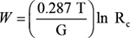


 Eqn.1
Eqn.1


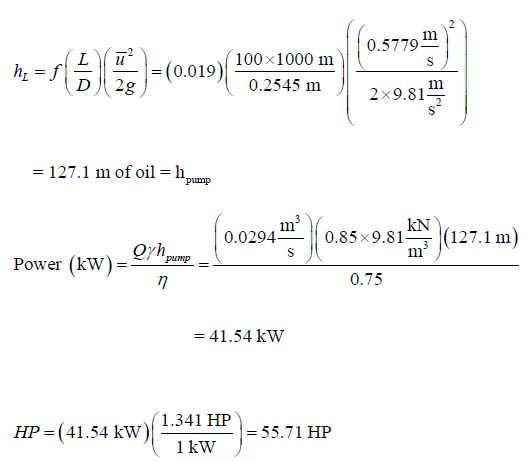


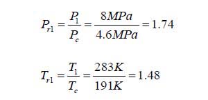


")


")


 & SCADA Systems")


")
")


")
