")
52896WA Advanced Diploma of Civil and Structural Engineering (Materials Testing)
Investigation of the properties of construction materials, the principles which…Read more")
Graduate Diploma of Engineering (Safety, Risk and Reliability)
The Graduate Diploma of Engineering (Safety, Risk and Reliability) program…Read more
Professional Certificate of Competency in Fundamentals of Electric Vehicles
Learn the fundamentals of building an electric vehicle, the components…Read more
Professional Certificate of Competency in 5G Technology and Services Overview
Learn 5G network applications and uses, network overview and new…Read more
Professional Certificate of Competency in Clean Fuel Technology - Ultra Low Sulphur Fuels
Learn the fundamentals of Clean Fuel Technology - Ultra Low…Read more
Professional Certificate of Competency in Battery Energy Storage and Applications
Through a scientific and practical approach, the Battery Energy Storage…Read more
52910WA Graduate Certificate in Hydrogen Engineering and Management
Hydrogen has become a significant player in energy production and…Read more
Professional Certificate of Competency in Hydrogen Powered Vehicles
This course is designed for engineers and professionals who are…Read more
This book will give you a strong understanding of the key underpinning concepts from a very simple understandable point of view.
Revision 5
Website: www.idc-online.com
E-mail: idc@idc-online.com
IDC Technologies Pty Ltd
PO Box 1093, West Perth, Western Australia 6872
Offices in Australia, New Zealand, Singapore, United Kingdom, Ireland, Malaysia, Poland, United States of America, Canada, South Africa and India
Copyright © IDC Technologies 2011. All rights reserved.
First published 2011
All rights to this publication, associated software and workshop are reserved. No part of this publication may be reproduced, stored in a retrieval system or transmitted in any form or by any means electronic, mechanical, photocopying, recording or otherwise without the prior written permission of the publisher. All enquiries should be made to the publisher at the address above.
Disclaimer
Whilst all reasonable care has been taken to ensure that the descriptions, opinions, programs, listings, software and diagrams are accurate and workable, IDC Technologies do not accept any legal responsibility or liability to any person, organization or other entity for any direct loss, consequential loss or damage, however caused, that may be suffered as a result of the use of this publication or the associated workshop and software.
In case of any uncertainty, we recommend that you contact IDC Technologies for clarification or assistance.
Trademarks
All logos and trademarks belong to, and are copyrighted to, their companies respectively.
Acknowledgements
IDC Technologies expresses its sincere thanks to all those engineers and technicians on our training workshops who freely made available their expertise in preparing this manual.
Preface
Have you ever wondered about getting a thorough introduction to the fundamentals of instrumentation, industrial automation and control; thus allowing you to work and perform simple tasks in this key area? In reading this manual and attending the associated course, this could be the opportunity to walk out with a great grounding in the basics of this exciting field which is rapidly changing the way all plants operate. The constant drive to cut costs means that as an operator you will be increasingly having to have more skills and know-how in the plant instrumentation and process control area.
This manual and associated course represents a tremendous opportunity to gain expertise in all the key areas of the fast growing area of industrial automation in two days. Presented by an expert in the area but who is passionate with getting the key chunks of know-how and expertise across to you in a simple understandable manner which you can immediately apply to your job. This is most definitely not a boring lecture style presentation but an intensive learning experience where you will walk away with real skills as a result of the hands-on practical exercises, calculations, case studies and group sessions to ensure an understanding of the concepts and ideas discussed. You will undertake practical sessions at approximately 20 to 30 minute intervals to maximise the absorption rate.
The topics covered commence with an introduction to instrumentation and measurement ranging from pressure, level, temperature and flow devices followed by a review of process control including the all important topic of PID loop tuning. Furthermore, PLC and SCADA systems are covered and the important topics of industrial data communication networks are also examined – again from a very simple understandable point of view. Finally, the manual and course are rounded off with a hands-on review of reading and interpreting simple plant documentation such as P&ID’s so that you can see and understand the operation of the plant through the documentation.
You will gain a strong understanding of the key concepts in instrumentation, process control, SCADA and PLCs.
WHAT YOU WILL LEARN:
- ♦ The fundamentals of instrumentation and process control
- ♦ The basics of PLC’s and SCADA systems
- ♦ An ability to troubleshoot simple problems with instruments, PLC’s and SCADA systems
- ♦ An ability to understand simple plant documentation such as P&ID’s
- ♦ How to work effectively with your instrumentation plant colleagues
PREQUISITES:
The manual and associated course is presented in easy to understand practical language. All you need to benefit from this is a very basic understanding of mathematics and some electrical theory. Contact us for comprehensive pre-course reading and preparation if you are unsure about your level of understanding.
WHO SHOULD READ THIS MANUAL / ATTEND THE COURSE?
Anybody with an interest in gaining know-how in the full range of instrumentation, process control, PLC’s, SCADA and P&ID documentation, this will range from operators, trades personnel, procurement staff, sales staff, technicians and engineers from other backgrounds/disciplines, such as mechanical, electrical and civil. Even the plant secretary who is keen to have a good understanding of the key concepts would benefit. Managers who are keen to understand the key workings and the future of their plants would also benefit from this.
CONTENT SUMMARY
INSTRUMENTATION AND PROCESS CONTROL
INTRODUCTION
- ♦ Overview of instrumentation and control
- ♦ Key building blocks of PLC’s and SCADA systems
- ♦ Outline of the workshop
INTRODUCTION TO PROCESS MEASUREMENT
- ♦ Basic measurement concepts
- ♦ Definition of terminology
- ♦ Measuring instruments and control valves as part of the overall control system
Practical session
PRESSURE MEASUREMENT
- ♦ Principle of pressure measurement
- ♦ Pressure transducers and elements
Practical session
LEVEL MEASUREMENT
- ♦ Principles of level measurement
- ♦ Simple sight glasses
- ♦ Hydrostatic pressure
- ♦ Ultrasonic measurement
- ♦ Electrical measurement
- ♦ Density measurement
Practical session
TEMPERATURE MEASUREMENT
- ♦ Principles of temperature measurement
- ♦ Thermocouples
- ♦ Resistance Temperature Detectors (RTD’s)
- ♦ Thermistors
Practical session
FLOW MEASUREMENT
- ♦ Principles of flow measurement
- ♦ Open channel flow measurement
- ♦ Oscillatory flow measurement
- ♦ Magnetic flow measurement
- ♦ Positive displacement
- ♦ Ultrasonic flow measurement
- ♦ Mass flow measurement
Practical session
FUNDAMENTALS OF PROCESS LOOP TUNING
- ♦ Processes, controllers and tuning
- ♦ PID controllers
- ♦ Gain, dead time and time constants
- ♦ Process noise
- ♦ General purpose closed loop tuning method
Practical session
INTRODUCTION TO CONTROL VALVES
- ♦ Introduction
- ♦ Definition of a control valve
- ♦ Cavitation
- ♦ Flashing
Practical session
DIFFERENT TYPES OF CONTROL VALVES
- ♦ Globe valves
- ♦ Butterfly
- ♦ Eccentric disk
- ♦ Ball
- ♦ Rotary plug
- ♦ Diaphragm and pinch
Practical session
PLC’S, SCADA, AND COMMUNICATIONS
FUNDAMENTALS OF PLCS
- ♦ Introduction to PLC’s
- ♦ Alternative control systems – where do PLC’s fit in?
- ♦ Why PLC’s have become so widely accepted
Practical session
FUNDAMENTALS OF PLC HARDWARE
- ♦ Block diagram of typical PLC
- ♦ PLC processor module – memory organization
- ♦ Input / output section – module types
- ♦ Power supplies
Practical session
FUNDAMENTALS OF PLC SOFTWARE
- ♦ Methods of representing Logic
- ♦ Ladder Logic basics
- ♦ The basic rules for programming
- ♦ Simple PLC programs
Practical session
INTRODUCTION TO SCADA SYSTEMS
- ♦ Fundamentals
- ♦ Comparison of SCADA, DCS, PLC and smart instruments
- ♦ Typical SCADA installations
- ♦ Definition of terms
Practical session
SCADA SYSTEMS HARDWARE
- ♦ Remote Terminal Unit (RTU) structure
- ♦ Analog and digital input/output modules
- ♦ Master site structure
Practical session
SCADA SYSTEMS SOFTWARE
- ♦ Fundamentals
- ♦ Components of a SCADA system
- ♦ Software – design of SCADA packages
- ♦ Configuration of SCADA systems
- ♦ Building the user interface
Practical session
BASICS OF DATA COMMUNICATIONS BETWEEN PLC AND SCADA SYSTEMS
- ♦ Twisted pair cables
- ♦ Fibre optic cables
- ♦ Public network provided services
- ♦ Industrial Ethernet
- ♦ TCP/IP
- ♦ Fieldbus
- ♦ Modbus
- ♦ LAN connectivity: bridges, routers and switches
- ♦ SCADA network security
Practical session
DRAWING TYPES AND STANDARDS
- ♦ Understanding diagram layouts and formats
- ♦ Cross references
- ♦ P&ID’s fundamentals
Practical session
CONCLUSION
- ♦ Summing up and revision of key concepts
- ♦ The future
Contents
1 Introduction 1
1.1 Overview of Instrumentation and control 1
1.2 Key building blocks of PLCs and SCADA systems 2
1.3 Outline of the course 3
2 Introduction to Process Measurement 5
2.1 Basic measurements and control concepts 5
2.2 Definition of terminology 9
2.5 Measuring instruments and control valves as part of the overall control system 11
3 Pressure Measurement 13
3.1 Principles of pressure measurement 13
3.2 Pressure transducers and elements 14
4 Level Measurement 27
4.1 Principles of level measurement 27
4.2 Simple sight glasses 28
4.3 Hydro pressure 29
4.4 Ultrasonic measurement 36
4.5 Electrical measurement 39
4.6 Density measurement 44
5 Temperature Measurement 47
5.1 Principles of temperature measurement 47
5.2 Thermocouples 48
5.3 Resistance Temperature Detectors (RTDs) 49
5.4 Thermistors 52
6 Flow Measurement 53
6.1 Principles of flow measurement 53
6.2 Open channel flow measurement 57
6.3 Oscillatory flow measurement 60
6.4 Magnetic flow meters 67
6.5 Positive displacement 68
6.6 Ultrasonic flow measurement 70
6.7 Mass flow meters 72
7 Fundamentals of Process Loop Tuning 75
7.1 Processes, Controllers and Tuning 75
7.2 Proportional-Integral-Derivative (PID) Controllers 84
7.3 Gain, Dead Time and Time Constants 86
7.4 Process Noise 88
7.5 General Purpose Closed Loop Tuning Method 88
8 Introduction to Control Valves 91
8.1 Introduction 91
8.2 Definition of a Control Valve 92
8.3 Cavitation 99
8.4 Flashing 100
9 Different Types of Control Valves 101
9.1 Introduction 101
9.2 Globe Valves 102
9.3 Butterfly Valves 105
9.4 Eccentric Disk or High Performance Butterfly Valves 106
9.5 Ball Valves 107
9.6 Rotary Plug Valves 110
9.7 Diaphragm Valves 110
9.8 Pinch Valves 111
10 Fundamentals of PLCs 113
10.1 Introduction to the PLC 113
10.2 Alternative Control Systems – where do PLCs fit in? 114
10.3 Why PLCs have become so widely accepted 114
11 Fundamentals of PLC Hardware 119
11.1 Block diagram of typical PLC 119
11.2 PLC processor module – memory organization 120
11.3 Input / Output section – module types 122
11.4 Power Supplies 127
12 Fundamentals of PLC Software 131
12.1 Methods of representing Logic 131
12.2 Ladder Logic Basics 134
12.3 The basic rules for programming 136
13 Introduction to SCADA Systems 139
13.1 Fundamentals 141
13.2 Comparison of SCADA, DCS, PLC and smart instruments 141
13.3 Typical SCADA installations 146
13.4 Definitions of terms 147
14 SCADA Systems Hardware 149
14.1 Remote Terminal Unit (RTU) structure 149
14.2 Analog and digital Input/Output modules 150
14.3 Master site structure 160
15 SCADA System Software 165
15.1 Fundamentals 165
15.2 Components of a SCADA system 166
15.3 Software – design of SCADA packages 168
15.4 Configuration of SCADA systems 173
15.5 Building the user interface 181
16 Basics of Data Communications between PLC and SCADA Systems 189
16.1 Twisted pair cables 189
16.2 Fiber optic cables 192
16.3 Public network provided services 194
16.4 Industrial Ethernet 194
16.5 TCP/IP 197
16.6 Fieldbus 199
16.7 Modbus 201
16.8 LAN Connectivity 208
16.9 SCADA network security 211
17 Drawing Types and Standards 213
17.1 Understanding diagram layouts and formats 213
17.2 Cross references 229
17.3 Piping & Instrumentation Diagrams (P&ID) 229
Appendix A Symbols and Numbering 238
Appendix B Practical Exercises 257
Learning objectives
- Overview of instrumentation and control
- Key building blocks of PLCs and SCADA systems
- Outline of the course
1.1 Overview of instrumentation and control
In an instrumentation and control system, data is acquired by measuring instruments and transmitted to a controller, typically a computer. The controller then transmits data (control signals) to control devices, which act upon a given process.
The integration of systems with each other enables data to be transferred quickly and effectively between different systems in a plant along a data communications link. This eliminates the need for expensive and unwieldy wiring looms and termination points.
Productivity and quality are the principal objectives in the good management of any production activity. Management can be substantially improved by the availability of accurate and timely data. From this, we can surmise that a good instrumentation and control system can facilitate both quality and productivity.
The main purpose of an instrumentation and control system, in an industrial environment, is to provide the following:
- Control of the processes and alarms
- Control of sequencing, interlocking and alarms
- An operator interface for display and control
- Management information
- Distributed Control Systems (DCSs)
- Programmable Logic Controllers (PLCs)
- Supervisory Control and Data Acquisition (SCADA) system
- Smart instrumentation systems
1.2 Key building blocks of PLC and SCADA systems
1.2.1 PLC Systems
In the past, processes were controlled manually, which was a very tedious job. During the early years of control, hard-wired relays were used to control the same process. However, relays could not meet all the needs of modern times, and a faster solution was required. Simply, when a change of control logic was required, the entire hardware wiring needed to be changed. This was time-consuming as well as tiresome. Then, PLCs were developed to automate this process, hence the origin of the so-called “ladder diagram” programming.
Since the late 1970s, PLCs have replaced hard-wired relays with a combination of ladder logic software and solid state electronic input and output modules. They are often used in place of RTUs as they offer a standard hardware solution, which is very economically priced.
The PLCs have become important building blocks for automated systems. Because they have constantly increased in capability while decreasing in cost, PLCs have solidified their position as the device of choice for a wide variety of control tasks.
In brief terms, a PLC is a digital electronic device that contains a programmable (changeable) memory in which a sequence of instructions is stored. Those instructions enable the PLC to perform various useful control functions such as relay logic, counting, timing, sequencing, and arithmetic computation. These functions are usually used to monitor and control individual machines or complex processes via inputs and outputs (I/Os). Input/output modules connected to the PLC provide analogue or digital electronic interfaces to the external world. The PLC reads inputs, processes them through a program, and generates outputs.
1.2.2 SCADA system
A Supervisory Control and Data Acquisition (SCADA) system means a system consisting of a number of Remote Terminal Units (RTUs) collecting field data connected back to a master station via a communications system.
In the first generation of telemetry systems, the objective was to simply have an idea of the system operation. Telemetry is all about remote monitoring. The basic approach was to gather data (generally restricted to measurements of the same type), and relay those results to another location.
These early systems were followed by data acquisition systems, which also captured and stored data. Finally, the control aspect was added as well. It needs to be emphasized that applications of SCADA cover all types of services, not just electrical systems.
SCADA found its first application in the power generation and transmission sectors of the electric utility industry. The interconnection of large power grids in the Midwestern and the Southern U.S. (1962) created the largest synchronized system in the world. The blackout of 1965 prompted the U.S. Federal Power Commission to urge closer coordination between regional coordination groups (Electric Power Reliability Act of 1967), and led to the consequent formation of the National Electric Reliability Council (1970). The importance and urgency of closer coordination was re-emphasized with the northeast blackout of 2003. Transmission SCADA became the base to manage the transmission grid.
In the late 1980s and the early 1990s, when SCADA vendors delivered reasonably priced “small” SCADA systems on low-cost hardware architectures to the small co-ops and municipality utilities, the first real deployments of distribution SCADA systems began. As the market expanded, SCADA vendors who had been providing transmission SCADA began to take notice of the distribution market.
1.3 Outline of the course
The title of the course is – Fundamentals of Instrumentation, Process Control, PLC’s and SCADA for Plant Operators and other Non-Instrument Personnel. This course gives a brief introduction to the measurement and instruments used for measurements. Different types of measurements exist and depending on the type of measurement the instruments used will vary. This will be discussed in detail.
Automation of the control system is gaining prominence due to the ease of controlling facilities it provides. Some of such control systems are PLC, SCADA, DCS and others. These control systems and their components are given in this course. The practical exercises are given which makes the candidate understand the systems in a better way.
Anybody with an interest in gaining know-how in the full range of instrumentation, process control, PLCs, SCADA and P&ID documentation. This can range from operators, trades personnel, procurement staff, sales staff, technicians and engineers from other backgrounds/disciplines, such as mechanical, electrical and civil. Even the plant secretary who is keen to have a good understanding of the key concepts would benefit. Managers who are keen to understand the key workings and the future of their plants would also benefit from this course.
The course mainly covers the following topics:
- Process measurement
- Pressure measurement
- Level measurement
- Temperature measurement
- Flow measurement
- Fundamentals of process loop tuning
- Introduction to control valves
- Different types of control valves
- Fundamentals of PLCs
- Fundamentals of PLC hardware
- Fundamentals of PLC software
- Introduction to SCADA systems
- SCADA systems hardware
- SCADA systems software
- Basics of data communications between PLC and SCADA systems
- Drawing types and standards
In this chapter we will discuss the basic measuring concepts and terminology used. The measurement and control of the overall control system is highlighted.
Learning objectives
- Basic measurement concepts
- Definition of terminology
- Measuring instruments and control valves as part of the overall control system
2.1 Basic measurement concepts
The basic set of units used on this course is the International standard of unit system (SI unit system). This can be summarised in Table 2.1.
| Quantity | Unit | Abbreviation |
|---|---|---|
| Length | Meter | m |
| Mass | Kilogram | kg |
| Time | Second | s |
| Current | Ampere | A |
| Temperature | Degrees kelvin | °K |
| Voltage | Volt | V |
| Resistance | Ohm | Ω |
| Capacitance | Farad | F |
| Inductance | Henry | H |
| Energy | Joules | J |
| Power | Watt | W |
| Frequency | Hertz | Hz |
| Charge | Coulomb | C |
| Force | Newton | N |
| Magnetic flux | Weber | Wb |
| Magnetic field | Webers/metre2 | Wb/m2 |
| Density | Kilogram/metre3 | kg/m3 |
There are a number of criteria that must be satisfied when specifying process measurement equipment. Below is a list of the more important specifications.
2.1.1 Accuracy
The accuracy specified by a device is the amount of error that may occur when measurements are taken. It determines how precise or correct the measurements are to the actual value and is used to determine the suitability of the measuring equipment. Accuracy can be expressed as any of the following:
- Error in units of the measured value
- Percent of span
- Percent of upper range value
- Percent of scale length
- Percent of actual output value
Accuracy generally contains the total error in the measurement and accounts for linearity, hysteresis and repeatability. Figure 2.1 shows errors in measurement.
Reference accuracy is determined at reference conditions, i.e. constant ambient temperature, static pressure, and supply voltage. There is also no allowance for drift over time.
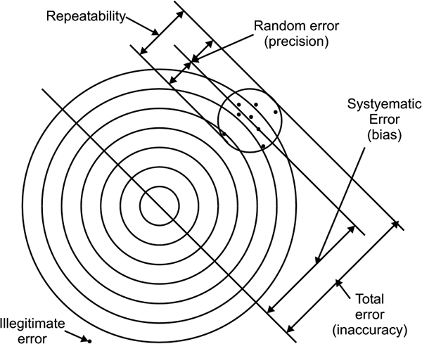
Accuracy terminology
2.1.2 Range of operation
The range of operation defines the high and low operating limits between which the device will operate correctly, and at which the other specifications are guaranteed. Operation outside of this range can result in excessive errors, equipment malfunction and even permanent damage or failure.
2.1.3 Budget/Cost
Although not so much a specification, the cost of the equipment is certainly a selection consideration. This is generally dictated by the budget allocated for the application. Even if all the other specifications are met, this can prove an inhibiting factor.
2.1.4 Hysteresis
Hysteresis is the difference in the output for given input when the input is increasing and output for same input when input is decreasing. In other words, it is the difference in the way device works when moving from 0% to 100%, compared to the way the device works when moving from 100% to 0%. When input of any instrument is slowly varied from zero to full scale and then back to zero, its output varies. One example is shown in Figure 2.2. This is where the accuracy of the device is dependent on the previous value and the direction of variation. Hysteresis causes a device to show an inaccuracy from the correct value, as it is affected by the previous measurement.

Hysteresis
2.1.5 Linearity
Linearity expresses the deviation of the actual reading from a straight line. If all outputs are in the same proportion to corresponding inputs over a span of values, then input-output plot is straight line else it will be non linear as shown in Figure 2.3. For continuous control applications, the problems arise due to the changes in the rate the output differs from the instrument. The gain of a non-linear device changes as the change in output over input varies. In a closed loop system, changes in gain affect the loop dynamics. In such an application, the linearity needs to be assessed. If a problem does exist, then the signal needs to be linearised.
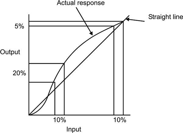
Linearity
2.1.6 Repeatability
Repeatability defines how close a second measurement is to the first under the same operating conditions, and for the same input. Repeatability is generally within the accuracy range of a device and is different from hysteresis in that the operating direction and conditions must be the same.
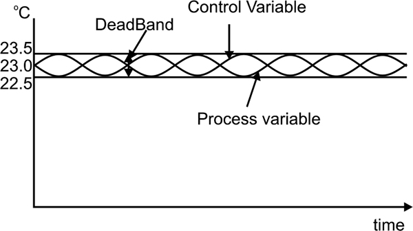
Continuous control applications can be affected by variations due to repeatability. When a control system sees a change in the parameter it is controlling, it will adjust its output accordingly. However if the change is due to the repeatability of the measuring device, then the controller will over-control. This problem can be overcome by using the deadband in the controller as shown in Figure 1.4; however repeatability becomes a problem when an accuracy of say, 0.1% is required, and a repeatability of 0.5% is present.
Repeatability
Ripples or small oscillations can occur due to over controlling. This needs to be accounted for in the initial specification of allowable values.
2.1.7 Response
When the output of a device is expressed as a function of time (due to an applied input) the time taken to respond can provide critical information about the suitability of the device. A slow responding device may not be suitable for an application. This typically applies to continuous control applications where the response of the device becomes a dynamic response characteristic of the overall control loop. However in critical alarming applications where devices are used for point measurement, the response may be just as important. Figure 1.5 shows response of the system to a step input.
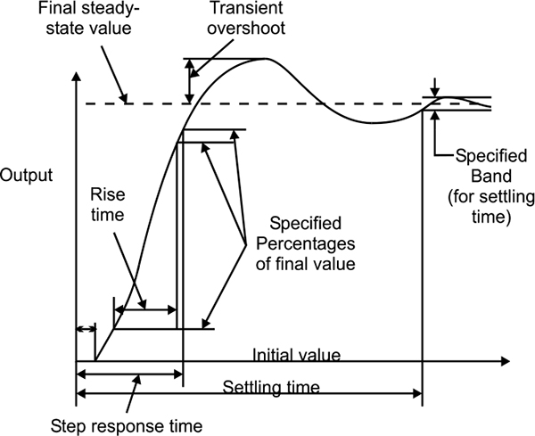
Typical time response for a system with a step input
2.2 Definition of terminology
Accuracy: How precise or correct the measured value is to the actual value. Accuracy is an indication of error in the measurement.
Ambient: The surrounds or environment in reference to a particular point or object.
Attenuation: A decrease in signal magnitude over a period of time.
Calibrate: To configure a device so that the required output represents (to a defined degree of accuracy) the respective input.
Closed loop: Relates to a control loop where the process variable is used to calculate the controller output.
Coefficient, temperature: A coefficient is typically a multiplying factor. The temperature coefficient defines how much change in temperature there is for a given change in resistance (for a temperature dependent resistor).
Cold junction: The thermocouple junction which is at a known reference temperature.
Compensation: A supplementary device used to correct errors due to variations in operating conditions.
Controller: A device which operates automatically to regulate the control of a process with a control variable.
Elastic: The ability of an object to regain its original shape when an applied force is removed. When a force is applied that exceeds the elastic limit, then permanent deformation will occur.
Excitation: The energy supply required to power a device for its intended operation.
Gain: This is the ratio of the change of the output to the change in the applied input. Gain is a special case of sensitivity, where the units for the input and output are identical and the gain is unit less.
Hunting: Generally an undesirable oscillation at or near the required set point. Hunting typically occurs when the demands on the system performance are high and possibly exceed the system capabilities. The output of the controller can be over controlled due to the resolution of accuracy limitations.
Hysteresis: The accuracy of the device is dependent on the previous value and the direction of variation. Hysteresis causes a device to show an inaccuracy from the correct value, as it is affected by the previous measurement.
Ramp: Defines the delayed and accumulated response of the output for a sudden change in the input.
Range: The region between the specified upper and lower limits where a value or device is defined and operated.
Reliability: The probability that a device will perform within its specifications for the number of operations or time period specified.
Repeatability: The closeness of repeated samples under exact operating conditions.
Reproducibility: The similarity of one measurement to another over time, where the operating conditions have varied within the time span, but the input is restored.
Resolution: The smallest interval that can be identified as a measurement varies.
Resonance: The frequency of oscillation that is maintained due to the natural dynamics of the system.
Response: Defines the behaviour over time of the output as a function of the input. The output is the response or effect, with the input usually noted as the cause.
Self Heating: The internal heating caused within a device due to the electrical excitation. Self heating is primarily due to the current draw and not the voltage applied, and is typically shown by the voltage drop as a result of power (I2R) losses.
Sensitivity: This defines how much the output changes, for a specified change in the input to the device.
Set-point: Used in closed loop control, the set point is the ideal process variable. It is represented in the units of the process variable and is used by the controller to determine the output to the process.
Span Adjustment: The difference between the maximum and minimum range values. When provided in an instrument, this changes the slope of the input-output curve.
Steady state: Used in closed loop control where the process no longer oscillates or changes and settles at some defined value.
Stiction: Shortened form of static friction, and defined as resistance to motion. More important is the force required (electrical or mechanical) to overcome such a resistance.
Stiffness: This is a measure of the force required to cause a deflection of an elastic object.
Thermal shock: An abrupt temperature change applied to an object or device.
Time constant: Typically a unit of measure which defines the response of a device or system. The time constant of a first order system is defined as the time taken for the output to reach 63.2% of the total change, when subjected to a step input change.
Transducer: An element or device that converts information from one form (usually physical, such as temperature or pressure) and to another (usually electrical, such as volts or milli volts or resistance change). A transducer can be considered to comprise a sensor at the front end (at the process) and a transmitter.
Transient: A sudden change in a variable which is neither a controlled response nor long lasting.
Transmitter: A device that converts from one form of energy to another. Usually from electrical to electrical for the purpose of signal integrity for transmission over longer distances and for suitability with control equipment.
Variable: Generally, this is some quantity of the system or process. The two main types of variables that exist in the system are the measured variable and the controlled variable. The measured variable is the measured quantity and is also referred to as the process variable as it measures process information. The controlled variable is the controller output which controls the process.
Vibration: This is the periodic motion (mechanical) or oscillation of an object.
Zero adjustment: The zero in an instrument is the output provided when no or zero input is applied. The zero adjustment produces a parallel shift in the input-output curve.
2.3 Measuring instruments and control valves as part of the overall control system
Figure 2.6 shows how instrument and control valves fit into the overall control system structure. The topic of controllers and tuning forms part of a separate workshop.

Instruments and control valves in the overall control system
2.3.1 Typical applications
Some typical applications are listed below:
HVAC (Heating, ventilation and air conditioning) applications
- Heat transfer
- Billing
- Axial fans
- Climate control
- Hot and chilled water flows
- Forced air
- Fumehoods
- System balancing
- Pump operation and efficiency
Petrochemical applications
- Co-generation
- Light oils
- Petroleum products
- Steam
- Hydrocarbon vapours
- Flare lines, stacks
Natural gas
- Gas leak detection
- Compressor efficiency
- Fuel gas systems
- Bi-directional flows
- Mainline measurement
- Distribution lines measurement
- Jacket water systems
- Station yard piping
Power industry
- Feed water
- Circulating water
- High pressure heaters
- Fuel oil
- Stacks
- Auxiliary steam lines
- Cooling tower measurement
- Low pressure heaters
- Reheat lines
- Combustion air
Emissions monitoring
- Chemical incinerators
- Trash incinerators
- Refineries
- Stacks and rectangular ducts
- Flare lines
In this chapter we will discuss the principles of pressure measurement and pressure transducers. Both mechanical and electrical elements are highlighted.
Learning objectives
- Principle of pressure measurement
- Pressure transducers and elements
3.1 Principle of pressure measurement
3.1.1 Bar and Pascal
Pressure is defined as a force per unit area, and can be measured in units such as psi (pounds per square inch), inches of water, and milli-meters of mercury, Pascal (Pa, or N/m�) or bar. Until the introduction of SI units, the ‘bar’ was quite common.
The bar is equivalent to 100,000 N/m�, which were the SI units for measurement. To simplify the units, the N/m� was adopted with the name of Pascal, abbreviated to Pa. Pressure is quite commonly measured in kilopascals (kPa), which is 1000 Pascal and equivalent to 0.145psi.
3.1.2 Absolute, gauge and differential pressure
The Pascal is a means of measuring a quantity of pressure. When the pressure is measured in reference to an absolute vacuum (no atmospheric conditions), then the result will be in Pascal (Absolute). However when the pressure is measured relative to the atmospheric pressure, then the result will be termed Pascal (Gauge). If the gauge is used to measure the difference between two pressures, it then becomes Pascal (Differential).
Note 1: It is common practice to show gauge pressure without specifying the type, and to specify absolute or differential by stating ‘absolute’ or ‘differential’ for those pressures.
Note 2: Older measurement equipment may be in terms of psi (pounds per square inch) and as such represent gauge and absolute pressure as psig and psia respectively. Note that the ‘g’ and ‘a’ are not recognized in the SI unit symbols, and as such are no longer encouraged.
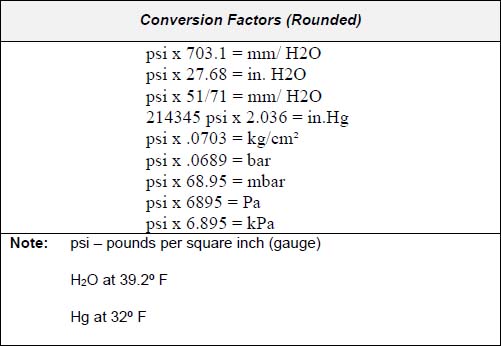
To determine differential in inches of mercury vacuum multiply psi by 2.036 (or approximately 2). Another common conversion is 1 Bar = 14.7 psi. Table 3.1 shows different conversion factors.
Conversion Factor
3.2 Pressure transducers and elements
In this section we have discussed about pressure transducers and elements in mechanical and electrical.
3.2.1 Pressure transducers and elements – mechanical
Mechanical pressure transducers and elements are as follows
- Bourdon tube
- Helix and spiral tubes
- Spring and bellows
- Diaphragm
- Manometer
- Single and Double inverted bell
Bourdon Tube
The Bourdon tube works on a simple principle that a bent tube will change its shape when exposed to variations of internal and external pressure. As pressure is applied internally, the tube straightens and returns to its original form when the pressure is released.
The tip of the tube moves with the internal pressure change and is easily converted with a pointer onto a scale. A connector link is used to transfer the tip movement to the geared movement sector. The pointer is rotated through a toothed pinion by the geared sector.
This type of gauge may require vertical mounting (orientation dependent) for correct results. The element is subject to shock and vibration, which is also due to the mass of the tube. Because of this and the amount of movement with this type of sensing, they are prone to breakage, particularly at the base of the tube.
The main advantage with the Bourdon tube is that it has a wide operating range (depending on the tube material). This type of pressure measurement can be used for positive or negative pressure ranges, although the accuracy is impaired when in a vacuum.
Selection and Sizing: The type of duty is one of the main selection criteria when choosing Bourdon tubes for pressure measurement. For applications, which have rapid cycling of the process pressure, such in ON/OFF controlled systems, then the measuring transducer requires an internal snubber. They are also prone to failure in these applications.
Liquid filled devices are one way to reduce the wear and tear on the tube element.
Advantages
- Inexpensive
- Wide operating range
- Fast response
- Good sensitivity
- Direct pressure measurement
Disadvantages
- Primarily intended for indication only
- Non-linear transducer, linearised by gear mechanism
- Hysteresis on cycling
- Sensitive to temperature variations
- Limited life when subject to shock and vibration
Application Limitations: These devices should be used in air if calibrated for air, and in liquid if calibrated for liquid. Special care is required for liquid applications in bleeding air from the liquid lines.
Figure 3.1 shows pressure measurement using C type Bourdon Tube. This type of pressure measurement is limited in applications where there is input shock (a sudden surge of pressure), and in fast moving processes.
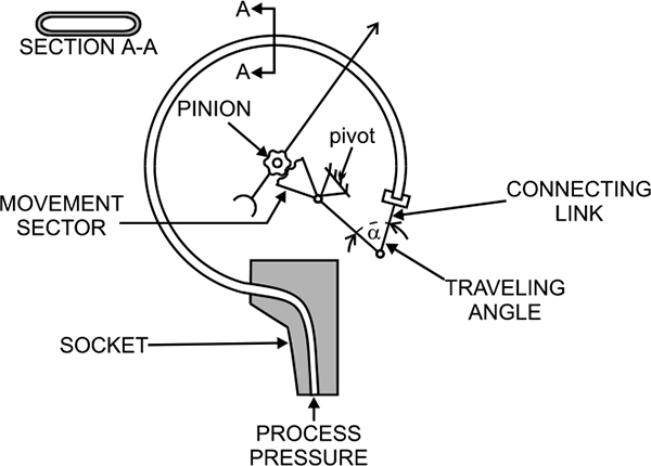
C-Bourdon pressure element
If the application is for the use of oxygen, then the device cannot be calibrated using oil. Lower ranges are usually calibrated in air. Higher ranges, usually 1000kPa, are calibrated with a dead weight tester (hydraulic oil).
Helix and spiral tubes
Helix and spiral tubes are fabricated from tubing into shapes as per their naming. With one end sealed, the pressure exerted on the tube causes the tube to straighten out. The amount of straightening or uncoiling is determined by the pressure applied.
These two approaches use the Bourdon principle. The uncoiling part of the tube is mechanically linked to a pointer which indicates the applied pressure on a scale. This has the added advantage over the Bourdon tube, as there are no movement losses due to links and levers.
The Spiral tube is suitable for pressure ranges up to 28,000 kPa and the helical tube for ranges up to 500,000 kPa. The pressure sensing elements vary depending on the range of operating pressure and type of process involved.
The choice of spiral or helical elements is based on the pressure ranges. The pressure level between spiral and helical tubes varies depending on the manufacturer. Low pressure elements have only two or three coils to sense the span of pressures required, however high pressure sensing may require up to 20 coils. Figure 3.2 shows pressure measurement using spiral bourdon element.
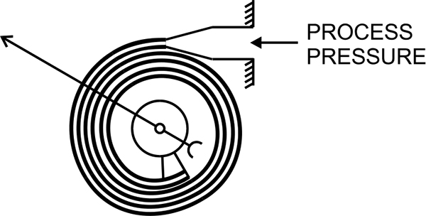
Spiral bourdon element
One difference and advantage of these is the dampening they have with fluids under pressure.
The advantages and disadvantages of this type of measurement are similar to the Bourdon tube with the following differences
Advantages
- Increased accuracy and sensitivity
- Higher over range protection
Disadvantages
- Very expensive
Application Limitations: Process pressure changes cause problems with the increase in the coil size.
Spring and bellows
A bellows is an expandable element and is made up of a series of folds, which allow expansion. One end of the Bellows is fixed and the other moves in response to the applied pressure. A spring is used to oppose the applied force and a linkage connects the end of the bellows to a pointer for indication. Bellows type sensors are also available which have the sensing pressure on the outside and the atmospheric conditions within.
The spring is added to the bellows for more accurate measurement. The elastic action of the bellows by themselves is insufficient to precisely measure the force of the applied pressure.
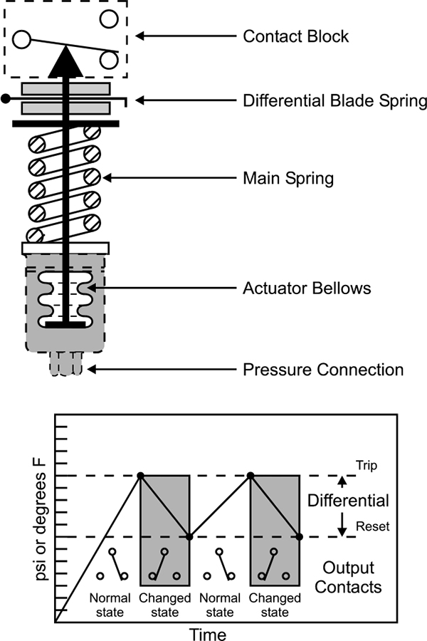
This type of pressure measurement is primarily used for ON/OFF control providing clean contacts for opening and closing electrical circuits. This form of sensing responds to changes in pneumatic or hydraulic pressure. Figure 3.3 shows pressure measurement using bellows.
Typical Application: The process pressure is connected to the sensor and is applied directly into the bellows. As the pressure increases, the bellows exert force on the main spring. When the threshold force of the main spring is overcome, the motion is transferred to the contact block causing the contacts to actuate. This is the Trip setting.
When the pressure decreases, the main spring will retract which causes the secondary differential blade spring to activate and reset the contacts. This is the Reset setting.
The force on the main spring is varied by turning the operating range adjustment screw. This determines where the contacts will trip.
The force on the secondary differential blade spring is varied by turning the differential adjustment screw. This determines where the contacts will reset. Figure 3.4 shows working of bellows graphically.
Basic mechanical structure
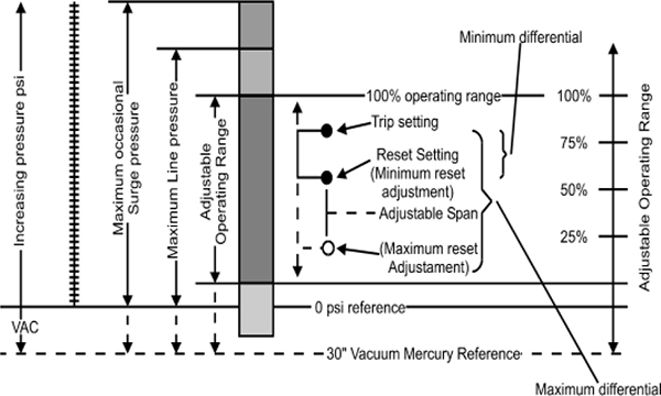
Graphical illustration of technical terms
Copper alloy bellows may be used on water or air. Other liquids and gases may be used if non-corrosive to this alloy. Use type 316 stainless steel for more corrosive liquids or gases.
Diaphragm
Many pressure sensors depend on the deflection of a diaphragm for measurement. The diaphragm is a flexible disc, which can be either flat or with concentric corrugations and is made from sheet metal with high tolerance dimensions.
The diaphragm can be used as a means of isolating the process fluids, or for high-pressure applications. It is also useful in providing pressure measurement with electrical transducers.
Diaphragms are well developed and proven. Modern designs have negligible hysteresis, friction and calibration problems when used with smart instrumentation. They are used extensively on air conditioning plants and for ON/OFF switching applications.
Selection: The selection of diaphragm materials is important, and is very much dependent on the application. Beryllium copper has good elastic qualities, where Ni-Span C has a very low temperature coefficient of elasticity.
Stainless steel and Inconel are used in extreme temperature applications, and are also suited for corrosive environments. For minimum hysteresis and drift, then Quartz is the best choice. There are two main types of construction and operation of diaphragm sensors. They are
- Motion Balanced
- Force Balanced
Motion balanced designs are used to control local, direct reading indicators. They are however more prone to hysteresis and friction errors.
Force balanced designs are used as transmitters for relaying information with a high accuracy; however they do not have direct indication capability.
Advantages
- Provide isolation from process fluid
- Good for low pressure
- Inexpensive
- Wide range
- Reliable and proven
- Used to measure gauge, atmospheric and differential pressure
Manometer
The simplest form of a manometer is that of a U-shaped tube filled with liquid. The reference pressure and the pressure to be measured are applied to the open ends of the tube. If there is a difference in pressure, then the heights of the liquid on the two sides of the tube will be different.
This difference in the heights is the process pressure in mm of water (or mm of mercury). The conversion into kPa is quite simple
For water, Pa = mm H2O x 9.807
For mercury, Pa = mm Hg x 133.3
Typical Applications: This type of pressure measurement is mainly used for spot checks or for calibration. They are used for low range measurements, as higher measurements require mercury. Mercury is toxic and is therefore considered mildly hazardous. Figure 3.5 shows simplest form of manometer for pressure measurement.
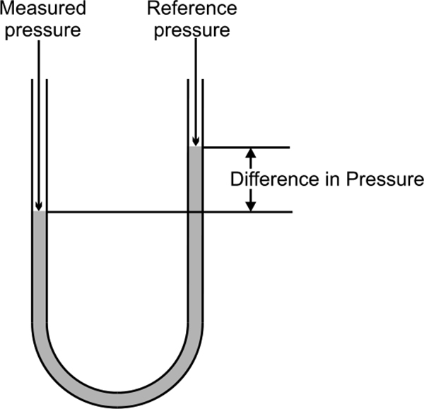
Simplest form of manometer
Advantages
- Simple operation and construction
- Inexpensive
Disadvantages
- Low-pressure range (water)
- Higher-pressure range requires mercury
- Readings are localised
Application Limitations: Manometers are limited to a low range of operation due to size restrictions. They are also difficult to integrate into a continuous control system.
Single and double inverted bell
The Bell instrument measures the pressure difference in a compartment on each side of a bell-shaped chamber. If the pressure to be measured is referenced to the surrounding conditions, then the lower compartment is vented to the atmosphere and gauge pressure is measured. If the lower compartment is evacuated to form a vacuum, then the pressure measured will be in absolute units. However, to measure differential pressure, the higher pressure is connected to the top of the chamber and the lower pressure to the bottom. Figure 3.6 shows bell instrument for pressure measurement.
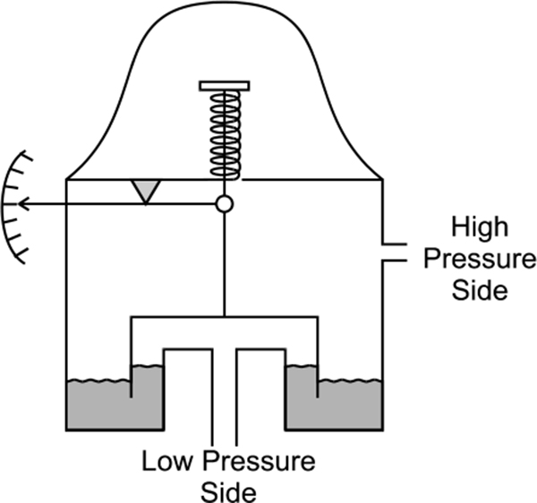
Inverted bell d/p detector
The bell instrument is used in applications where very low pressures are required to be measured, typically in the order of 0-250 Pa.
3.2.2 Pressure transducers and elements – electrical
The typical range of transducers here are:
- Strain gauge
- Vibrating wire
- Piezoelectric
- Capacitance
- Linear Variable Differential Transformer
- Optical
Strain gauge
Strain gauge sensing uses a metal wire or semiconductor chip to measure changes in pressure. A change in pressure causes a change in resistance as the metal is deformed. This deformation is not permanent, as the pressure (applied force) does not exceed the elastic limit of the metal. If the elastic limit is exceeded than permanent deformation will occur.
This is commonly used in a Wheatstone bridge arrangement where the change in pressure is detected as a change in the measured voltage.
Strain gauges in their infancy were metal wires supported by a frame. Advances in the technology of bonding materials mean that the wire can be adhered directly to the strained surface. Since the measurement of strain involves the deformation of metal, the strain material need not be limited to being a wire. As such, further developments also involve metal foil gauges. Bonded strain gauges are the more commonly used type. Figure 3.7 shows simple Wheatstone circuit for strain gauge.
As strain gauges are temperature sensitive, temperature compensation is required. One of the most common forms of temperature compensation is to use a wheatstone bridge. Apart from the sensing gauge, a dummy gauge is used which is not subjected to the forces but is also affected by temperature variations. In the bridge arrangement the dummy gauge cancels with the sensing gauge and eliminates temperature variations in the measurement.
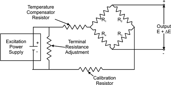
Wheatstone circuit for strain gauges32
Strain gauges are mainly used due to their small size and fast response to load changes.
Typical Application: Pressure is applied to an isolating diaphragm, where the force is transmitted to the poly-silicon sensor by means of a silicone fill fluid. The reference side of the sensor is exposed to atmospheric pressure for gauge pressure transmitters. A sealed vacuum reference is used for absolute pressure transmitters.
When the process pressure is applied to the sensor, this creates a small deflection of the sensing diaphragm, which applies strain to the Wheatstone bridge circuit within the sensor. The change in resistance is sensed and converted to a digital signal for processing by the microprocessor.
Selection and Sizing: There exists a very wide selection of strain gauge transducers, in range, accuracy and the associated cost.
Advantages
- Wide range, 7.5kPa to 1400 MPa
- Inaccuracy of 0.1%
- Small in size
- Stable devices with fast response
- Most have no moving parts
- Good over-range capability
Disadvantages
- Unstable due to bonding material
- Temperature sensitive
- Thermo elastic strain causes hysteresis
Application Limitations: All strain gauge applications require regulated power supplies for the excitation voltage, although this is commonly internal with the sensing circuits.
Vibrating wire
This type of sensor consists of an electronic oscillator circuit, which causes a wire to vibrate at its natural frequency when under tension. The principle is similar to that of a guitar string. The vibrating wire is located in a diaphragm. As the pressure changes on the diaphragm so does the tension on the wire, which affects the frequency that the wire vibrates or resonates at. These frequency changes are a direct consequence of pressure changes and as such are detected and shown as pressure.
The frequency can be sensed as digital pulses from an electromagnetic pickup or sensing coil. An electronic transmitter would then convert this into an electrical signal suitable for transmission.
This type of pressure measurement can be used for differential, absolute or gauge installations. Absolute pressure measurement is achieved by evacuating the low-pressure diaphragm. A typical vacuum pressure for such a case would be about 0.5 Pa.
Advantages
- Good accuracy and repeatability
- Stable
- Low hysteresis
- High resolution
- Absolute, gauge or differential measurement
Disadvantages
- Temperature sensitive
- Affected by shock and vibration
- Non-linear
- Physically large
Application Limitations: Temperature variations require temperature compensation within the sensor this problem limits the sensitivity of the device. The output generated is non-linear which can cause continuous control problems.
This technology is seldom used any more. Being older technology it is typically found with analogue control circuitry.
Piezoelectric
When pressure is applied to crystals, they are elastically deformed. Piezoelectric pressure sensing involves the measurement of such deformation. When a crystal is deformed, an electric charge is generated for only a few seconds. The electrical signal is proportional to the applied force.
Because these sensors can only measure for a short period, they are not suitable for static pressure measurement. More suitable measurements are made of dynamic pressures caused from:
- Shock
- Vibration
- Explosions
- Pulsations
- Engines
- Compressors
This type of pressure sensing does not measure static pressure, and as such requires some means of identifying the pressure measured. As it measures dynamic pressure, the measurement needs to be referenced to the initial conditions before the impact of the pressure disturbance. The pressure can be expressed in relative pressure units, Pascal relative.
Quartz is commonly used as the sensing crystal as it is inexpensive, stable and insensitive to temperature variations. Tourmaline is an alternative, which gives faster response speeds, typically in the order of microseconds.
Advantages
- Accuracy 0.075%
- Very high pressure measurement, up to 70MPa
- Small size
- Robust
- Fast response, < 1 nanosecond
- Self-generated signal
Disadvantages
- Dynamic sensing only
- Temperature sensitive
Application Limitations: Require special cabling and signal conditioning.
Capacitance
Capacitive pressure measurement involves sensing the change in capacitance that results from the movement of a diaphragm. The sensor is energised electrically with a high frequency oscillator. Figure 3.8 shows cross section of Rosemount sensor. When the diaphragm is deflected due to pressure changes, the relative capacitance is measured by a bridge circuit. Figure 3.9 shows capacitance pressure detector.
Two designs are quite common. The first is the two-plate design and is configured to operate in the balanced or unbalanced mode. The other is a single capacitor design.
The balanced mode is where the reference capacitor is varied to give zero voltage on the output. The unbalanced mode requires measuring the ratio of output to excitation voltage to determine pressure. This type of pressure measurement is quite accurate and has a wide operating range. Capacitive pressure measurement is also quite common for determining the level in a tank or vessel.
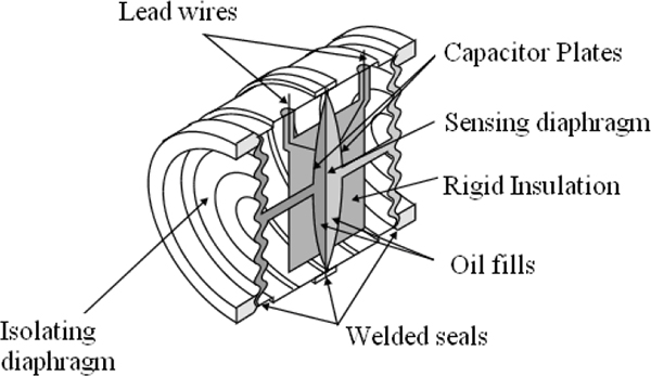
Cross section of the Rosemount S-Cell™ Sensor (Courtesy of Rosemount)
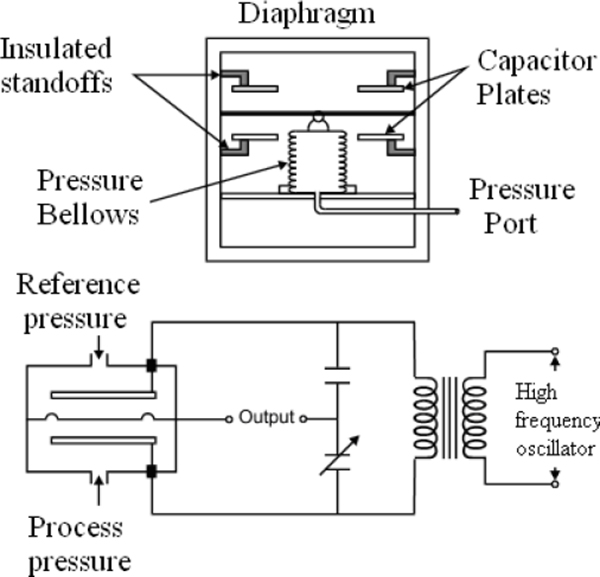
Capacitance pressure detector
Advantages
- Inaccuracy 0.01 to 0.2%
- Range of 80Pa to 35MPa
- Linearity
- Fast response
Disadvantages
- Temperature sensitive
- Stray capacitance problems
- Vibration
- Limited overpressure capability
- Cost
Application Limitations: Many of the disadvantages above have been addressed and their problems reduced in newer designs. Temperature controlled sensors are available for applications requiring a high accuracy.
With strain gauges being the most popular form of pressure measurement, capacitance sensors are the next most common solution.
Linear Variable Differential Transformers (LVDT)
This type of pressure measurement relies on the movement of a high permeability core within transformer coils. The movement is transferred from the process medium to the core by use of a diaphragm, bellows or bourdon tube.
The LVDT operates on the inductance ratio between the coils. Three coils are wound onto the same insulating tube containing the high permeability iron core. The primary coil is located between the two secondary coils and is energised with an alternating current.
Equal voltages are induced in the secondary coils if the core is in the centre. The voltages are induced by the magnetic flux. When the core is moved from the centre position, the result of the voltages in the secondary windings will be different. The secondary coils are usually wired in series. Figure 3.10 shows LVDT for measurement of pressure.
LVDTs are sensitive to vibration and are subject to mechanical wear.
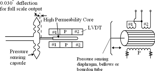
Linear variable differential transformer
Disadvantages
- Mechanical wear
- Vibration
Optical
Optical sensors can be used to measure the movement of a diaphragm due to pressure. An opaque vane is mounted to the diaphragm and moves in front of an infrared light beam. As the light is disturbed, the received light on the measuring diode indicates the position of the diaphragm.
A reference diode is used to compensate for the ageing of the light source. Also, by using a reference diode, the temperature effects are nullified as they affect the sensing and reference diodes in the same way.
Advantages
- Temperature corrected
- Good repeatability
- Negligible hysteresis
Disadvantages
- Expensive
Learning objectives
- Principles of level measurement
- Simple sight glasses
- Hydrostatic pressure
- Ultrasonic measurement
- Electrical measurement
- Density measurement
4.1 Principle of level measurement
4.1.1 Continuous measurement
The units of level are metres (m). However, there are numerous ways to measure level that require different technologies and various units of measurement.
Such means may be
- Ultrasonic, transit time
- Pulse echo
- Pulse radar
- Pressure, hydrostatic
- Weight, strain gauge
- Conductivity
- Capacitive
For continuous measurement, the level is detected and converted into a signal that is proportional to the level. Microprocessor based devices can indicate level or volume.
Different techniques also have different requirements. For example, when detecting the level from the top of a tank, the shape of the tank is required to deduce volume.
When using hydrostatic means, which detects the pressure from the bottom of the tank, the density must be known and remain constant.
4.1.2 Point detection
Point detection can also be provided for all liquids and solids. Some of the more common types are:
- Capacitive
- Microwave
- Radioactive
- Vibration
- Conductive
A level measuring system often consists of the sensor and a separate signal conditioning instrument. This combination is often chosen when multiple outputs (continuous and switched) are required and parameters may need to be altered.
4.2 Simple sight glasses
A visual indication of the level can be obtained when part of the vessel is constructed from transparent material or the liquid in a vessel is bypassed through a transparent tube. The advantage of using stop valves with the use of a bypass pipe is the ease in removal for cleaning. Figure 4.1 shows level measurement using visual inspection.
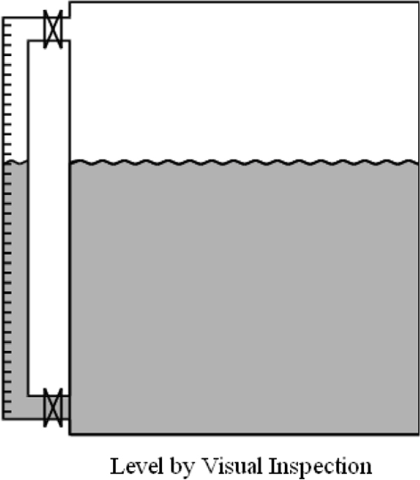
Level by Visual Inspection
Advantages
- Very simple
- Inexpensive
Disadvantages
- Not suitable for automated control
- Maintenance – requires cleaning
- Fragile – easily damaged
Applications/Limitations
These are not highly suited for industrial applications as manual viewing and transfer of information is required by the operator.
Applications of such level measuring devices can be seen in tanks for the storage of lubricating oils or water. They provide a very simple means of accessing level information and can simplify the task of physically viewing or dipping a tank. They are, however, generally limited to operator inspection.
Sight glasses are also not suitable for dark or dirty liquids. This type should not be used when measuring hazardous liquids as the glass-tube is easily damaged or broken. In installations where the gauge is at a lower temperature than the process condensation can occur outside the gauge, impairing the accuracy of the reading.
4.3 Hydro pressure
Some of the different types of level measurement with pressure are:
- Static pressure
- Differential pressure
- Bubble tube method
- Diaphragm Box
- Weighing
4.3.1 Static pressure
The basis of hydrostatic pressure measurement for level is such that the measured pressure is proportional to the height of liquid in the tank, irrespective of volume. The pressure is related to the height by the following:
Where: P = pressure
h = height
ρ = relative density of fluid
g = acceleration due to gravity

For constant density, the only variable that changes is the height. In fact, any instrument that can measure pressure can be calibrated to read height of a given liquid, and can be used to measure liquid level in vessels under atmospheric conditions.
Most pressure sensors compensate for atmospheric conditions, so the pressure on the surface of liquids open to the atmosphere will be zero. The measuring units are generally in Pascal, but note that 10 Pa is approximately equivalent to 1 mm head of water.
Easy to remember ? 100 kPa = 10 m head of water = 1 bar = 1 atm
Actual numbers ? 101.325 kPa = 10.333 m head of water = 1.01325 bar = 1 atm
Hydrostatic pressure transducers always consist of a membrane, which is connected either mechanically or hydraulically to a transducer element. The transducer element can be based on such technologies as inductance, capacitance, strain gauge or even semiconductor. Figure 4.2 shows level measurement using pressure gauge.
A pressure gauge used to measure the height of a liquid in an open tank
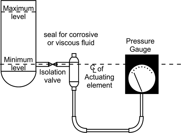
The pressure transducer can be mounted in many types of pressure sensor so that the application can be quite specific to the requirement of the process conditions. Since the movement of the membrane is only a few microns, the semiconductor transducer is extremely insensitive to dirt or product build-up. This makes this type of measurement useful for such applications as sewage water, sludge, paint and oils. A seal is required for corrosive or viscous liquids or in the case where a pipe is used to hydraulically transmit the pressure to a gauge.
Since there is no application of movement, there is no relaxing force to cause hysteresis.
A pressure sensor is exposed to the pressure of the system, and therefore needs to be mounted at or near the bottom of the vessel. In situations where it is not possible to mount the sensor directly in the side of the vessel at the appropriate depth, it can be mounted from the top of the vessel and lowered into the fluid on the end of a rod or cable. This method is commonly used for applications in reservoirs and deep wells.
If the use of extension nozzles or long pipes is unavoidable, precautions are required to ensure the fluid will not harden or congeal in the pipe. If this occurs, then the pressure detected will no longer be accurate. Different mounting systems or pipe heaters could be used to prevent this.
Static pressure is measured in this type of measurement. The sensor therefore, should not be mounted directly in the product stream as the pressure measured will be too high and the level reading inaccurate. For similar reasons, a pressure sensor should not be mounted in the discharge outlet of a vessel, as the pressure measurement will be incorrectly low during discharge.
Advantages
- Level or volume measurement
- Simple to assemble and install
- Simple to adjust
- Reasonably accurate
Disadvantages
- Dependent on relative density of material
- More expensive than simpler types
- Expensive for high accuracy applications
Application Limitations
Level measurement can be made using the hydrostatic principle in open tanks, when the density of the material is constant. The sensor needs to be mounted in an open tank to ensure that the liquid, even at the minimum level always covers the process diaphragm.
Since the sensor is measuring pressure, it is therefore sensitive to sludge and dirt on the bottom of the tank. Build-up can often occur around or in the flange where the sensor is mounted. Bore water can also cause calcium build-up.
It is also critical that the pressure measurement is referenced to atmospheric conditions.
Level Measurement with Changing Product Density
If the material being measured is of varying densities, then accurate level measurement is impaired. However, sensors are available that compensate for various densities. In such sensors, mounting an external limit switch at a known height above the sensor makes corrections. When the switch status changes, the sensor uses the current measured value to automatically compensate for any density change.
It is optimal to mount the external limit switch for this compensation at the point where the level increases or decreases. This correction for density changes is best when the distance between the limit switch and the sensor is made as large as possible.
Variations in the temperature also affect the density of the fluid. Wax is a big problem where the pipes are heated with even slight variations in temperature cause noticeable changes in the density.
Volume Measurement for Different Vessel Shapes
Level measurement is easily obtained by hydrostatic pressure; however the volume of fluid within a vessel relies on the shape of the vessel. If the shape of the vessel does not change for increasing height then the volume is simply the level multiplied by the cross-sectional area. But, if the shape (or contour) of the vessel changes for increasing height, then the relationship between the height and the volume is not so simple.
To accurately describe the volume in a vessel, a characteristic curve is used to describe the functional relationship between the height (h) and the volume (V) of the vessel. As shown in Figure 4.3.The curve for a horizontal cylinder is of the simplest type and is often a standard characteristic offered by most suppliers. Depending on the sophistication of the manufacturer’s sensors, other curves for various vessel shapes can also be entered.
The output of the sensor can be liberalised using characteristic curves, which are described by up to 100 reference points and determined either by filling the vessel or from data supplied by the manufacturer.
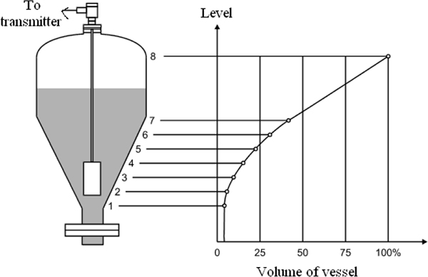
Volume measurement: entering a characteristic curve
4.3.2 Differential
When the surface pressure on the liquid is greater (as may be the case of a pressurised tank) or different to the atmospheric pressure, then a differential pressure sensor is required. This is because the total pressure will be greater than the head of liquid pressure. With the differential pressure sensor, the pressure on the surface of the liquid will be subtracted from the total pressure, resulting in a measurement of the pressure due to the height of the liquid.
In applying this method of measurement, the LP (low-pressure) side of the transmitter is connected to the vessel above the maximum liquid level. This connection is called the dry leg. The pressure above the liquid is exerted on both the LP and HP (high-pressure) sides of the transmitter, and changes in this pressure do not affect the measured level. Figure 4.4 shows differential pressure method of level measurement.
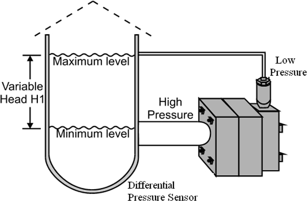
For a pressurized tank, the level is measured using differential pressure methods
Using DP (Differential pressure) for filters
Differential pressure measurement for level in pressurised tanks is also used in filters to indicate the amount of contamination of a filter. If the filter remains clean, there is no significant pressure difference across the filter. As the filter becomes contaminated, the pressure on the upstream side of the filter will become greater than on the downstream side.
Advantages
- Level measurement in pressurised or evacuated tank
- Simple to adjust
- Reasonably accurate
Disadvantages
- Dependent on relative density of material
- Quite expensive for differential pressure measurement
- Inaccuracies due to build-up
- Maintenance intensive
Application Limitations
The density of the fluid affects the accuracy of the measurement. DP instruments should be used for liquids with relatively fixed specific gravity. Also the process connections are susceptible to plugging from debris, and the wet leg of the process connection may be susceptible to freezing.
4.3.3 Bubble tube method
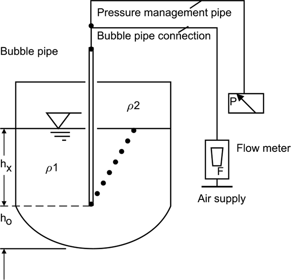
In the bubble type system, liquid level is determined by measuring the pressure required to force a gas into a liquid at a point beneath the surface.
This method uses a source of clean air or gas and is connected through a restriction to a bubble tube immersed at a fixed depth into the vessel. The restriction reduces the airflow to a very small amount. As the pressure builds, bubbles are released from the end of the bubble tube. Pressure is maintained as air bubbles escape through the liquid. Changes in the liquid level cause the air pressure in the bubble tube to vary. At the top of the bubble tube is where a pressure sensor detects differences in pressure as the level changes.
Most tubes use a small V-notch at the bottom to assist with the release of a constant stream of bubbles. This is preferable for consistent measurement rather than intermittent large bubbles. Figure 4.5 shows level measurement by using bubble tube method.
Bubble tube method
Air bubbler tube notch variations
Bubblers are simple and inexpensive, but not extremely accurate. They have a typical accuracy of about 1-2%. One definite advantage is that corrosive liquids or liquids with solids can only do damage to the inexpensive and easily replaced pipe. They do however introduce a foreign substance into the fluid.
Although the level can be obtained without the liquid entering the piping, it is still possible to have blockages. However, blockages can be minimised by keeping the pipe tip 75mm from the bottom of the tank.
Advantages
- Simple assembly
- Suitable for use with corrosive fluids.
- Intrinsically safe
- High temp applications
Disadvantages
- Requires compressed air and installation of air lines
- Build-up of material on bubble tube not permissible
- Not suited to pressurised vessels
- Mechanical wear
Application Limitations
Bubble tube devices are susceptible to density variations, freezing and plugging or coating by the process fluid or debris. The gas that is used can introduce unwanted materials into the process as it is purged. Also the device must be capable to withstand the maximum air pressure imposed if the pipe becomes blocked. Roding to clean the pipe is assisted by installing a tee section.
4.3.4 Diaphragm box
The diaphragm box is primarily used for water level measurement in open vessels. The box contains a large amount of air, which is kept within a flexible diaphragm. A tube connects the diaphragm box to a pressure gauge.
The pressure exerted by the liquid against the volume of air within the box represents the fluid pressure at that level. The pressure gauge measures the air pressure and relates the value to fluid level.
There are two common types of diaphragm boxes – open and closed. The open diaphragm box is immersed in the fluid within the vessel. The closed diaphragm box is mounted externally from the vessel and is connected by a short length of piping. The open box is suitable for applications of suspended material, and the closed type is best suited to clean liquids only. Figure 4.7 shows level measurement by using diaphragm.
Diaphragm box measurements
There are also distance limitations depending on the location of the gauge.
Advantages
- Relatively simple, suitable for various materials and very accurate
Disadvantages
- Requires more mechanical equipment, particularly with pressure vessels
4.3.5 Weighing method
This indirect type of level measurement is suited for liquids and bulk solids. Application involves using load cells to measure the weight of the vessel. With knowledge of the relative density and shape of the storage bin, the level is easy to calculate. Figure 4.8 shows level measurement by using weight.
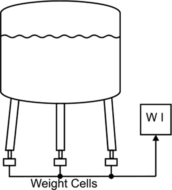
Level Measurement Using Weight
Advantages
- Very accurate level measurement for material of constant relative density
Disadvantages
- Requires a large amount of mechanical equipment
- Very costly
- Relies on consistent relative density of material
Application Limitations
A large amount of mechanical equipment is required for the framework, and is also needed to stabilise the bin.
Measurement resolution is reduced because priority is given to the accuracy of the overall weight. Unstable readings occur when the bin is being filled or emptied. Because the overall weight is the sum of both the product and container weights wind loading can cause significant problems. For these reasons most installations use a four-load cell configuration
4.4 Ultrasonic measurement
4.4.1 Principles of operation
Ultrasonic level sensors work by sending sound waves in the direction of the level and measuring the time taken for the sound wave to be returned. As the speed of sound is known, the transit time is measured and the distance can be calculated.
Ultrasonic measurement generally measures the distance between the contents and the top of the vessel. The height from the bottom is deduced as the difference between this reading and the total height of the vessel. Ultrasonic measurement systems are available that can measure from the bottom of the vessel when using liquid. Figure 4.9 shows ultrasonic level measurement.
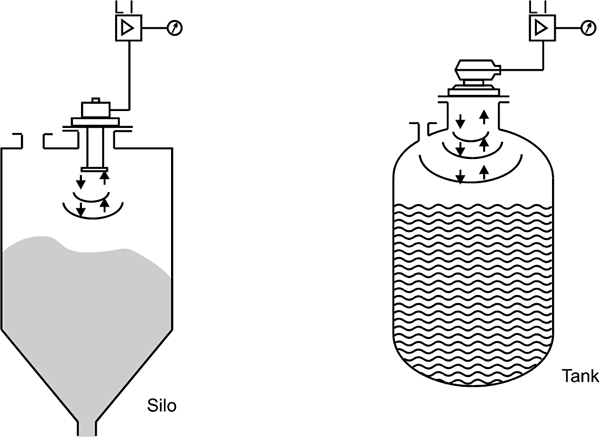
Ultrasonic measurement
The original sound wave pulse has a transmission frequency between 5 and 40 kHz; this depends on the type of transducer used. The transducer and sensor consist of one or more piezoelectric crystals for the transmission and reception of the sound signal. When electrical energy is applied to the piezoelectric crystals, they move to produce a sound signal. When the sound wave is reflected back, the movement of the reflected sound wave generates an electrical signal; this is detected as the return pulse. The transit time is measured as the time between the transmitted and return signals.
4.4.2 Selection and sizing
Below are listed some typical manufacturer’s options.
Automatic Frequency Adaption
Optimum transmission relies on a certain resonance frequency, which is dependent on the transmitter and application. This resonant frequency is also dependent on the build-up of dust, condensation or even changes in temperature.
The sensor electronics can measure the free resonant frequency during the current ringing of the membrane and changes the frequency of the next transmitted pulse to achieve an optimum efficiency.
Exact design specifications depend upon the manufacturer. Some manufacturers may vary the pulse rate and/or the gain (power).
As a guide, the transducer frequency should be chosen so that the acoustic wavelength exceeds the granule size (median diameter) by at least a factor of four. Table 4.1 shows acoustic wavelength in air verses frequency in different temperatures.
| Frequency (kHz) | Length (mm) at 0 Degree Centigrade | Length (mm) at 100 degree centigrade |
|---|---|---|
| 5 | 66 | 77 |
| 10 | 33 | 39 |
| 20 | 17 | 19 |
| 30 | 11 | 13 |
| 40 | 8 | 10 |
Spurious Echo Suppression
Although ultrasonic can produce a good signal for level, they also detect other surfaces within a vessel. Other objects that can reflect a signal can be inlets, reinforcement beams or welding seams. To prevent the device reading these objects as a level, this information can be suppressed. Even though a signal may be reflected from these objects, their characteristics will be different. Suppression of these false signals is based on modifying the detection threshold.
Most suppliers have models that map the bin and the digital data is stored in memory. The reading is adjusted accordingly when a false echo is detected.
Volume Measurement
Most modern ultrasonic measurement devices also calculate volume. This is quite simple if the vessel has a constant cross sectional area. More complex, varying cross sectional area vessels require shapes of known geometry to calculate vessel volume. Conical or square shapes with tapering near the bottom are not uncommon.
Selection considerations: The selection of ultrasonic devices should be based on the following requirement:
- Distance to be measured
- Surface of material
- Environmental conditions
- Acoustic noise
- Pressure
- Temperature Gas
- Mounting
- Self-cleaning
Advantages
- Non contact with product
- Suitable for wide range of liquids and bulk products
- Reliable performance in difficult service
- No moving parts
- Measurement without physical contact
- Unaffected by density, moisture content or conductivity
- Accuracy of 0.25% with temperature compensation and self-calibration
Disadvantages
- Product must give a good reflection and not absorb sound
- Product must have a good distinct layer of measurement and not be obscured by foam or bubbling.
- Not suitable for higher pressures or in a vacuum
- Special cable is required between the transducer and electronics
- The temperature is limited to 170°C
4.5 Electrical measurement
4.5.1 Conductive level detection
Basis of Operation
This form of level measurement is primarily used for high and low level detection. The electrode or conductivity probe uses the conductivity of a fluid to detect the presence of the fluid at the sensing location. The signal provided is either on or off.
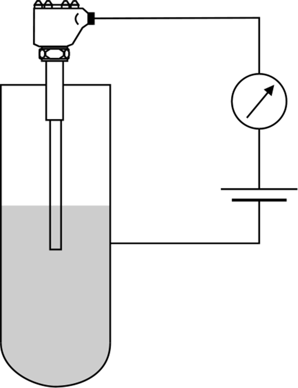
When the fluid is not in contact with the probe, the electrical resistance between the probe and the vessel will be very high or even infinite. When the level of the fluid rises to cover the probe and complete the circuit between the probe and the vessel, the resistance in the circuit will be reduced. Figure 4.10 shows conductive level detection.
Probes used on vessels constructed of a non-conductive material must have a good earth connection. The earth connection does not need to be an earthing wire it could be a feed pipe, mounting bracket or a second probe.
Corrosion of the electrode can affect the performance of the probe. Direct current can cause oxidation as a result of electrolysis, although this can be minimised by using AC power.
Conductive level detection
For level control, as opposed to level detection, two probes can be used. There are many different types of probes available. In the case of liquids that leave a residual coat on the probe, a low resistance version is required. This version is capable of detecting the difference between the actual product when the probe is immersed and a residual resistance when the probe is exposed. Such applications for this type of sensor are products, which froth, such as milk, beer or carbonated drinks.
Some of the disadvantages with conductivity switches are that they only work with conductive and non-adhesive fluids. Also in intrinsically safe applications, where sparking is not permissible, the sensors must operate at very low power. Conductivity switches are low cost and simple in design. They are a good indication for protection on pumps in the case of dry running detection.
Selection and Sizing
In assessing the application for a conductivity probe, a small AC voltage from a transformer can be applied to a metal rod to simulate the probe and the vessel wall. For accuracy, this needs to be at the same position and distance from the wall as the probe. Then with about 50mm of the rod immersed in the fluid, the current can be measured and the resistance calculated:
R in ohms = V in volts / I in amps
If the calculated resistance is less than that required for the instrument, then a conductivity probe and amplifier can be used. This is not a highly accurate means of determining the suitability; however it does give a reasonable indication. Problems with this test vary as it depends on the surface area of contact and the location of the probe.
Advantages
- Very simple and inexpensive
- No moving parts
- Good for dual point control (level switching control) in one instrument
- Good for high pressure applications
Disadvantages
- Contamination of probe with adhering materials can affect results
- Limited application for products of varying conductivity
- Intrinsic safety designs need to be specified if required
- Restricted to conductive and non coating processes
- Possible electrolytic corrosion
Application Limitations
One of the main limitations is that the liquid needs to be conductive. The manufacturer specifies the required conductivity level. A typical figure for effective operation would be below 108 ohm/cm resistivity.
Problems may arise when detecting liquid that is being agitated or is turbulent. Due to the low cost of this type of measurement, it may be desirable to install two probes to detect the same level. Alternatively, a small vertical distance between the two probes can be used to provide a dead band or neutral zone. This can protect against cycling should splashing occur (a time delay serves the same purpose).
4.5.2 Field effect level detection
Whereas the conductive probe relies on the conductivity of the fluid, the field effect probe relies on the fluid (or material) having electrical properties different to air (or the void medium).
The field effect probe produces a field between the metallic cap and the metallic gland. The metallic cap is located at the end of the probe, with the gland about 200mm away at the mounting into the vessel.
When a liquid, slurry or even solid material breaks the field, the high frequency current increases and triggers the switch. Figure 4.11 shows field effect level switch and its installation.
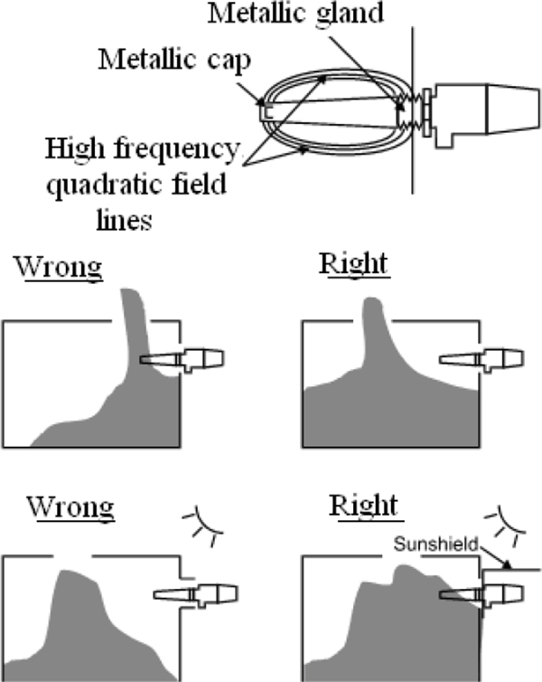
Field effect level switch and its installation (courtesy of Endress & Hauser Inc.)
Advantages and disadvantages are similar to those for the conductivity probe with the following differences:
Advantages
- Suitable for conductive or non-conductive applications
Disadvantages
- Limited in high pressure and temperature applications
Application Limitations
Due to the added expense, with only a limited number of advantages, only a few manufacturers use this technology in their products.
4.5.3 Capacitive level measurement
Basis of Operation
Capacitive level measurement takes advantage of the dielectric constant in all materials to determine changes in level. The dielectric, in terms of capacitance, is the insulating material between the plates of the capacitor. The dielectric constant is a representation of a materials insulating ability.
Quite simply, a capacitor is no more than a pair of conductive electrodes with a fixed spacing and dielectric between them. Capacitance is not limited to plates, and can be measured between probes or any other surface connected as an electrode. When a probe is installed in a vessel, a capacitor is formed between the probe and the wall of the vessel. The capacitance is well defined for many materials, and is quite low when the probe is in air. When the material covers the probe, a circuit is formed consisting of a much larger capacitance and a change in resistance. It is the changes in the dielectric constant that affects the capacitance and is ultimately what is measured. Figure 4.12 shows Simplified circuit diagram of capacitance measurement with fully insulated probes.
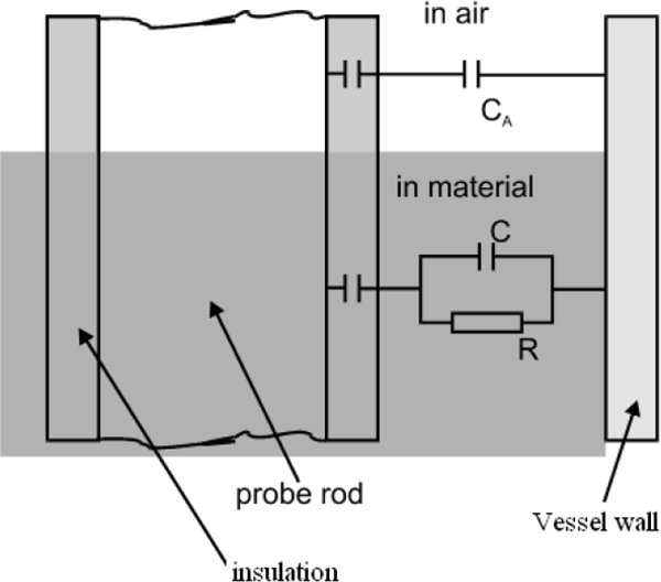
Simplified circuit diagram showing capacitance measurement with fully insulated probes
An alternative to this is the measurement of capacitance between two probes (electrodes).
Simple capacitive measurement is generally performed on non-conductive process material. In sizing an application for suitability, one of the concerns is the conductivity of the material. Problems arise when using a conductive material as this connects the plates together (an electrical short). As capacitance relies on the insulation (or dielectric), the ability to measure capacitance is impaired.
In conductive applications, the process material is grounded by its contact with the vessel wall. The only insulation (or dielectric) is the insulation on the capacitive probe. As such, the rising process material does not increase the capacitance by inserting itself between the plates as in the case of a non-conductive material. However, it increases capacitance by bringing more of the ground plate in contact with the probe insulation.
The added advantage of this type of measurement, is that not only is the capacitance measurable, but also simplified because the measurement is independent of the dielectric constant of the process material.
Selection and Sizing
Non-conductive process materials would include hydrocarbons, oils, alcohols, dry solids or similar. Process fluids that are water-based and acids can be considered as conductive.
If the conductivity exceeds a specific low threshold, then any changes in the area between the probe and the wall will not be detected. A useful numerical criterion is that materials with a relative dielectric constant of 19 or more, or a conductivity of 20 micro ohms or more, may be considered conductive. If uncertain, the process material should be considered as being conductive.
For conductive applications, the capacitive probe will need to be insulated. This is typically done with Teflon.
Screening on the probe prevents build-up of material or condensation in the vicinity of the process connection. Probes that have active build-up compensation for limit switching cancel out the effects of builds-up on the probe.
There are a number of versions of probe designs that account for conductivity and build-up. Figure 4.13 shows different Probe versions. Below is a list of some of the advantages when selecting a particular probe type:
- Probe without ground tube
- For conductive liquids
- For high viscosity liquids
- For bulk solids
- Probe with ground tube
- For non-conductive liquids
- For use in agitator vessels
- Probe with screening
- For long nozzles
- For condensation on the roof of the vessel
- For build-up on the vessel wall
- Probe with fully insulated screening
- Extra protection especially for corrosive materials
- Probe with active build-up compensation for limit detection
- For conductive build-up on the probe
- Probe with gas tight gland
- For liquefied gas tanks (if required)
- Prevents condensation forming in the probe under extreme temperature changes
- Probe with temperature spacer
- For higher operating temperatures
Probe versions
Typical Applications
Capacitive level measuring instruments are used for level detection in silos, tanks and bunkers, for both limit detection and continuous measurement. These instruments are typically used in all areas of industry and are capable of measuring liquids as well as solid materials.
Advantages
- Highly suitable for liquids and bulk solids
- No moving parts
- Suitable for highly corrosive media
Disadvantages
- Limited in its application for products of changing electrical properties (especially moisture content)
Application Limitations
Generally, capacitance level systems require calibration after installation, although some exceptions do exist.
They are limited in applications where levels of foam or other process materials with air bubbles occur.
4.6 Density measurement
Density is defined as the mass per unit volume. Specific gravity is a unit less measurement. It is the ratio of the density of a substance to the density of water, at a standard temperature. This term is also referred to as the relative density.
The measurement and control of liquid density can be quite critical in industrial processes. Density measurement gives useful information about composition, concentration of chemicals or of solids in suspension.
Density can be measured in a number of similar ways to level
- Hydrostatic pressure
- Radiation
- Vibration
- Differential pressure
The Coriolis mass flow meter is also capable of performing density measurement.
4.6.1 Hydrostatic pressure
This type of density measurement relies on a constant height of liquid and measures the pressure differences. Since level may vary, the principle of operation works on the difference in pressure between any two fixed elevations below the surface. Because the height between these two points does not change, any change in pressure is due to density variations. The distance between these points is equal to the difference in liquid head pressure between these elevations. Figure 4.14 shows fixed heights of liquid for density measurement.
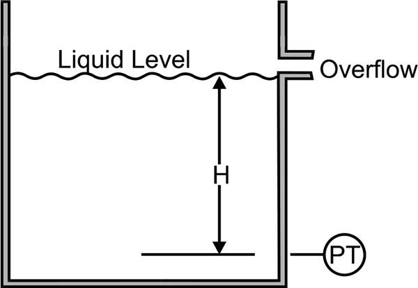
Fixed heights of liquid for density measurement
4.6.2 Radiation
Density measurement by radiation is based on the increased absorption of gamma radiation for an increase in specific gravity of the material being measured. The main components of such a system are a constant gamma source (usually radium) and a detector. Variations in radiation passing through a fixed volume of flowing liquid are converted into a proportional electrical signal by the detector.
This type of measurement is often used in dredging where the density of the mud indicates the effectiveness of the dredging vessel.
4.6.3 Vibration
Damping of a vibrating object in a fluid will increase as the density of the fluid increases. An object is vibrated from an external energy source. The object may be an immersed reed or plate.
Density is measured from one of two procedures:
- Changes in the natural frequency of vibration can be measured when the object is energised constantly
- Changes in the amplitude of vibration can be measured when the object is struck periodically, like a bell
4.6.4 Differential pressure
Constant level overflow tanks are the simplest for measuring, as only one differential pressure transmitter is required. However applications with level or static pressure variations require compensation. Figure 4.15 shows open or closed tank with varying level or pressure for level measurement.
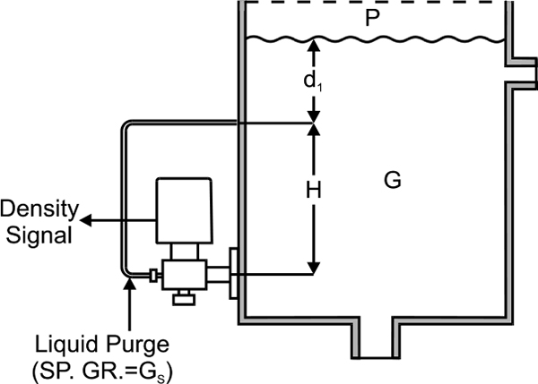
In an open or closed tank with varying level or pressure, a wet leg can be filled with seal fluid heavier than the process liquid.
Temperature Effects
Increases in temperature cause expansion of a liquid, altering its density. Not all liquids expand at the same rate. A specific gravity measurement must be corrected for temperature effects in order to be completely accurate in terms of reference conditions for density and concentration, although in most cases this is not practical.
In applications where specific gravity is extremely critical, it is possible to control the temperature to a constant value. The necessary correction to the base temperature can then be included in the density instrument calibration.
In this chapter we will discuss the principles of temperature measurements and temperature measuring devices such as thermocouples, Resistance temperature detectors (RTDs) and thermistors with their operations are highlighted.
Learning objectives
- Principles of temperature measurement
- Thermocouples
- RTDs
- Thermistors
5.1 Principles of temperature measurement
Temperature measurement relies on the transfer of heat energy from the process material to the measuring device. The measuring device therefore needs to be temperature dependent.
There are two main industrial types of temperature sensors:
- Contact
- Non contact
Contact: Contact is the more common and widely used form of temperature measurement. The three main types are:
- Thermocouples
- RTDs
- Thermistors
These types of temperature devices all vary in electrical resistance for temperature change. The rate and proportion of change is different between the three types, and also different within the type classes.
Another less common device relies on the expansion of fluid up a capillary tube. This is where the bulk of the fluid is exposed to the process materials temperature.
Many of the contact devices are not actually placed into the process – instead they are placed in a thermo well.
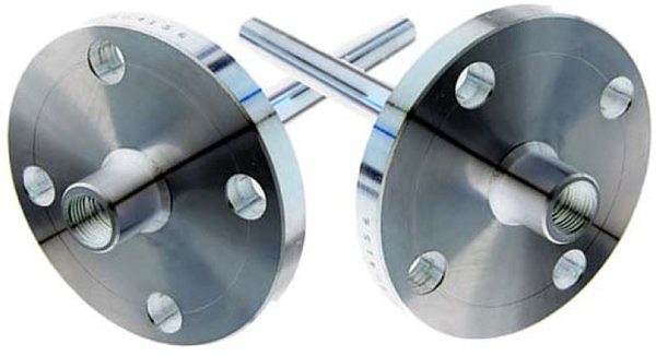
Two flanged thermo wells
The energy in the process is transferred from the fluid, through the thermo well wall, through the air gap between the thermo well and the contact temperature device, to the contact temperature device. For this reason, temperature measurement is very slow to respond to changes, and can be a problem for control applications.
Non-Contact: Temperature measurement by non-contact means is more specialized and can be performed with the following technologies:
- Infrared
- Acoustic
5.2 Thermocouples
A thermocouple is two wires of dissimilar metals that are electrically connected at one end (measurement junction) and thermally connected at the other end (the reference junction). This is shown in Figure 5.2 below. Its operation is based on the principle that temperature gradients in electrical conductors generate voltages in the region of the gradient.
Different conductors will generate different voltages for the same temperature gradient. Therefore, a small voltage, equal to the difference between the voltages generated by the thermal gradient in each of the wires (V = VA – VB), can then be measured at the reference junction.
Note that this voltage is produced by the temperature gradient along the wires and not by the junction itself. As long as the conductors are uniform along their lengths, then the output voltage is only affected by the temperature difference between the measurement (hot) junction and tile reference (cold) junction, and not the temperature distribution along the conductor between them.
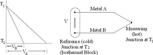
Thermocouple measurement
5.3 Resistance temperature detectors (RTDs)
5.3.1 Characteristics of RTDs
Resistance temperature detectors (RTDs) are temperature sensors generally made from a pure (or lightly doped) metal whose resistance increases with increasing temperature (positive resistance temperature coefficient).
Most RTD devices are either wire wound or metal film. Wire wound devices are essentially a length of wire wound on a neutral core and housed in a protective sleeve. Metal film RTDs are devices in which the resistive element is laid down on a ceramic substrate as a zig-zag metallic track a few micrometers thick. Laser trimming of the metal track precisely controls the resistance. The large reduction in size with increased resistance that this construction allows, gives a much lower thermal inertia, resulting in faster response and good sensitivity. These devices generally cost less than wire wound RTDs.
The most popular RTD is the platinum film PT100 (DIN 43760 Standard), with a nominal resistance of 100 Ω ± 0.1 Ω at 0°C. Platinum is usually used for RTDs because of its stability over a wide temperature range (–270°C to 650°C) and its fairly linear resistance characteristics. Tungsten is sometimes used in very high temperature applications. High resistance (1000 Ω) nickel RTDs are also available. If the RTD element is not mechanically stressed (this also changes the resistance of a conductor), and is not contaminated by impurities, the devices are stable over a long period, reliable and accurate.
5.3.2 Linearity of RTDs
In comparison to other temperature measuring devices such as thermocouples and thermistors, the change in resistance of an RTD with respect to temperature is relatively linear over a wide temperature range, exhibiting only a very slight curve over the working temperature range. Although a more accurate relationship can be calculated using curve fitting. Since the error introduced by approximating the relationship between resistance and temperature as linear is not significant, manufacturers commonly define the temperature coefficient of RTDs, known as alpha (α), by the expression:
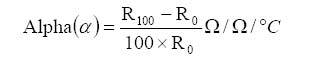
Where:
R0 = Resistance at 0°C
R100 = Resistance at 100°C
This represents the change in the resistance of the RTD from 0°C to 100°C, divided by the resistance at 0°C, divided by 100°C.
From the expression of alpha (α) it is easily derived that the resistance RT of an RTD, at temperature T can be found from the expression:
RT=R0 (l+αT)
Where:
R0= Resistance at 0°C
For example, a PT100 (DIN 43760 Standard), with nominal resistance of 100 Ω ± 0.1 Ω at 0°C has an alpha (α) of 0.00385 Ω / Ω / °C. Its resistance at 100°C will therefore be 138.5 Ω.
5.3.3 Measurement circuits and considerations for RTDs
Two-wire RTD measurement: Since the RTD is a passive resistive device, it requires an excitation current to produce a measurable voltage across it. Figure 5.3 shows a two-wire RTD excited by a constant current source, IEX and connected to a measuring device.
Two –wire RTD measurement
Any resistance, RL, in the lead wires between the measuring device and the RTD will cause a voltage drop on the leads equal to (RL × IEX ) volts. The voltage drop on the wire leads will add to the voltage drop across the RTD, and depending on the value of the lead wire resistance compared to the resistance of the RTD, may result in a significant error in the calculated temperature.
Consider an example where the lead resistance of each wire is 0.5 Ω. For a 100 ω RTD with an alpha (α) of 0.385 Ω / °C, the lead resistance corresponds to a temperature error of 2.6°C (l .0 Ω / 0.385 Ω / °C).
This indicates that if voltage measurements are made using the same two wires which carry the excitation current, the resistance of the RTD must be large enough, or the lead wire resistances small enough, that voltage drops due to the lead wire resistances are negligible. This is usually true where the leads are no longer than a few (<3) meters for a 100 Ω RTD.
5.3.4 Four-wire RTD measurement
A better method of excitation and measurement, especially when the wire lead lengths are greater than a few meters in length, is the four-wire RTD configuration shown in Figure 5.4.
Four-wire RTD measurements
RTDs are commonly packaged with four (4) leads, two current leads to provide the excitation current for the device, and two voltage leads for measurement of the voltage developed. This configuration eliminates the voltage drops caused by excitation current through the lead resistances (RL1 and RL4). Since negligible current flows in the voltage lead resistances, (RL2 and RL3) only the voltage drop across the resistance RT of the RTD is measured.
5.3.5 Three – wire RTD measurement
A reduction in cost is possible with the elimination of one of the wire leads. In the three wire configuration shown in Figure 5.5, only one lead RL1 adds an error to the RTD voltage measured.
Three-wire RTD measurements
Self-heating: Another consequence of current excitation of the RTD is the possible effect that internal heating of the device may have on the accuracy of the actual temperature measurements being made. The degree of self-heating depends on the medium in which the RTD is being used, and is typically specified as the rise in temperature for each mW of power dissipated for a given medium (i.e. still air). For a PT100 RTD device, the self-heating coefficient is 0.2°C/mW in still air, although this will vary depending on the construction of the RTD housing and its thermal properties. With an excitation current of 0.75 mA the power to be dissipated by the device is 56 μW [(0.75 × 10⁻³)2 × 100] corresponding to a rise in the temperature of the device due to self-heating of 0.011°C (56 μW × 0.2). Inaccuracies in the temperature measurement due to self-heating problems can be greatly reduced by:
- Minimizing the excitation power
- Exciting the RTDs only when a measurement is taken
- Calibrating out steady state errors
5.4 Thermistors
A cheap form of temperature sensing is provided by the thermistor, which is a thermally sensitive semiconductor resistor formed from the oxides of various metals. The type and composition of the semiconductor oxides used (i.e. manganese, nickel, cobalt etc) depend on the resistance value and temperature coefficient required.
More commonly used thermistor devices exhibit a negative temperature coefficient and have a high degree of sensitivity to small changes in temperature, typically 4% / °C.
Their accuracy is typically ten times better than thermocouples but not as accurate as RTDs. Thermistors are non-linear devices and directly useful over typical temperature ranges of –80°C up to 250°C. With regard to this, modern microprocessor based systems (either PCs or stand-alone data loggers) can be used to relieve some of the limitations caused by non-linearities, by modelling the non-linearities with quadratic equations.
Thermistors exhibit a high resistance, typically 3 kΩ, 5 kΩ, 6 kΩ and 10 kΩ at 25°C, although values as low as 100 Ω are available. High resistance means that the lead resistances of wires used to excite thermistors are usually negligible, requiring only two wire measurement schemes.
One of the attractions of thermistors is the wide range of shapes in the form of beads, discs, rods and probes that can be easily manufactured. Their small size means they have a fast thermal response, but can be quite fragile compared to RTDs (Resistance Temperature Detector) that are more robust. Just as excitation currents for RTDs can cause self-heating problems, this is even more the case for thermistors due to the higher device resistance values.
Self-heating problems can be greatly reduced by:
- Minimizing the excitation power
- Exciting the RTDs only when a measurement is taken
- Calibrating out steady state errors. Some authorities state that the temperature rise, in °C, due to self-heating can be calculated by dividing the proposed internal power dissipation by 8mW
Learning objectives
- Principles of flow measurement
- Open channel flow measurement
- Oscillatory flow Measurement
- Magnetic flow measurement
- Positive displacement
- Ultrasonic flow measurement
- Mass flow measurement
6.1 Principles of flow measurement
6.1.1 Types of flow
There are four main types of liquid flow, as shown in Table 6.1.
Table 6.1
Main types of liquid flow
| Type of flow | Notable characteristics | Process material |
| General | Thin, clean liquids | Water, light oils and solvent |
| Two-phase flow | Liquids with bubbles | Beer, wet steam, unrefined petroleum |
| Non- Newtonian | Heavy thick liquids | Grease, Paint, honey |
6.1.2 Basic terms and concepts
Laminar versus turbulent flow: In laminar flow, the fluid moves smoothly in orderly layers, with little or no mixing of the fluid across the flow stream. With laminar flow, changes in velocity can still exist as the friction of the wall slows the layers closest to the wall, while the flow in the centre of the pipe moves at a faster pace. This velocity change produces a parabolic streamlined flow profile. Figure 6.1 shows laminar and turbulent flow diagram.
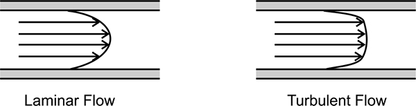
Flow profile
In turbulent flows, the laminar flow breaks down to produce intermixing between the layers. Turbulent flow is quite random, as smaller currents flow in all directions – these are also known as eddies. This type of flow has a flatter flow profile, such that the velocity of forward flow in the centre of the pipe is nearly the same as that near the walls of the pipe.
Swirl: Swirl occurs with laminar flows as fluid passes through elbows or some other form of pipeline geometry. In a similar fashion to turbulent flows, they affect the measurements of many instruments and precautions should be taken to mount measuring devices well downstream from the swirling fluid. The effects of swirls can be minimised by the use of a flow conditioner, or straightener in the line upstream.
Reynolds number: A Reynolds number defines the flow conditions at a particular point. It is a way of representing fluidity and is a useful indicator of laminar and turbulent flow. Laminar flow exists if the Reynolds number is less than 2000, and turbulence when the number is above 4000. There is not a clear transition between laminar and turbulent flows, which does complicate flow measurement in this range of operation.
The Reynolds number (Re) equation has shown below which shows the relationship between the density (ρ), viscosity (μ), pipe inside diameter (D) and the velocity (u).

Velocity: This is the speed at which the fluid passes a point along the pipe. The velocity is used to calculate volume and mass flow rates.
Volumetric flow rate: The volumetric flow rate represents that volume of fluid, which passes through a pipe per unit of time. This form of measurement is most frequently achieved by measuring the velocity of a fluid with a DP sensor as it travels through a pipe of known cross sectional area.
Mass flow rates: Mass flow is a measure of the actual amount of mass of the fluid that passes some point per unit of time
Totalized flow: Totalised flow is an accumulation of the amount of fluid that has passed a point in a pipe. This is used in both volume and mass based systems generally for accounting purposes.
Viscosity: The viscosity of a fluid defines the resistance, which the fluid has against flowing. It is typically measured in units of poise or centipoise at a given temperature. Higher numbers indicate an increase in viscosity (which is a greater resistance to flow). As the temperature of most liquids increases, their viscosity decreases and they flow more readily.
Density: The density of a fluid is the mass of the fluid per unit of volume. Density is affected by temperature and pressure variations. To avoid problems of pressure and temperature variation, mass flow measurements can be used. Although density can be of some use, it is usually more often used to infer composition, concentration of chemicals in solution or solids in suspension.
Specific Gravity: The specific gravity is the unit less ratio, found by comparing the density of a substance to the density of water at a standard temperature.
Pulsations: In maintaining good measuring conditions, pulsations in the flow stream should be recognised and avoided if possible. Common causes of pulsating flows are from pumps, compressors and two-phase fluids.
Cavitation: This condition occurs when the pressure is reduced below the vapour pressure of the liquid. This causes vapour cavities, or bubbles, to form. These bubbles can dissipate quickly causing damage to the piping system as well as the flow meter, resulting in measurement errors. Maintaining sufficient pressure in the pipe commonly solves the problem. In applications where this is likely, measurement methods requiring a pressure drop should be avoided, such as differential pressure devices.
Non-Newtonian: The normal behaviour of fluids is such that as temperature increases, viscosity decreases. There are fluids that do not abide by the standard rules of fluid dynamics. The so-called non-Newtonian fluids have viscosities that change with shear rate. Some products become thinner when agitated, whereas others stiffen when deformed.
Vena Contracta: The cross-sectional area of a fluid decreases as it is forced through a restriction. With the inertia of the fluid, the cross-sectional area continues to decrease after the fluid has passed the restriction.
Because of this, the fluids minimum cross-sectional area, which also has the maximum velocity and lowest pressure, is located at some point downstream of the restriction. This point is called the vena-contracta (as shown in Figure 6.2).
Vena-Contracta (Courtesy of Fisher Controls International)
Range ability: Range ability is the ratio of maximum to minimum flow. Range ability is used to give a relative measure of the range of flows that can be controlled.

6.1.3 Flow measurements
There are three main measurements that can be made with process flows:
- Velocity
- Volumetric flow
- Mass flow
Velocity is the speed at which the fluid moves. This by itself does not give any information about the quantity of fluid.
Volumetric flow is often deduced by knowing the cross sectional area of the fluid. Most volumetric flow equipment measures the velocity and calculates the volumetric flow based on a constant cross sectional area.

Where: v is the velocity
A is the cross sectional area
Q is the volumetric flow rate
Mass flow rate can only be calculated from the velocity or the volumetric flow rates if the density is constant. If the density is not constant, then mass flow measuring equipment is required for mass flow rate.

Where: Q is the volumetric flow rate
η is the density of the fluid
W is the mass flow rate
The flow of gases is normally measured in terms of mass per unit time. While most liquids are nearly incompressible, densities of gases vary with operating temperature and pressure. Some flow meters, such as Coriolis meters, measure the mass flow directly. Volumetric flow meters do not measure mass flow directly. Mass flow is calculated from the density and the volumetric flow as shown above. Some volumetric meters infer density based on the measured pressure and temperature of the fluid. This type of measurement is referred to as the inferred method of measuring mass flow as shown in Figure 6.3.
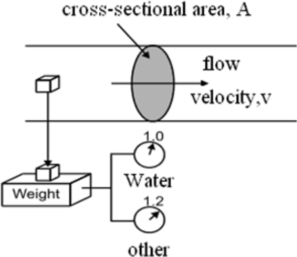
Inferred method of measuring mass flow
6.2 Open channel flow measurement
The primary devices used in open channel flow measurements are weirs and flumes.
6.2.1 Weirs
Weirs are openings in the top of a dam or reservoir that allow for the flow of liquid and enable measurement of the flow as shown in Figure 5.17. With the characteristics of the weir known, the flow is generally determined by the height of the liquid in the weir. There are two basic weirs – the rectangular and the V-notch
Rectangular
There are three types of rectangular weirs:
- Vertical walls with a flat base to form a boxlike opening in the channel
- Open weir, which extends the width of the channel
- Cippoletti weir, has the end contractions set at a 4:1 angle
V-Notch
V-notch weirs are generally metal plates that contain a V-shaped notch. The angle of the V can vary but the most common are for 30, 60 and 90 degrees.
V-notch weirs are used for lower flow rates than those that would be measured by a rectangular weir. Figure 6.4 shows rectangular, cippoletti and V-notch weirs.
Rectangular, Cippoletti and V-notch weirs
Advantages
- Simple operation
- Good Range ability (for detecting high and low flow)
Disadvantages
- Pressure loss
- Accuracy of about 2%
Application limitations: There is a high unrecoverable pressure loss with weirs, which may not be a problem in most applications. However with the operation of a weir, it is required that the flow clears the weir on departure. If the liquid is not free flowing and there is back pressure obstructing the free flow, then the level over the weir is affected and hence the level and flow measurement. Figure 6.5 shows the flow over a weir.
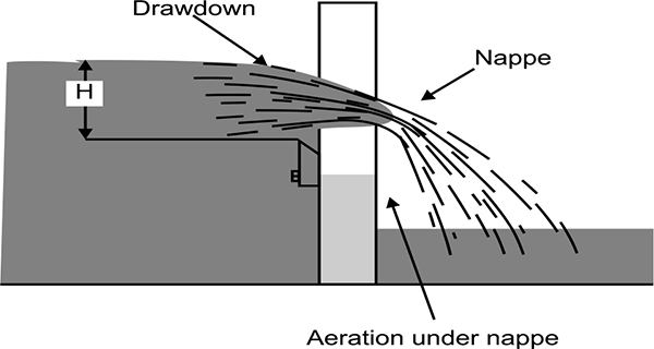
Flow over a weir
6.2.2 Flumes
Flumes are a modification to the weir where the section of flow is reduced to maintain head pressure. A flume forces the liquid into a narrower channel and in doing so only incurs a head pressure drop of about 1/4 of that for a weir of equal size. This process is similar in principle to a rectangular venturi tube.
Similar to the weir, the water level in the flume is a function of flow rate. The flume provides a little more accuracy by precisely channelling the flow. The flume is also independent of the velocity of the fluid as it enters, and as such the application does not require damming or a stilling basin. Figure 6.6 shows dimensions and diagram of flume.
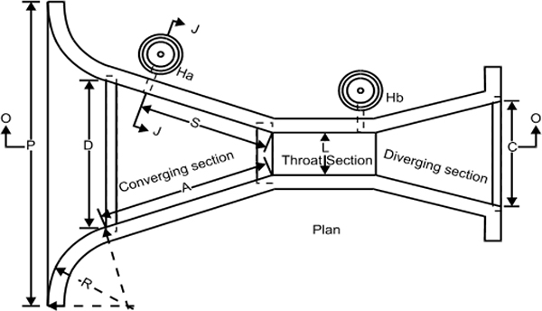
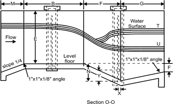
Diagram and dimensions of Parshall Flume
Typical applications: Flumes are typically used for applications involving larger scale irrigation systems, water supply, waste management and effluent treatment plants.
Advantages
- Reliable and repeatable measurements
- No erosion
- Not sensitive to dirt and debris
- Very low head pressure loss
- Simple operation and maintenance
Disadvantages
- High installation costs
- Low accuracy
- Expensive electronics
Application Limitations: Small flumes may be purchased and installed whereas larger flumes are generally fabricated on site.
6.3 Oscillatory flow measurement
Oscillatory flow equipment generally measures the velocity of flow (hence they are often referred to as velocity flow meters) and the volumetric flow rate is calculated from the relationship:

Where
Q is the volumetric flow rate
V is the velocity of the flow
A is the cross sectional area
The primary device generates a signal that is proportional to fluid velocity. This eliminates the errors that are amplified in square root calculations.
Velocity flow meters in general can operate over a greater range of velocities and are less sensitive to the flow profile compared with differential pressure devices.
6.3.1 Vortex flow meters
Vortex flow meters can measure liquid, gas or steam and use the principle of vortex shedding. Vortex shedding occurs when an obstruction is placed in the flowing stream. The obstruction is referred to as a bluff body and causes the formation of swirls, called vortices, downstream from the body. Figure 6.7 shows principle of operation of vortex meter.
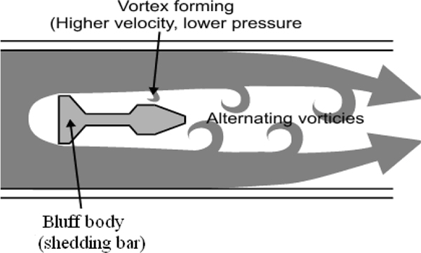
Principle of operation of vortex meter
Differential pressure changes occur as the vortices are formed and shed. This pressure variation is used to actuate the sealed sensor at a frequency proportional to the vortex shedding. For continuous flow, a series of vortices generates electrical pulses with a frequency that is also proportional to the flow velocity. The velocity can then be converted to volumetric flow rate.
The output of a vortex flow meter depends on the K-factor. The K-factor relates to the frequency of generated vortices to the fluid velocity.
The K-factor varies with the Reynolds number; however it is virtually constant over a broad range of flows. Vortex flow meters provide very linear flow rates when operated within the flat range. Figure 6.8 shows relationship between K-Factor and Reynolds number.
Relationship between K-Factor and Reynolds number
Primary Element – Bluff Bodies
Round Bluff Body: The initial bluff bodies were cylindrical and it was found that the separating point of the vortex fluctuated depending on the flow velocity. It was because of this movement that the frequency of the vortices was not exactly proportional to velocity. Figure 6.9 shows round bluff bodies.
Round bluff bodies
Delta-Shaped Bluff Body: The Delta-shaped bluff body has been tested over many years and found to be ideal in terms of its linearity. Accuracy is not affected by pressure, viscosity or other fluid conditions. Many variations of the Delta shape exist and are in operation. Figure 6.10 shows delta shaped bluff bodies.
Delta shaped bluff bodies
Two-Part Bluff Body: Applications exist where a second bluff body is inserted behind the first as shown in Figure 6.11. In this configuration, the first body is used to generate the vortices and the second body to measure them.
This method has the disadvantage of placing an extra obstruction in the stream. In such a case the pressure loss is almost doubled.
The advantage of this method is that a strong vortex is generated, which means that less complicated sensors and amplifiers may be used.
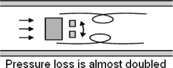
Two-part bluff body
Rectangular Bluff Bodies: One of the original bluff body designs was with a rectangular shape. This body style has been documented as unfavourable as they produce considerable fluctuations in linearity as the process density varies. Figure 6.12 shows rectangular bluff body.
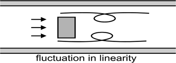
Rectangular bluff body
Vortex Swirl Type: A different type of vortex meter is that of the precession or swirl type. In this device, an internal vortex is forced into a helical path through the device. A thermistor is typically used to detect a change in temperature as the vortices pass. Again, the output signal is proportional to the flow rate. Figure 6.13 shows construction of a typical vortex precession (swirl) meter.
A flow straightener is used at the outlet from the meter. This isolates the meter from any downstream piping effects that may affect the development of the vortex.
This type of measuring device has a Ranging ability of about 10:1 and is used mainly with gases. Because of the higher tolerance in manufacture of this type of meter, it is more expensive then comparative meters.
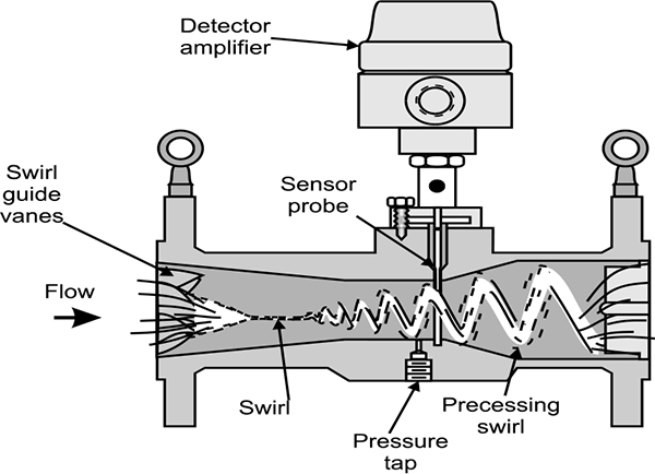
Construction of a typical vortex precession (swirl) meter
Coanda flow meter: The Coanda flow meter generates internal oscillations similar to that of an electronic oscillator. The oscillations are generated by feeding part of the mainstream flow back into itself as shown in Figure 6.14. There are two ports for feedback on opposing sides of the flow stream. The sensor (typically a thermistor) measures the frequency of oscillation, which is proportional to the rate of flow.
This flow meter has a Range ability of up to 30:1 and is used mainly with liquids.
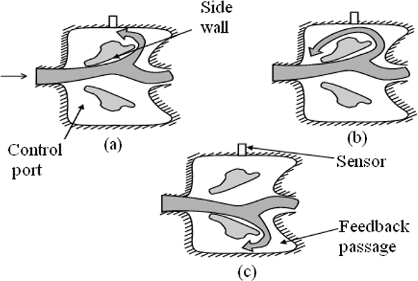
Diagram of the mode of operation of a feed back oscillator
Advantages
- Suitable for liquid, gas or steam
- Used with non-conductive fluids
- No moving parts, low maintenance
- Sensors available to measure both gas and liquid
- Not affected by viscosity, density, pressure or temperature
- Low installation cost
- Good accuracy
- Linear response
Disadvantages
- Unidirectional measurement only
- Clean fluids only
- Not suitable with partial phase change
- Not suitable for viscous liquids
- Large unrecoverable pressure drop
- Straight pipe runs required for installation
Application limitations: The upstream and downstream requirements of straight pipe vary according to a number of factors. A brief list of some of those factors is listed below:
- Severity and nature of disturbance upstream.
- Severity and nature of disturbance downstream.
- Type of Votex bluff body (the specific design of the meter).
- The accuracy required.
The nature of the disturbance can be any of the following:
- Elbow
- Regulating control valve
- Reducer
- Expander
The straight upstream and downstream lengths, required for the various installations, in order to meet stated accuracies varies between manufacturers and products. Figure 6.15 shows the pipe length requirements for installations as marketed by a particular supplier.
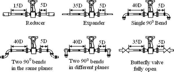
Straight pipe-run requirements as a function of upstream disturbance (Courtesy of Endress & Hauser)
Vortex flow meters are not suitable where cavitation occurs and can be damaged, but will survive flashing conditions. Flashing conditions occur when some of the incoming liquid stream is permanently vaporised in the flow meter.
6.3.2 Turbines
Basics of operation: Turbine meters have rotor-mounted blades that rotate when a fluid pushes against them. They work on the reverse concept to a propeller system. Whereas in a propeller system, the propeller drives the flow, in this case the flow drives and rotates the propeller. Since it is no longer propelling the fluid, it is now called a turbine. Figure 6.16 shows turbine flow meter.
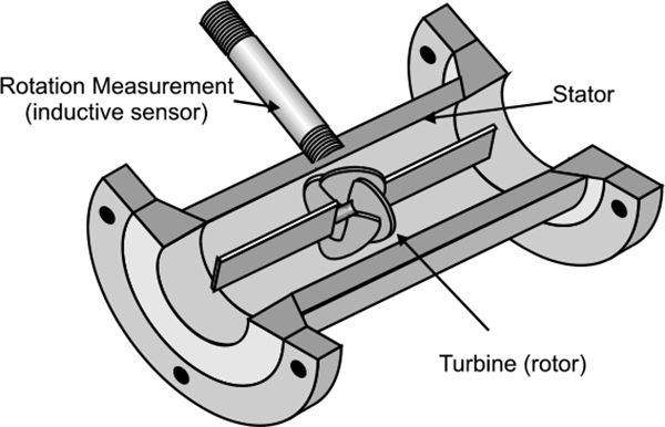
Turbine flow meter
The rotational speed of the turbine is proportional to the velocity of the fluid.
Different methods are used to convey rotational speed information. The usual method is by electrical means where a magnetic pick-up or inductive proximity switch detects the rotor blades as they turn. As each blade tip on the rotor passes the coil it changes the flux and produces a pulse. Pulse rate is directly proportional to the flow rate.
As the rotation of the turbine is measured by means of non-contact, no tapping points are required in the pipe. Pressure is therefore not a problem, and in fact pressures of up to 9300psi can be applied without any problem, but this of course does depend on pipe diameter and materials of construction.
Temperature limitations are only imposed by the limitations of the materials of construction. To reduce losses or changes in process temperature, turbine flow meters are available which can be subjected to wide temperature variations.
Turbine meters require a good laminar flow. In fact 10 pipe diameters of straight line upstream and no less than 5 pipe diameters downstream from the meter are required. They are therefore not accurate with swirling flows.
They are not recommended for use with high viscosity fluids due to the high friction of the fluid which causes excessive losses as the turbine becomes too much of an obstruction. The viscosity of the liquid must be known for use of this type of meter.
They are also subject to erosion and damage. Each meter must be calibrated for its application.
Advantages
- High accuracy, repeatability and Range ability for a defined viscosity and measuring range
- Temperature range of fluid measurement: -220oC to +350oC
- Very high-pressure capability: 9300psi
- Measurement of non-conductive liquids
- Capability of heating measuring device
- Suitable for very low flow rates
Disadvantages
- Not suitable for high viscous fluids
- Viscosity must be known
- 10 diameter upstream and 5 diameters downstream of straight pipe are required
- Not effective with swirling fluids
- Only suitable for clean liquids and gases
- Pipe system must not vibrate
- Specifications critical for measuring range and viscosity
Application limitations: As turbine meters rely on the flow, they do absorb some pressure from the flow to propel the turbine. The pressure drop is typically around 20 to 30 kPa at the maximum flow rate and does vary depending on flow rate.
While operating turbine meters sufficient line pressure is required to maintain to prevent liquid cavitation.
If the backpressure is not sufficient, then it should be increased or a larger meter chosen to operate in a lower operating range. This does have the limitation of reducing the meter flow range and accuracy.
6.4 Magnetic flow meters
Basis of operation
Electromagnetic flow meters, also known as magmeters, use Faraday’s law of electromagnetic induction to sense the velocity of fluid flow.
Faraday’s law states that moving a conductive material at right angles through a magnetic field induces a voltage proportional to the velocity of the conductive material. The conductive material in the case of a magmeter is the conductive fluid.
The fluid therefore must be electrically conductive, but not magnetic.
Magmeter
The advantages of magnetic flow meters are that they have no obstructions or restrictions to flow, and therefore no pressure drop and no moving parts to wear out. They can accommodate solids in suspension and have no pressure sensing points to block up. The magnetic flow meter measures volume rate at the flowing temperature independent of the effects of viscosity, density, pressure or turbulence. Another advantage is that many magmeters are capable of measuring flow in either direction. Figure 5.32 shows the principle of operation of the electromagnetic meter.
Most industrial liquids can be measured by magnetic flow meters. These include acids, bases, water, and aqueous solutions. However, some exceptions are most organic chemicals and refinery products that have insufficient conductivity for measurement. Also pure substances, hydrocarbons and gases cannot be measured.
In general the pipeline must be full, although with the later models, level sensing takes this factor into account when calculating a flow rate.
Magnetic flow meters are very accurate and have a linear relationship between the output and flow rate. Alternatively, the flow rate can be transmitted as a pulse per unit of volume or time.
The accuracy of most magnetic flow meter systems is 1% of full-scale measurement. This takes into account both the meter itself and the secondary instrument. Because of its linearity, the accuracy at low flow rates exceeds that of such devices as the Venturi tube. The magnetic flow meter can be calibrated to an accuracy of 0.5% of full scale and is linear throughout.
Typical applications
Magmeters are used in many applications as most liquids and slurries are suitable conductors. They are also the first to be considered in corrosive and abrasive applications. They can also be used for very low flow rates and small pipe diameters.
Advantages
- No restrictions to flow
- No pressure loss
- No moving parts
- Good resistance to erosion
- Independent of viscosity, density, pressure and turbulence
- Good accuracy
- Bi-directional
- Large range of flow rates and diameters
Disadvantages
- Expensive
- Most require a full pipeline
- Limited to conductive liquids
Application Limitations: As mentioned earlier, a magnetic flow meter consists of either a lined metal tube, usually stainless steel because of its magnetic properties, or an unlined non-metallic tube. The problem can arise if the insulating liners and electrodes of the magnetic flow meter become coated with conductive residues deposited by the flowing fluid. Erroneous voltages can be sensed if the lining becomes conductive.
Maintaining high flow rates reduces the chances of this happening. However, some manufacturers do provide magmeters with built in electrode cleaners.
Block valves are used on either side of ac-type magmeters to produce zero flow and maintain a full pipe to periodically check the zero calibration limits. DC units do not have this requirement.
6.5 Positive displacement
Positive displacement meters measure flow rate by repeatedly passing a known quantity of fluid from the high to low pressure side of the device in a pipe. The number of times the known quantity is passed gives information about the totalised flow. The rate at which it is passed is the volumetric flow rate. Because they pass a known quantity, they are ideal for certain fluid batch, blending and custody transfer applications. They give very accurate information and are generally used for production and accounting purposes.
6.5.1 Rotary vanes
Spring loaded vanes slide in and out of a channel in a rotor so that they make constant contact with the eccentric cylinder wall. When the rotor turns, a known volume of fluid is trapped between the two vanes and the outer wall. The flow rate is based on volume per revolution. Figure 6.17 shows a rotating vane meter.
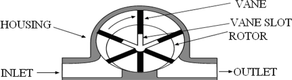
Rotating vane meter
The piston type is suitable for accurately measuring small volumes and is not affected by viscosity. Limitations with this device are due to leakage and pressure loss.
Typical applications: This type of meter is used extensively in the petroleum industry for such liquids as gasoline and crude oil metering.
Advantages
- Reasonable accuracy of 0.1%.
- Suitable for high temperature service, up to 180oC.
- Pressures up to 7Mpa.
Disadvantages
- Suitable for clean liquids only.
Lobed impeller: This type of meter uses two lobed impellers, which are geared and meshed to rotate at opposite directions within the enclosure. A known volume of fluid is transferred for each revolution. Figure 6.18 shows a rotating lobe meter.
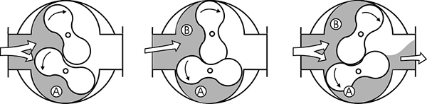
Rotating lobe meter
Typical Applications: The lobed impeller meter is often used with gases.
Advantages
- High operating pressures, up to 8Mpa.
- High temperatures, up to 200°C.
Disadvantages
- Poor accuracy at low flow rates.
- Bulky and heavy.
- Expensive.
6.5.2 Oval gear meters
Two oval gears are intermeshed and trap fluid between themselves and the outer walls of the device. The oval gears rotate due to the pressure from the fluid and a count of revolutions determines the volume of fluid moving through the device. Figure 6.19 shows the measure of flow ad volume using oval gear meters.
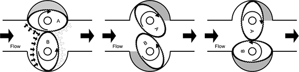
Oval gear meters for measuring volume and flow
Positive displacement meters measure volumetric flow rate directly by dividing a stream into distinct segments of known volume, counting segments and multiplying by the volume of each segment. The viscosity of the fluid can affect the leakage, or slip flow. If the meter is calibrated on a particular fluid, it will read marginally higher should the viscosity rise.
Newer designs of this type of meter use servomotors to drive the gears. This eliminates the pressure drop across the meter and also the force required driving the gear. This eliminates the force, which causes the slip flow. This mainly applies to smaller sized meters and significantly increases the accuracy at low flows.
Advantages
- High accuracy of 0.25%
- High operating pressures, up to 10MPa
- High temperatures, up to 300oC
- Wide range of materials of construction
Disadvantages
- Pulsations caused by alternate drive action
6.6 Ultrasonic flow measurement
There are two types of ultrasonic flow measurement:
- Transit time measurement
- Doppler effect
The fundamental difference is that the transit-time method should be used for clean fluids, while the Doppler reflection type used for dirty, slurry type flows.
6.6.1 Transit time
The transit-time flow meter device sends pulses of ultrasonic energy diagonally across the pipe. The transit-time is measured from when the transmitter sends the pulse to when the receiver detects the pulse Figure 6.20 shows transit time measurement.
Each location contains a transmitter and receiver. The pulses are sent alternatively upstream and downstream and the velocity of the flow is calculated from the time difference between the two directions.
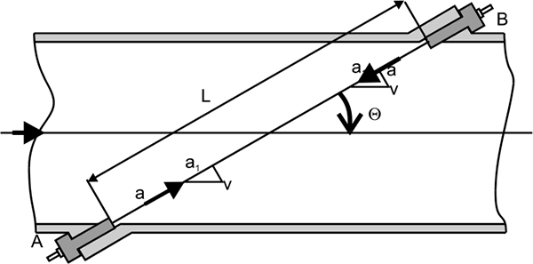
Transit time measurement
Application limitations
Clamp-on designs are limited because of the differing mediums in which the ultrasonics signals pass through. For optimum results, a sound-conductive path is required between the transducer and the process fluid inside the pipe. Couplings are available for reducing these effects but are quite expensive.
Typical applications: Transit-time ultrasonic flow measurement is suited for clean fluids. Some of the more common process fluids consist of water, liquefied gases and natural gas.
Doppler Effect: The Doppler effect device relies on objects with varying density in the flow-stream to return the ultrasonic energy. With the Doppler effect meter, a beam of ultrasonic energy is transmitted diagonally through the pipe. Portions of this ultrasonic energy are reflected back from particles in the stream of varying density. Since the objects are moving, the reflected ultrasonic energy has a different frequency. The amount of difference between the original and returned signals is proportional to the flow velocity. Figure 6.21 shows the Doppler effect.
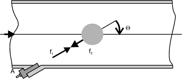
Doppler Effect
It is quite common for only one sensor to be used. This contains both the transmitter and receiver. These can also be mounted outside of the pipe.
Application limitations: As the Doppler flow meter relies on reflections from the flow stream, it therefore requires sufficiently sized solids or bubbles. It is also required that the flow be fast enough to maintain a suitable quantity of solids and bubbles in suspension. Higher frequency Doppler flow meters are available, but are limited to cleaner fluids.
Advantages
- Suitable for large diameter pipes
- No obstructions, no pressure loss
- No moving parts, long operating life
- Fast response
- Installed on existing installations
- Not affected by fluid properties
Disadvantages
- Accuracy is dependent on flow profile
- Fluid must be acoustically transparent
- Errors cause by build up in pipe
- Only possible in limited applications
- Expensive
- Pipeline must be full
Application limitations: Turbulence or even the swirling of the process fluid can affect the ultrasonic signals. In typical applications the flow needs to be stable to achieve good flow measurement, and typically allowing sufficient straight pipe up and downstream of the transducers does this. The straight section of pipe upstream would need to be 10 to 20 pipe diameters with a downstream requirement of 5 pipe diameters.
For the transit time meter, the ultrasonic signal is required to traverse across the flow, therefore the liquid must be relatively free of solids and air bubbles. Anything of a different density (higher or lower) than the process fluid will affect the ultrasonic signal.
6.7 Mass flow meters
Mass flow measurement gives a more accurate account of fluids, and is not affected by density, pressure and temperature (unlike volumetric measurements).
Although most meters can infer mass flow rate from volumetric flow measurements, there are a number of ways to measure mass flow directly:
- The Coriolis meter
- Thermal mass flow meter
- Radiation density
6.7.1 The Coriolis Meter
The Coriolis Effect: The basis of the Coriolis meter is Newtons’ Second Law of Motion, where:
Force = Mass x Acceleration.
The conventional way to measure the mass of an object is to weigh it. In weighing, the force is measured with a known acceleration (9.81m/sec2). This type of measuring principle is not easy or possible with fluids in motion, particularly in a pipe.
However, it is possible to manipulate the above formula and apply a known force and measure, instead, the acceleration to determine the mass. Figure 6.22 shows Principle of Coriolis effect.
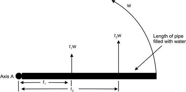
Principle of Coriolis Effect
The Coriolis Effect causes a retarding force on a rotating section of pipe when flow is moving outward, conversely producing an advance on the section of pipe for flow moving towards the axis of rotation. Figure 6.23 shows application of Coriolis force to a meter.
Application of Coriolis force to a meter
When the full section of pipe is moved about its axis in an oscillatory motion, the outgoing section of pipe is retarded (or decelerated) and the return section is advanced (or accelerated), producing a twist in the pipe.
Coriolis Meter: The force is applied to oscillate the flow pipes and the Coriolis effect is the principle used to determine the acceleration due to the torque (the amount of twisting). Sensors are used to measure the amount of twist in the flow tubes within the meter as a result of the flow tube vibration and deflection due to the mass flow. The amount of twist measured is proportional to the mass flow rate and is measured by magnetic sensors mounted on the tubes.
Developments on the looped pipe Coriolis meter were made to keep to the pipes straight. This is done by making the pipes straight and parallel. The force is applied by oscillating the pipes at the resonant frequency. This has the advantage of reducing pressure loss in the pipeline. Figure 6.24 shows Coriolis meter construction.
Coriolis meter construction
6.7.2 Thermal Mass Flow meters
The two main types of thermal mass flow measuring devices are:
- Thermal Anemometer
- Temperature rise flow meter
6.7.3 Radiation density
One of the limitations of flow meters is that they measure volumetric flow only. As mentioned previously, if the density is known and is constant, then mass flow rate can be calculated. Problems arise when the density varies.
It is however possible and quite acceptable practice to combine volumetric flow equipment with density measuring devices to obtain accurate mass flow measurements. One such combination is the use of a magmeter with a radiation densitometer.
Learning objectives
- Processes, controllers and tuning
- PID controllers
- Gain, dead time and time constants
- Process noise
- General purpose closed loop tuning method
7.1 Processes, controllers and tuning
Most basic process control systems consist of a control loop, comprising of following four main components
- A measurement of the state or process condition
- A controller used for calculating the action based on its measured value against a pre-set or desired value (Set Point)
- An output signal resulting from the controller calculation which is used to manipulate the process action form one of the actuators
- The process that itself reacts with this signal and changes its state or condition
Block diagram showing the elements of a process control loop
The most important signals used in process control are as follows:
- Process Variable (PV)
- Manipulated Variable (MV)
In industrial process control, PV is measured in the field and acts as an input to an automatic controller which takes action based on its value. Alternatively the PV can be treated as input to a data display so that the operator can use the readings in order to adjust the process through manual control and supervision.
The variable has to be manipulated, in order to get control over the PV; the value thus obtained is called the MV. For instance, if we want to control a particular flow, we manipulate a valve to control the flow. Here, the valve position is called MV and the measured flow becomes PV.
In case of a simple automatic controller, the Controller Output Signal (OP) drives the MV. In more complex automatic control systems, a controller output signal may drive the target values or reference values for other controllers.
The ideal value of the PV is often called Target Value and in the case of an automatic control, the term Set Point Value is preferred.
7.1.1 Process modelling
The process plant is represented by an input/output block as shown in Figure 7.2.
Basic block diagram for the process being controlled
From Figure 7.2 a controller signal is viewed that will operate on input to the process, known as the MV. We try to drive the output of the process to a particular value or set a point by changing the input. The output may also be affected by other conditions in the process or by external actions such as changes in supply pressures or in the quality of materials being used in the process. These are all regarded as disturbance inputs and the control action present in the system overcome’s their influences as best as possible.
The challenge for the process control designer is to maintain the controlled process variable at the target value or change it to meet production needs while compensating for the disturbances that may arise from other inputs. For example if you want to keep the level of water in a tank at a constant height while others are drawing off from it, you will manipulate the input flow to keep the level steady.
The value of a process model is providing a means to show the way the output would respond to the actions of the input. This is done by having a mathematical model based on the physical and chemical laws affecting the process. For example in Figure 7.3 an open tank with cross sectional area A is supplied with an inflow of water Q1 that can be controlled or manipulated. The outflow from the tank passes through a valve with a resistance R to the output flow Q2. The level of water or pressure head in the tank is denoted as H. We know that Q2 will increase as H increases and when Q2 equals Q1 the level will become steady.
The block diagram version of this process is drawn in Figure 7.4.
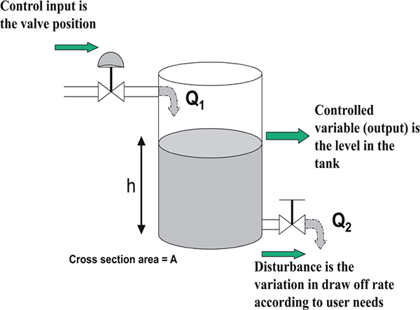
Example of a water tank with controlled inflow
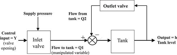
Elementary block diagram of tank process
Note that the diagram only shows the flow of variables into functional blocks and summing points so that we can identify the input and output variables for each block.
We want this model to tell us how H will change if we adjust the inflow Q1 while we keep the outflow valve at a constant setting. The model equations can be written as follows:
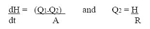
The first equation says the rate of change in level is proportional to the difference between inflow and outflow divided by the cross sectional area of the tank. The second equation says the outflow will increase in proportion to the pressure head divided by the flow resistance, R.
Cautionary Note: For turbulent flow conditions in the exit pipe and the valve, the effective resistance to flow R, will actually change in proportion to the square root of the pressure drop so we should also note that R = a constant x√ H. This creates a non-linear element in the model which makes things more complicated. However, in control modelling it is a common practice to simplify the nonlinear elements when we are studying dynamic performance around a limited area of disturbance. So for a narrow range of level we can treat R as a constant. It is important that this approximation is kept in mind because in many applications problems arise very often, when a loop tuning is being set up on the plant at conditions away from the original working point.
The process input/output relationship is therefore defined by substituting for Q2 in the linear differential equation:
dH/dt = Q1/A – H/RA
This is rearranged to a standard form as
(R.A.) (dH/dt) + H = R. Q1
When this differential equation is solved for H it gives
H = R. Q1 (1-e-t/RA)
Using this equation we can say that if a step change in flow Δ Q1 is applied to the system, the level will rise by the amount Δ Q1.R by following an exponential rise versus time. This is the characteristic of a first order dynamic process and is very commonly seen in many physical processes. These are sometimes called capacitive and resistive processes and include examples such as charging a capacitor through a resistance circuit (see Figure 7.5) and heating of a well mixed hot water supply tank (see Figure 7.6).
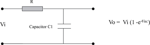
Resistance and capacitor circuit with 1st order response.
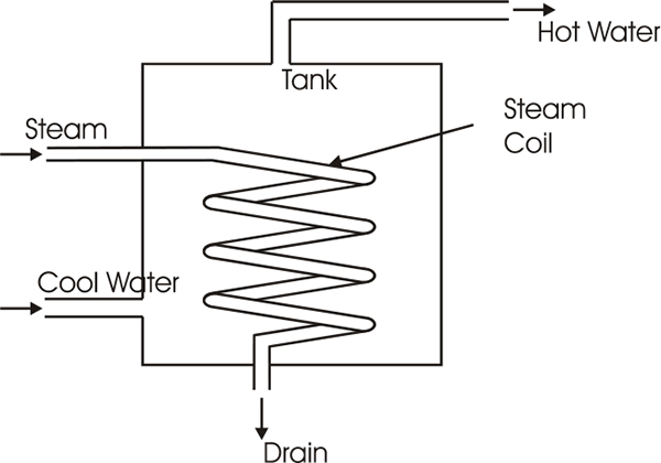
Resistance and capacitance effects in a water heater
7.1.2 Process dynamics and time constants
Resistance, capacitance and inertia are perhaps the most important effects in industrial processes involving heat transfer, mass transfer, and fluid flow operations. The essential characteristics of first and second order systems are summarized below and they may be used to identify the time constant and responses of many processes as well as mechanical and electrical systems. In particular it should be noted that most of the process measuring instruments will exhibit a certain amount of dynamic lag and this must be recognized in any of the control system applications, since it is a factor in response and in control loop tuning.
First order process dynamic characteristics
The general version of the process model for a first order lag system is a linear first order differential equation
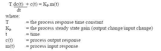
The output of a first order process follows the step change input with a classical exponential rise as shown in Figure 7.7.
Important points to note: ‘T’ is the time constant of the system and is the time taken to reach 63.2% of the final value after a step change has been applied to the system. After 4 times the constant the output response has reached 98% of the final value that it will settle.
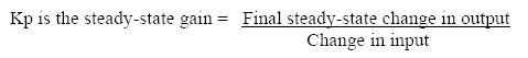
The initial rate of rise of the output will be Kp/T.
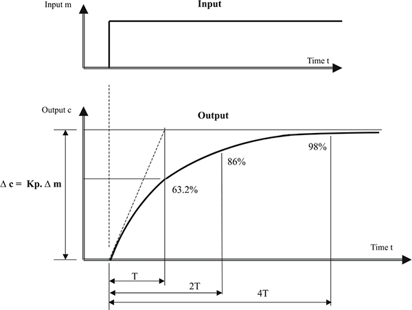
First order response
Application to the tank example
If we apply some typical tank dimensions to the response curve in figure 7.7 we can predict the time. The tank level example in Figure 7.3 will need to stabilize after a small step change around a target level H.
For example: We Suppose the tank has a cross sectional area of 2 m2 and operates at H = 2m when the outflow rate is 5m3 per hour. The resistance constant R will be H/Q2 = 2 m/5 m3 /hr = 0.4 hr/m2 and the time constant will be AR = 0.8 hrs. The gain for a change in Q1 will also be R.
Hence if we make a small corrective change at Q1 of say 0.1 m3 /hr the resulting change in level will be: R.Q1 = 1 x 0.4 = 0.4 m and the time to reach 98% of that change will be 3.2 hours.
Resistance process
As we have seen how a first order process behaves, we can summarize the possible variations that may be found by considering the equivalent of resistance, capacitance and inertia type processes.
If a process has very little capacitance or energy storage the output response to a change in input will be instantaneous and proportional to the gain of the stage. For example: If a linear control valve is used to change the input flow with reference to the tank example of Figure 7.3 the output flow will rise immediately to a higher value with a negligible lag.
Capacitance type processes
Most processes include some form of capacitance or storage capability, either for materials (gas, liquid or solids) or for energy (thermal, chemical, etc.). Those parts of the process have the ability to store mass or energy and are termed as ‘capacities’. They are characterized by storing energy in the form of potential energy, for example, electrical charge, fluid hydrostatic head, pressure energy and thermal energy.
The capacitance of a liquid or gas storage tank is expressed as area units. These processes are illustrated in Figure 7.8. The gas capacitance of a tank is constant and is analogous to electrical capacitance.
The liquid capacitance equals the cross-sectional area of the tank at the liquid surface; if this is constant then the capacitance is also constant at any head.
Using Figure 7.8 consider if we have a steady condition where flow into the tank matches the flow out via an orifice or valve with flow resistance r. If we change the inflow slightly by Δv the outflow will rise as when the pressure rises until we have a new steady state condition. For a small change we can take ‘r’ to be a constant value. The pressure and outflow responses will follow the first order lag curve as seen in Figure 7.7 and is given by the following equation:
Δp = r. Δv (1-e-t/r.C)
Here the time constant will be r.C.
It is clear that this dynamic response follows the same laws as those for the liquid tank shown in the example of Figure 7.3 and for the electrical circuit shown in Figure 7.5.
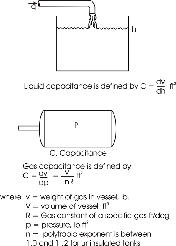
Capacitance of a liquid or gas storage tank expressed in area units
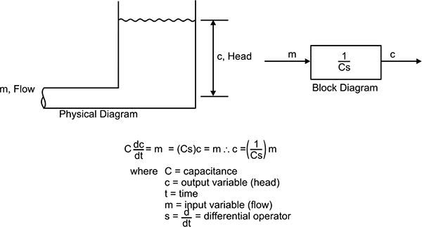
Liquid capacitance calculation; the capacitance element
A purely capacitive process element can be illustrated by a tank with only an inflow connection such as Figure 7.9. In such a process, the rate at which the level rises is inversely proportional to the capacitance and the tank will eventually flood. Initially for an empty tank with constant inflow, the level c is the product of the inflow rate m and the time period of charging t divided by the capacitance of the tank C.
Inertia type processes
Inertia effects are typically due to the motion of matter involving the storage or dissipation of kinetic energy. They are most commonly associated with mechanical systems involving moving components, but are also important in some of the flow systems in which fluids must be accelerated or decelerated. The most common example of a first-order lag caused by kinetic energy builds up when a rotating mass is required to change speed or when a motor vehicle is accelerated by an increase in engine power up to a higher speed until the wind and rolling resistances match the increased power input.
Second-order response
Second order processes result in a more complicated response curves. This is due to the exchange of energy between inertia effects and interactions between first order resistance and capacitance elements. They are described by the second order differential equation:
The solutions to the equation for a step change in m(t) with all initial conditions zero, can be any one of the family of curves as shown in Figure 7.10. There are three broad classes of responses in the solution, depending on the value of damping ratio.
- ξ < 1.0, the system is under damped and overshoots the steady-state value
- If ξ < 0.707, the system will oscillate about the final steady-state value
- ξ > 1.0, the system is over damped and will not oscillate or overshoot the final steady-state value
ξ = 1.0, the system is critically damped. In this state it yields the fastest response without overshoot or oscillation. The natural frequency of oscillation will be ωn = 1/T and is defined in terms of the ‘perfect’ or ‘frictionless’ situation where ξ = 0.0. As the damping factor increases the oscillation frequency decreases or stretches out until the critical damping point is reached.
Step response of a second order system
Important note: When a simple feedback control loop is applied to a first order system or to a second order system, the overall transfer function of the combined process and control system will usually be equivalent to a second order system. Hence the response curves shown in Figure 7.10 will be seen in typical closed loop control system responses.
Multiple time constant processes
In multiple time constant processes, say where two tanks are connected in series, the process will have two or more than two time lags operating in series. As the number of time constants increases, the response curves of the system become progressively more retarded and the overall response gradually changes into an S-shaped reaction curve as can be seen in Figure 7.11.
High order response
Any process that consists of a large number of process stages connected in series, can be represented by a set of series connected in first order lags or transfer functions. When combined for the overall process they represent a high order response but very often one or two of the first order lags will be dominant or can be combined. Hence many processes can be reduced to approximate first or second order lags but they will also exhibit a dead time or transport lag as well.
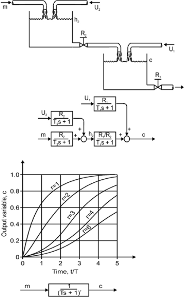
Response curves of processes with several time constants
7.2 Proportional–Integral–Derivative (PID) Controllers
A PID controller is a feedback mechanism used for the purpose of industrial control systems. The controller minimises the error by adjusting the process control inputs.
Comparative descriptions of real and ideal controllers
The Ideal PID-Controller is not suitable for direct field interaction; therefore it is called the Non-Interactive PID-Controller. It is highly responsive to electrical noise on the PV input if the derivative function is enabled.
The Real PID-Controller is especially designed for direct field interaction and therefore called the Interactive PID-Controller. Due to internal filtering in the derivative block the effects of electrical noise on the PV input is greatly reduced.
7.2.1 Ideal or non-Interactive PID controller
The Non-Interactive form of controller is the classical teaching model of PID algorithms. It gives a student a clear understanding of P, I and D control, since P-Control I-Control and D-Control can be seen independent of each other.
PID is effectively a combination of independent P, I and D-control actions. This can be seen in Figure 7.12.
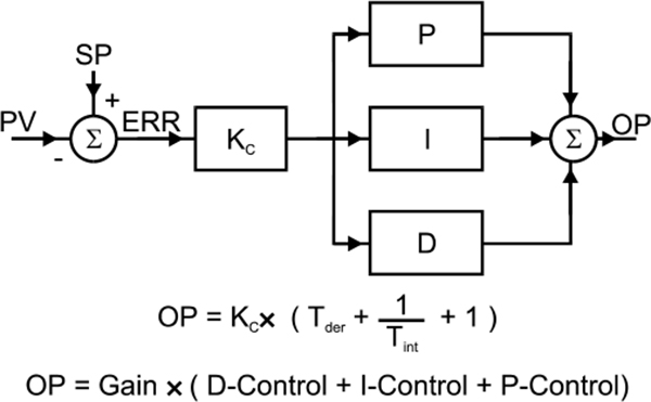
Ideal PID-controller
Since P, I and D algorithms are calculated independently in an Ideal PID-Controller, this form of controller is recommended if an ideal process variable exists.
Ideal process variables
An ideal process variable is a noise-free, refined and optimized variable. They are the result of computer optimization, process modelling, statistical filtering and value prediction algorithms. These types of ideal process variables do not come from field sensors.
In these cases, it is of great benefit that the actual formula of the Ideal PID algorithm is simple, as shown in Figure 7.13.
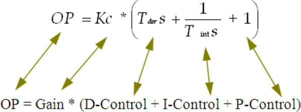
Ideal PID algorithm
7.2.2 Real or interactive PID controller
The Interactive form is the PID algorithm used for direct field control. That is either or both of its input (PV) and output (MV) are directly connected to field or process equipment. It is designed to cope with any of the electrical noise induced into its circuits by equipment in the plant or factory.
Full understanding of the Interactive PID algorithm is a difficult task, since P-Control, I-Control and D-Control cannot be seen independent from each other. Therefore, Interactive PID is not just a sum of independent P, I and D control. This can be seen in Figure 7.14.
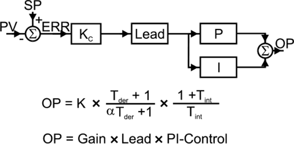
Real PID-controller
Since the Interactive PID-Controller makes use of a Lead algorithm rather than using the classical mathematical derivative, it is best suited for real (field) process variables.
Real process variables (field originated)
A real process variable has electrical noise that comes from field sensors or the connecting cables. It is therefore of great benefit that the PID algorithm has some noise reduction built in. The formula below represents an Interactive PID algorithm (see Figure 7.15).
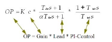
Real PID algorithm
7.2.3 Lead function – derivative control with filter
The field controller uses a Lead Algorithm for derivative control. The block diagram is shown in Figure 7.16.
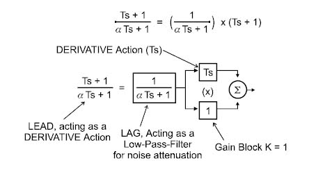
Block diagram of lead as derivative
7.3 Gain, dead time and time constants
We have discussed the different types of controllers in the previous sections. Now let us discuss about the process gain, dead time and time constant.
The process gain describes the how much the process will respond to a change in controller output, while the dead time and time constant describes how quickly the process will respond. Dead time is the times taken by the system to start responding to a process were as time constant is the fastness of the process on it is started.
7.3.1 Process gain
The process gain is the ratio of the change in the output (once it has settled to a new steady state) to the change in the input. This is the ratio of the change in the PV to the change in the MV.
It is also referred to as the process sensitivity, as it describes the degree to which a process responds to an input.
A slow process is one with low-gain, where it takes a long time to cause a small change in the MV. An example of this is home heating, where it takes a long time for the heat to accumulate to cause a small increase in the room temperature. A high gain controller should be used for such a process.
A fast process has a high gain, i.e. the MV increases rapidly. This occurs in systems such as a flow process or a pH process near neutrality where only a droplet of reagent will cause a large change in pH. For such a process, a low gain controller is needed.
The three component parts of process gain, from the controllers perspective is the product of the gains of the measuring transducer (KS), the process itself (KC) and the gain of what the PV or controller output drives (KV).
This becomes: Process Gain = KS x KC x KV
7.3.2 Dead time or transport delay and time constant
In processes involving the movement of mass, dead time is a significant factor in the process dynamics. It is a delay in the response of a process after some variable is changed, during which no information is known about the new state of the process. It may also be known as the transportation lag or time delay.
Dead time is the worst enemy of good control and every effort should be made to minimize it.
All process response curves are shifted to the right by the presence of dead time in a process (see Figure 7.17).
Once the dead time has passed, the process starts responding with its characteristic speed, called the process sensitivity.
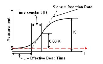
Process reaction or response curve, showing both dead time and time constant
This would be seen for example in a long pipeline if the liquid blend was changed at the input or the liquid temperature was changed at the input and the effects were not seen at the output until the travel time in the pipe has expired.
In practice, the mathematical analysis of uncontrolled processes containing time delays is relatively simple but a time delay, or a set of time delays, within a feedback loop tends to lend itself to very complex mathematics.
In general, the presence of time delays in control systems reduces the effectiveness of the controller. In well-designed systems the time delays (deadtimes) should be kept to the minimum.
7.4 Process noise
Noise is a disturbance in the input or output which may cause a major downfall in the performance of any loop.
Derivative action and effects of noise: The most important difference between Non-Interactive and Interactive PID controllers is the different impact noise has on a controller’s output. It must be remembered that derivative control multiplies noise.
Introduction to filter requirements: Both Non-Interactive PID and Interactive PID controllers make use of a noise filter for process noise (known as the process variable filter time constant TD).
Since the derivative control of a Non-Interactive PID has no noise suppression of its own, noise will always be a major problem, even though a Process Variable filter may be used.
Since the derivative control of an Interactive PID already has some noise suppression of its own, noise is not so much of a problem, and is even less if a process variable filter is used.
It is recommended that a PV filter should be used in all cases where derivative control is being used. The author has observed numerous derivative control systems having excessive movement of the controller outputs due to the lack of PV filters.
This type of problem is often incorrectly interpreted by personnel (in industrial plants) i.e. a problem of stability. Hence an important rule is to make a clear distinction between noise and instability in industrial control applications.
As discussed earlier, noise and instability require treatment with different methodologies, as they are totally different problems. Remember, a process variable filter, due to its LAG action, a reduced noise is seen but may add to loop instability.
7.5 General purpose closed loop tuning method
PID controller is a standard feedback used in industrial control applications. The output is maintained at a targeted value by controlling the input. This targeted value is called as set point. The advantage of the closed loop systems is that it can be used for tuning the controller. Here the behaviour of the system with its control, need to be studied.
7.5.1 Ziegler-Nichols (ZN) closed-loop tuning method
This tuning method is one of the most common methods. This was first introduced by J.G. Ziegler and N.B. Nichols in 1942. Most of the process control loops use this method. This method is automatically tested by a controller. This method determines the oscillatory loop gain with a proportionality control. The controller gain, reset and derivative values can be derived form the gain at which oscillations are sustained. The period of oscillation at the gain is also known. The ZN method should produce tuning parameters which will obtain quarter wave decay.
Steps to be followed:
- Make sure that the process is “lined out” with the loop to be tuned in automation with a gain sufficiently low so as to prevent oscillation
- Increase the gain in steps of 50% of the previous gain. After each step, check for the oscillation and change the set point if there are no oscillations, so as to trigger any oscillation
- Adjust the gain so that the oscillation is persistent. (If the oscillation is increasing, decrease the gain slightly. If it is decreasing, increase the gain slightly)
- Make a note of the gain which causes persistent oscillations and the period of oscillation. These are the “Ultimate Gain” (GU) and the “Ultimate Period” (PU) respectively.
- Calculate the tuning for the following set of equations. Use the set which corresponds with the desired configuration: P only, PI, or PID.
Tuning Equations
P Only: Gain = 0.5 GU
PI: Gain=0.45 GU, Reset=1.2/PU
PID: Gain=0.6GU, Reset=2/PU, Derivative=PU/8
Table 7.1
Effect of changes in parameters
| Parameter | Rise time | Overshoot | Settling time | S.S. error |
| P | Decrease | Increase | Small change | Decrease |
| I | Decrease | Increase | Increase | Eliminate |
| D | Small change | Decrease | Decrease | Small change |
In this chapter we will discuss the introduction to control valves, definition of a control valve, cavitation and flashing.
Learning objectives
- Introduction
- Definition of a control valve
- Cavitation
- Flashing
8.1 Introduction
Control valves are the essential final elements used to control fluid flow and pressure conditions in a vast range of industrial processes. The control valve industry is itself a vast enterprise whilst the influence of control valves on the performance of high value processes worldwide is very much larger. Hence it is a major responsibility on control and instrumentation engineers to deliver the best possible control valve choices for every application they encounter. The task of specifying and selecting the appropriate control valve for any given application requires an understanding of the principles of:
- How fluid flow and pressure conditions determine what happens inside a control valve
- How control valves act to modify pressure and flow conditions in a process
- What types of valves are commonly available
- How to determine the size and capacity requirements of a control valve for any given application
- How actuators and positioners drive the control valve
- How the type of valve influences the costs
Selecting the right valve for the job requires that the engineer should be able to:
- Ensure that the process requirements are properly defined
- Calculate the required flow capacity over the operating range
- Determine any limiting or adverse conditions such as cavitation and noise and know how to deal with these
- Know how to select the valve that will satisfy the constraints of price and maintainability whilst providing good performance in the control of the process
8.1.1 Purpose of control Valve
The purpose of a control valve is to provide the means of implementing or actuation of a control strategy for a given process operation. Control valves are normally regarded as valves that provide a continuously variable flow area for the purpose of regulating or adjusting the steady state running conditions of a process. However the subject can be extended to include the specification and selection of on-off control valves such as used for batch control processes or for sequentially operated processes such as mixing or routing of fluids. Many instrument engineers also asked to be responsible for the specification of pressure relief valves.
8.2 Definition of a control valve
A control valve is defined as a mechanical device that fits in a pipeline creating an externally adjustable variable restriction.
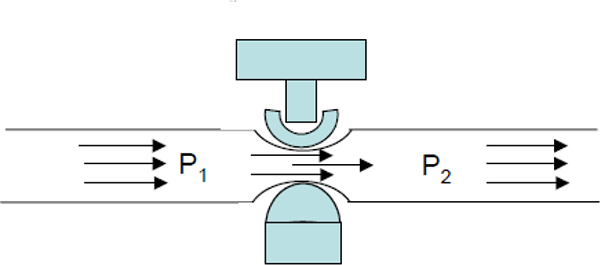
Control valve adjusts the effective area of flow in the pipe
This throttles the flow for any given pressure drop or it raises the pressure drop for any given flow.
Typical process applications can be made based on this ability to change pressure drop or flow capacity as will be seen in the next section. However, we must firstly understand how a typical control valve actually creates a pressure drop by looking at the fundamentals of flow in a pipeline and through a restricted area.
8.2.1 Turbulent and laminar flow in pipes
When a fluid is moving slowly through a pipe or if the fluid is very viscous, the individual particles of the fluid effectively travel in layers at different speeds and the particles slide over each other, creating a laminar flow pattern in a pipeline. As can be seen in Figure 8.2 the flow velocity profile is sharply curved and much higher speeds at seen at the centre of a pipeline where there is no drag effect from contact with the wall of the pipe.

Laminar flow in a pipeline has a low energy-loss rate
At higher velocities high shear forces disturb the fluid flow pattern and the fluid particles start to move in erratic paths, creating turbulent flow. This results in a much flatter flow velocity profile as can be seen in Figure 8.3. The velocity gradient is small across the centre of the pipe but is high at close proximity to the pipe wall.

Turbulent flow in a pipeline has a high energy-loss rate
The transition from laminar flow to turbulent flow can be predicted by the parameter known as the Reynolds number (Re), which is given by the equation:
Re = V. D/ν
Where: V = flow velocity, D= nominal diameter, ν = kinematic viscosity
In a straight pipe the critical values for transition form laminar to turbulent flow is approximately 3000. When the flow is turbulent, part of the flow energy in the moving fluid is used to create eddies which dissipate the energy as frictional heat and noise, leading to pressure losses in the fluid.
8.2.2 Formation of vortices
A more drastic change in velocity profile with greater energy losses arises when a fluid passes through a restrictor such as an orifice plate or a control valve opening. Downstream of a restriction there is an abrupt increase in flow area where some of the fluid will be moving relatively slowly.
Into this there flows a high velocity jet from the orifice or valve, which will cause strong vortices causing pressure losses and often creating noise if the fluid is a liquid since it is incompressible and cannot absorb the forces.
8.2.3 Flow separation
Just after the point where large increases in flow area occur, the unbalanced forces in the flowing fluid can be sufficiently high to cause the fluid close to the surface of the restricting object to lose all forward motion and even start to flow backwards. This is called the flow separation point and it causes substantial energy losses at the exit of a control valve port. It is these energy losses along with the vortices that contribute much of pressure difference created by a control valve in practice.
Figures 8.4 and 8.5 illustrate flow separation and vortices in butterfly and globe valve configurations.
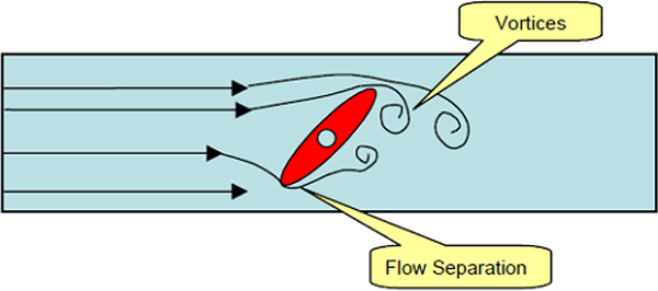
Flow separation effect in butterfly valve
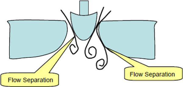
Flow separation effects in a single seated globe valve
8.2.4 Flow pulsation
One of the potential problems caused by vortex formation as described by Neles Jamesbury is that if large vortices are formed they can cause excessive pressure losses and disturb the valve capacity.
Hence special measures have to be taken in high performance valves to reduce the size of vortices. These involve flow path modifications to shape the flow paths and create “micro vortices”. Understanding fluid dynamics and separation effects contributes to control valve design in high performance applications particularly in high velocity applications when noise and vibration effects become critical.
8.2.5 Principles of valve throttling processes
The following notes are applicable to incompressible fluid flow as applicable to liquids but these can be extended to compressible flow of gases if expansion effects are taken into account. These notes are intended to provide a basic understanding of what happens inside a control valve and should serve as a foundation for understanding the valve sizing procedures we are going to study in later chapters.
A control valve modifies the fluid flow rate in a process pipeline by providing a means to change the effective cross sectional area at the valve. This in turn forces the fluid to increase its velocity as passes through the restriction. Even though it slows down again after leaving the valve, some of the energy in the fluid is dissipated through flow separation effects and frictional losses, leaving a reduced pressure in the fluid downstream of the valve.
To display the general behaviour of flow through a control valve the valve is simplified to an orifice in a pipeline as shown in Figure 8.6.
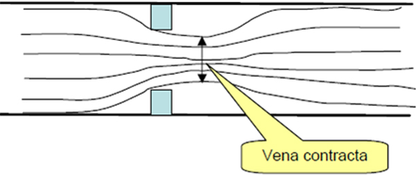
Flow through an orifice showing vena contracta point of minimum area
Figure 1.6 shows the change in the cross-section area of the actual flow when the flow goes through a control valve. In a control valve the flow is forced through the control valve orifice, or a series of orifices, by the pressure difference across the valve. The actual flow area is smallest at a point called vena contracta (Avc), the location of which is typically slightly downstream of the valve orifice, but can be extended even into the downstream piping, depending on pressure conditions across the valve, and on valve type and size.
It is important to understand how the pressure conditions change in the fluid as it passes through the restriction and the vena contracta and then how the pressure partially recovers as the fluid enters the downstream pipe area. The first point to note is that the velocity of the fluid must increase as the flow area decreases. This is given by the continuity of flow equation:

Where: V = mean velocity and A = flow area.
Subscript 1 refers to upstream conditions
Subscript 2 refer to down stream conditions
Hence we would expect to see that maximum velocity occurs at the vena contracta point. Now to consider the pressure conditions we apply Bernoulli’s equation, which demonstrates the balance between dynamic, static and hydrostatic pressure. Energy must be balanced each side of the flow restriction so that:

Where:
P = static pressure
ρ = density
Δ P = pressure loss (due to losses through the restrictor)
H = relative height
g = acceleration of gravity
The hydrostatic pressure is due to the relative height of fluid above the pipeline level (i.e. liquid head) and is generally constant for a control valve so we can simplify the equation by making H1 =H2.
The dynamic pressure component is (½ x ρ1 x V12) at the entry velocity, rising to (½ x ρ2 x V22) as the fluid speed increases through the restriction. Due to the reduction in flow area a significant increase in flow velocity has to occur to give equal amounts of flow through the valve inlet area (Ain) and vena contracta area (Avc). The energy for this velocity change is taken from the valve inlet pressure, which gives a typical pressure profile inside the valve. The velocity and the dynamic pressure fall again as the velocity decreases after the vena contracta.
The static pressure P experiences the opposite effect and falls as velocity increases and then recovers partially as velocity slows again after the vena contracta. This effect is called pressure recovery but it can be seen that there is only a partial recovery due the pressure loss component, Δ P.
The interchange of static and dynamic pressure can be seen clearly in Figure 8.7 where the pressure profile is shown as the fluid passes through the restriction and the vena contracta. The sum of the two pressures gives the total pressure energy in the system and shows the pressure loss developing as the vena contracta point is reached.
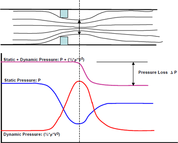
Static and dynamic pressure profiles showing pressure loss
The pressure recovery after the Vena Contracta point depends on the valve style, and is represented by valve pressure recovery factor (FL) as given in equation below. The closer the valve pressure recovery factor (FL) is to 1.0, the lower the pressure recovery.

The dynamic pressure profile corresponds to a flow velocity profile so that we can also see what happens to the fluid speed as it travels through a control valve. Figure 1.8 shows a simplified pressure and velocity profile as a fluid passes through a basic single seat control valve. It can be seen that the fluid reaches a high velocity at the vena contracta.
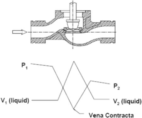
Static pressure and velocity profiles across a single seat control valve
We shall see later how the pressure profile is critical to the performance of the control valve because the static pressure determines the point at which a liquid turns to vapour. Flashing will occur if the pressure falls below the vapour pressure value and cavitation will result if condensing occurs when the pressure rises again.
Figure 8.8 therefore represents the typical velocity and pressure profiles that we can expect through a control valve. Now we need to outline the basic flow versus pressure relationship for the control valve that arises from these characteristics.
8.2.6 Pressure to flow relationships
For sizing a control valve we are interested in knowing how much flow we can get through the valve for any given opening of the valve and for any given pressure differential. Under normal low flow conditions and provided no limiting factors are involved, the flow through the control valve as derived from the Bernoulli equation is given by:

Where Q = the volumetric flow in the pipeline (= Area of pipe x mean velocity)
Δ P is the overall pressure drop across the valve and ρ is the fluid density
This relationship is simple if the liquid or gas conditions remain within their normal range without a change of state or if the velocity of the gas does not reach a limiting value. Hence for a simple liquid flow application the effective area for any control valve can be found by modelling and experiments and it is then defined as the flow capacity coefficient Cv.
Hence we can show that the flow versus square root of pressure drop relationship for any valve is given in the form shown in Figure 8.9 as a straight line with slope Cv.
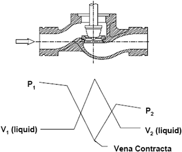
Basic flow verses pressure drop relationship for a control valve (sub-critical flow)
8.2.7 Definition of the valve coefficient Cv
The flow coefficient, Cv, or its metric equivalent, Kv, has been adopted universally as a comparative value for measuring the capacity of control valves. Cv is defined as the number of US gallons/minute at 60°F that will flow through a control valve at a specified opening when a pressure differential of 1 pound per square inch is applied.
The metric equivalent of Cv is Kv, which is defined as the amount of water that will flow in m3/hr with a 1 bar pressure drop. Converting between the two coefficients is simply based on the relationship:
Cv = 1.16 Kv
In its simplest form for a liquid the flow rate provided by any particular Cv is given by the basic sizing equation: 
Where SG is the specific gravity of the fluid referenced to water at 60°F and Q is the flow in US Gallons per minute. Hence a valve with a specified opening giving Cv =1 will pass 1 US gallon of water (at 60°F) per minute if 1 psi pressure difference exists between the upstream and downstream points each side of the valve. For the same pressure conditions if we increase the opening of the valve to create Cv =10 it will pass 10 US gallons/minute provide the pressure difference across the valve remains at 1 psi.
In metric terms: 
Where Q is in m3/hr and Δ P is in bars and SG =1 for water at 15°C.
Hence the same a valve with a specified opening giving Cv =1 will pass 0.862 m3/hr of water (at 15°C) if 1 bar pressure difference exists between the upstream and downstream points each side of the valve.
These simplified equations allow us to see the principles of valve sizing. It should be clear that if we know the pressure conditions and the SG of the fluid and we have the Cv of the valve at the chosen opening we can predict the amount of flow that will pass.
Unfortunately it is not always as simple as this because there are many factors which will modify the Cv values for the valve and there are limits to the flow velocities and pressure drops that the valve can handle before we reach limiting conditions. The most significant limitations that we need to understand at this point in the training are those associated with choked flow or critical flow as it also known. Here is brief outline of the meaning and causes of choked flow.
8.3 Cavitation
The pressure profile diagram in Figure 8.10 best illustrates how flashing and cavitation occur. As static pressure falls on the approach to the vena contracta, it may fall below the vapour pressure of the flowing liquid. As soon as this happen vapour bubbles will form in the liquid stream, with resulting expansion and instability effects.
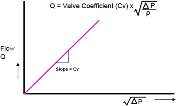
Pressure Profiles for flashing and cavitation
In the diagram the bubbles so formed are collapsing again as the pressure rises after the vena contracta and the fluids leave the valve as a liquid. This is cavitation, which can potentially damage the internals of the valve. Figure 8.11 illustrates the same effect in the flow profile through a simple valve.
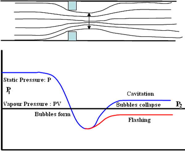
Pressure profile for cavitation in a single seated globe valve
8.4 Flashing
Flashing in the control valve also describes the formation of vapour bubbles but if the downstream pressure remains below the boiling point of the liquid, the bubbles will not condense and the flow from the valve will be partially or fully in the vapour state. Again this effect severely chokes the flow rate possible through the valve. Figure 8.12 illustrates this effect.
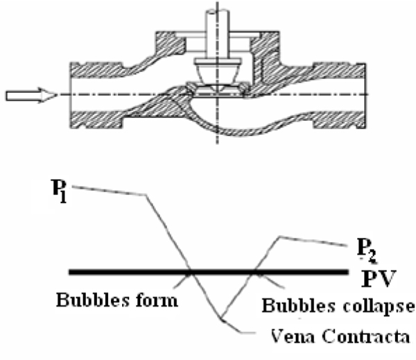
Pressure profile for flashing in a single seated globe valve
The problem in valve sizing work is determining when critical flow conditions apply, as we cannot easily see how much the static pressure will fall within a particular valve; we can only see the downstream pressure after recovery has occurred.
In this chapter we will discuss different types of Control Valves. Features of the control valves and their uses are also given.
Learning objective
- Introduction
- Globe valves
- Butterfly
- Eccentric disk
- Ball
- Rotary plug
- Diaphragm and pinch
9.1 Introduction
9.1.1 Broad classification of control valves
Figure 9.1 provides a simple classification of the most widely used types of control valves.
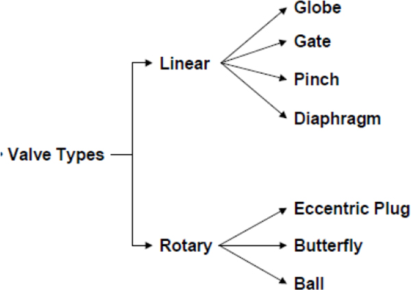
Types of control valves
The first level of grouping of valve types distinguishes between linear and rotary movement of the internal parts required to provide the variable opening required. One easy way to visualize this difference is to look at Figure 9.2 where each of the main types of valve is shown in the same pipeline.
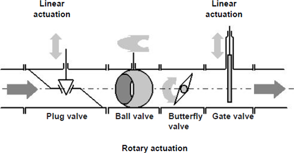
Principal types of control valve
9.2 Globe valves
The globe is the most common type of body style for sliding-stem valves. The valve body often resembles a globe divided across internally to provide two separated cavities. The valve orifice allows the fluid to pass through the body and a plug and seat are arranged to throttle and shut off the flow (Figure 9.3).
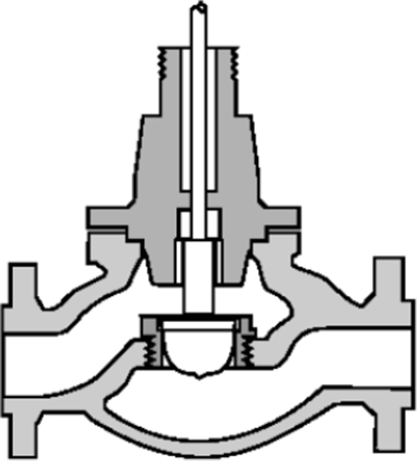
Single seated globe valve
Following are the features of globe valve:
- This valve has a linear action with a plug moving up and down.
- This valve type is very versatile, able to handle high pressures and temperatures and is made in a large variety of materials.
- Competitive on small sizes but becoming very expensive as the size increases
- Most common type of control valve used throughout world
- Well actuated with pneumatics though the forces become difficult to handle on high pressures and large sizes unless pressure balanced
- Can handle very low flow rates
- Pressure drop across valve is high compared to all other valve types
- Sizes from 12 mm to 400 mm
- Ratings to ASME 4500#
- Seat leakage to ANSI IV – optionally ANSI V + VI
- Special trims available to handle high pressure drops
The globe body differs considerably depending on the trim used. The main components of the valve trim are the plug and stem and the seat ring. The most widely used valve is the single-stage orifice and plug assembly. Multi-stage orifice elements are usually found in trim designs to reduce noise, erosion and cavitations.
Advantages
- Minimizes disassembly for maintenance
- Streamlined flow path with a minimum of parts and no irregular cavities
Disadvantages
- Leaking of the central joint due to thermal cycles or piping loads
- Valves cannot be welded in-line since the valve body is required to be split parts of a typical globe valve
Figure 9.4 shows the parts of a typical globe valve
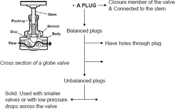
Parts of a typical globe valve
9.3 Butterfly Valves
Standard butterfly valves are dampers that are shaped from discs, which rotate in the flow path to regulate the rate of flow (Figure 9.5). The disc is quite narrow and occupies little space in the pipeline. The shaft is cantered on the axis of the pipeline and is in line with the seal. The disc pulls away from the seal upon opening. This minimizes seal wear and reduces friction. Control of the valve near the closed position can be difficult due to the breakout torque required to pull the valve out of the seat.
The flow characteristics are essentially equal percentage, but the rotation is limited to about 60 degrees as the leading edges are hidden in the shaft area as the disc is rotated further. The Fishtail is one modification of the disc that permits effective control out to 90 degrees of rotation.
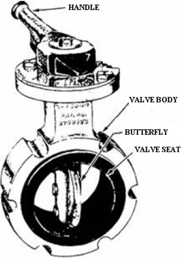
Basic butterfly valve
In its simplest form the butterfly control valve can be made with a “swivel through” disc that does not fully close of the flow, it simply provides a variable area restriction and still enables flow control to be achieved. However to provide good shutoff when closed the valve requires either soft seals around the circumference of the body or highly accurate metal seals with eccentric motion of the disc such that it is pressed tightly to seal. The soft seals are made of an elastomeric material such as rubber or Poly-tetra-fluoro-ethylene (PTFE).
Following are the features of butterfly valves
- The butterfly is a quarter turn rotary valve consisting of a disk that turns with a shaft.
- In the closed position the disk is forced into a rubber seal that deforms to create a tight seal
- The liner can be moulded to the body or can be a loose replaceable item
- The body is normally wafer style that is clamped between flanges. The liner usually serves the purpose of the line gaskets which then should not be used
- Sizes vary from 50mm to 3000mm
- Operating pressures are seldom above 1000 kPag
- These valves can be used on most applications where the pressures are low and temperatures do not exceed 100°C except when metal-seated versions are used.
- Many liner materials are available to handle different corrosive fluids
- Butterfly valves are readily actuated by pneumatics and by electrical actuators
Table 9.1 shows three typical types of butterfly valves and their characteristics. Resilient or soft-seated butterfly valves can achieve very high “bubble tight” shutoff. When fully open they present a large flow aperture and hence have a high Cv for the given line size when compare with a globe valve.
| Type of butterfly valve | Design |
|---|---|
| Resilient butterfly valve | Flexible rubber seat. Working pressure up to 1.6 Mega-Pascals (MPa)/232 pounds Per square inch (PSI) |
| High performance butterfly valve | Double eccentric in design. Working pressure up to 5.0 MPa/725 PSI |
| Tricentric butterfly valve | Metal seated design. Working pressure up to 10MPA/1450 PSI |
9.4 Eccentric disk or High performance butterfly valves
The high performance butterfly valve is a development from the conventional valve where the rotation axis of the disc is offset from both the centre line of flow and the plane of the seal (Figure 9.6). This design produces a number of advantages, including better seal performance, lower dynamic torque, and higher allowable pressure drops. The seal performance is improved because the disc cams in and out of the seat, only contacting it at closure and so wear is reduced. As the disc only approaches the seal from one side, the pressure drop across the valve can be used to provide a pressure-assisted seal. This further improves performance.
- Otherwise known as ‘high performance butterfly valves’
- Similar to the butterfly but usually supplied with a metal seat
- Good for control
- Readily actuated by pneumatics or other types
- Sizes from 50mm to 1200mm
- Pressures up to ASME 600# ( 100 bar)
- Temperatures from cryogenic to 600 degC
- Become very competitive as size Increases
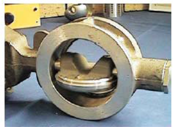
High performance butterfly valve
The modified shape and contour of the disc are used to reduce dynamic torque and drag. This also permits higher-pressure drops. As the disc is never hidden behind the shaft, good control through the 90 degrees of operation is possible with a linear characteristic. Figure 9.7 shows the butterfly disc shape.
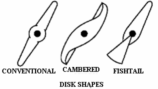
Butterfly valve disc shapes developed for improved performance range
The high performance butterfly valve is gaining greater acceptance and use due to its increased capability and the relatively high capacity to cost ratio.
Butterfly valve advantages
- Low cost and weight relative to globes as size increases
- High flow capacities
- Fire safe design
- Low stem leakage
Disadvantages
- Over sizing
- Pressure limitations
By over designing the capacity of a flow system, the result is either oversized valves, or correctly sized valves in oversized pipes. The valves in either case cause pressure drops in the flow due to the restriction. In the application of ball valves, the recovery of the pressure loss is good, but noise and cavitations then may become a problem.
9.5 Ball valves
The ball valve is one of the most common types of rotary valves available. The valve is named from the valve plug segment being a ball or sphere that rotates on an axis perpendicular to the flow stream (Figure 9.8). Fully open to fully close is performed by a 90 degree rotation of the plug segment.
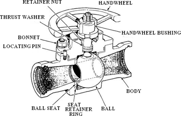
Features of the ball valve
9.5.1 The full-ball valve
The full ball valve (Figure 9.9) is shaped from a spherical segment with a cylindrical hole for the flow of fluid. Among the various configurations, the ‘floating’ ball has two seals, which provide bearing support to the ball segment. This does provide simplicity in the design; however the friction levels are higher than conventional bearing designs, which can affect control performance.
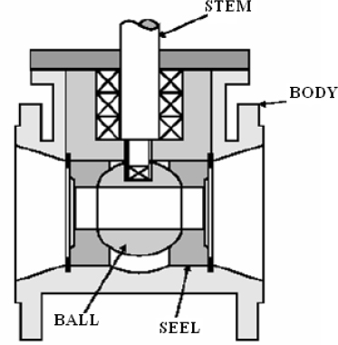
Ball Valve
Ball valves have been extensively developed for high performance on-off duties and for high range control valve duties. In shut-off duties the emphasis is on sealing designs that will provide tight shutoff and yet have minimal torque for opening.
In control valve duties many types have been developed with segmented ball trims and V-ball trims that are contoured to ensure that smooth equal percentage or linear characteristics can be achieved.
For high temperature applications metal-seated full-bore valves are available in which the ball and stem have been cast into one piece to ensure no hysteresis can occur between the stem and the ball.
Features of soft-seated ball valves:
- Simple in design and concept
- Ball with orifice through centre rotates through 90 degrees
- Line forces hold ball against downstream seat
- Seats usually made of PTFE or other elastomer
- No restriction in line when fully open so suitable for pigging
- Can be full bore (same as pipeline) or reduced bore
- Good for control
- Can be supplied in multi-port configurations
- Can be designed for high pressure when trunnion mounted
- Seat leakage to ANSI VI standard
- Can be actuated pneumatically or by other types of actuators
- Not good for slurries due to build up of material in body cavity
- Cannot handle high pressure drop applications
- Sizes from 6mm to 800mm
Features of metal-seated ball valves:
- Used for high pressure and temperature applications where PTFE cannot be used
- Metal coating can be stellite, or a ceramic coating such as tungsten carbide
- With ceramic materials sealing can be to ANSI VI or tighter if ball and seat are ground to high precision and lapped together
- This is the only valve that can be used for control applications on high temperature slurries
9.5.2 The characterized ball valve
The full-ball valve was originally designed for ON-OFF control. Although modulation control is possible, the flow characteristics can be difficult to work with. The opening between the ball and the seal can be modified to provide different flow characteristics (Figure 9.10). The V-notch is one example that produces a more gradual opening to give better range ability and throttling capability.
Most characterized ball valves are modified so that only a portion of the ball is used and these are often called segmented ball valves. The edge of the partial ball can be shaped to obtain the desired flow characteristics.
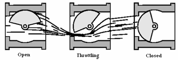
Using a segmented and characterized ball valve for modulating control
Various manufacturers promote their valves on the characteristics achieved by this design. Apart from the V-notch, other designs can be U-notch or parabolic curve. Although favourable characteristics may be achieved with the characterization of the ball, problems may occur due to the reduced strength of the partial ball. Bending is one such problem, which occurs under operating loads. Care also needs to be taken during installation as over tightening of the flange bolts can damage the seals.
Ball valve advantages
- Low cost and weight relative to globes as size increases
- High flow capacities (2 to 3 times that of globe valves)
- Tight shutoff
- Fire safe design
- Low stem leakage
- Easily fitted with quarter turn actuators
Disadvantages
- Over sizing
- High cost in large sizes compared to butterfly valves
9.6 Rotary plug valves
The plug valve (Figure 9.11) is used primarily for on-off service and some throttling services. It controls flow by means of a cylindrical or tapered plug with a hole in the centre that lines up with the flow path of the valve to permit flow. A quarter turn in either direction blocks the flow path.
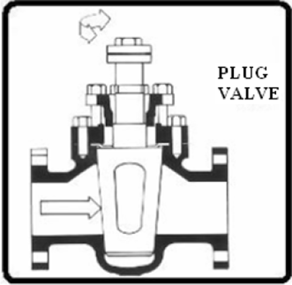
Rotary plug valve
Features of rotary plug valves:
- Similar to the ball valve but instead of a spherical ball there is a tapered plug with an orifice through the centre
- The advantage of this is that the plug can be forced further into the seat if a leak develops whereas a ball valve must be removed from the line for repair
- There is no body cavity and so this valve is more suitable for liquids that crystallize
- Most commonly used on chemical plants
- Can be fully PTFE lined
- Available in multi-port configuration for diverting or blending
- Lubricated plug valves can be used for very high pressures and for erosive applications but require high maintenance
- Non lubricated valves available from 10mm to 250mm
- Lubricated plug valves available from 50mm to 800mm
9.7 Diaphragm valves
Whilst generally used for isolation duties in water, steam and slurry applications, as well as in corrosive fluid duties the diaphragm valve can be very effectively applied to modulating control by the use of actuator and positioner system. Figure 9.12 shows the basic diaphragm valve.
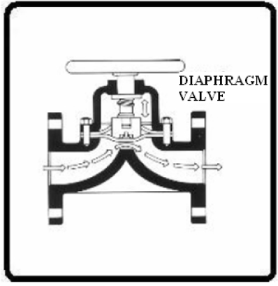
Basic diaphragm valve
Features of diaphragm valve:
- Valve design is abrasion-resistant and non-clogging
- Elastomer lined versions highly resistant to aggressive chemicals
- Suitable for throttling and on/off service in applications ranging from water treatment to chemical abrasion processes
- Operated manually, electrically, or pneumatically
- Top-entry design, allowing in-line maintenance
9.8 Pinch valves
Pinch valves (Figure 9.13) include any valve with a flexible elastomer body that can be pinched closed, cutting off flow, using a mechanism or fluid pressure. Pinch valves are full bore, linear action valves so they can be used in both an on/off manner or in a variable position or throttling service.
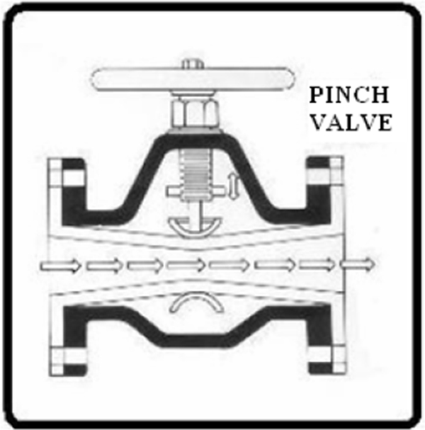
Basic pinch valve
Some typical applications for pinch valves are medical, pharmaceutical, wastewater, slurries, pulp, powder and pellets. They can effectively control the flow of both abrasives and corrosives, as there is no contact between metal parts and the transport media. The merits of the pinch valve for control duties are similar to those for the diaphragm valve.
Pinch valves may be closed either by manual means, or fluid actuation. Electromechanical closure is effected by actuating a solenoid, which then lowers a bar or gate onto the sleeve, cutting off the flow. With fluid actuated pinch valves, the pinching action is accomplished by air or hydraulic pressure placed directly on the elastomer sleeve. The valve body acts as a built-in actuator, eliminating costly hydraulic, pneumatic, or electric operators.
Pinch valves are used widely in medical, pharmaceutical and other sanitary applications. They contain a number of design advantages allowing for cleanliness, excellent drainage, and ease of cleaning. Most varieties are constructed so that the compression pressure is from the top only allowing the valve to drain thoroughly in all positions except upside down. Additionally, many have a straight-through design that allows for a high rate of flow with minimal turbulence. Both of these features call for low air consumption, allowing the system to stay relatively closed, reducing the introduction of airborne contaminants. Optional sterility features include end flange configurations that connect flush with the transport tubing; and in situations where the tubing does not connect flush, seals in both the valve and fittings to eliminate particle entrapment, and facilitate in-line cleaning. Other advantages, not specifically related to sterile operation, include low maintenance, low weight (due to the largely plastic body), and suitability for use in systems requiring explosion-proof line closure.
While the design of pinch valves provides extensive advantages for use in sterile lines, and in situations where product purity is a high priority; these same design features create some disadvantages. Due to their elastomer bodies, pinch valves are not viable in situations where the transport media is of a high temperature. They are also contraindicated for services that require high-pressure flow, and for use with gases.
This chapter will provide an over view of PLCs. The importance of PLCs and the advantages of using a PLC system will be discussed.
Learning objectives
- Introduction to PLCs
- Alternative control systems- where do PLCs fit in
- Why PLCs have become so widely accepted
10.1 Introduction to the PLC
In the past, processes were controlled manually, which was a very tedious job. During the early years of control, man constructed hardware relay wiring to control the same process. However, relays could not meet all the needs of modern times, and a faster solution was required. Simply, when a change of control logic was required, the entire hardware wiring needed to be changed. This was time consuming as well as tiresome.
After a lot of toil, man finally designed the PLC. He overcame all the constraints and attained flexibility to carry out the necessary modifications.
“PLC” means “Programmable Logic Controller”. The word “Programmable” differentiates it from the conventional hard-wired relay logic. It can be easily programmed or changed as per the application’s requirement. The PLC also surpassed the hazard of changing the wiring.
The PLC as a unit consists of a processor to execute the control action on the field data provided by input and output modules.
In a programming device, the PLC control logic is first developed and then transferred to the PLC.
10.2 Alternative control systems- where do PLCs fit in?
PLCs can do the following:
- It can perform relay-switching tasks
- It can conduct counting, calculation and comparison of analogue process values
- It offers flexibility to modify the control logic, whenever required, in the shortest time
- It responds to the changes in process parameters within fraction of seconds.
- It improves the overall control system reliability
- It is cost effective for controlling complex systems
- Trouble-shooting becomes simpler and faster
- An operator can easily interact with the process with the help of the HMI (Human-Machine Interface) computer
10.3 Why PLCs have become so widely accepted
PLCS are widely accepted due to the below advantages:
- Flexible
- Faster response time
- Less and simpler wiring
- Solid-state-no moving parts
- Modular design- easy to repair and expand
- Handles much more complicated systems
- Sophisticated instruction sets available
- Allows for diagnostics “easy to troubleshoot”
- Less expensive
Eliminates much of the hard wiring that was associated with conventional relay control circuits. Figure 10.1 shows a model diagram of a of PLC.
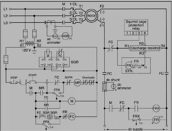
Model diagram of PLC
The program takes the place of much of the external wiring that would be required for control of a process.
Increased Reliability
Once a program has been written and tested it can be downloaded to other PLCs.
Since all the logic is contained in the PLC’S memory, there is no chance of making a logic wiring error. Figure 10.2 illustrates the increased reliability.
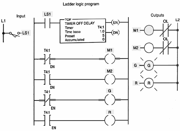
Illustration of increased reliability
More flexibility
Original equipment manufacturers (OEMs) can provide system updates for a process by simply sending out a new program.
It is easier to create and change a program in a PLC than to wire and rewire a circuit. End users can modify the program in the field. . Figure 10.3 illustrates the flexibility.
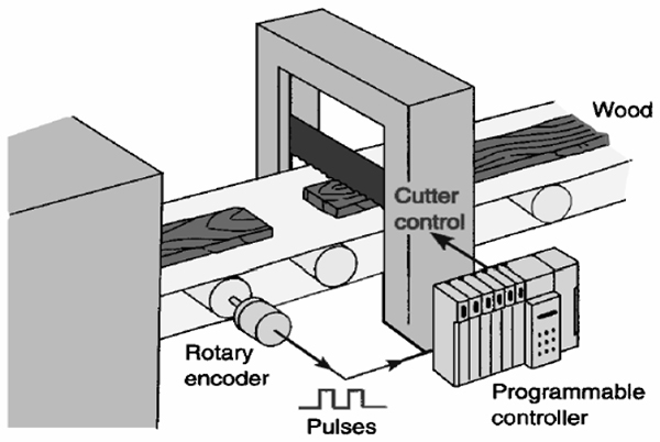
Illustration of more flexibility
Lower costs
Originally PLCs were designed to replace relay control logic. The cost saving using PLCs have been so significant that relay control is becoming obsolete, except for power applications. . Figure 10.4 shows the decreased cost.
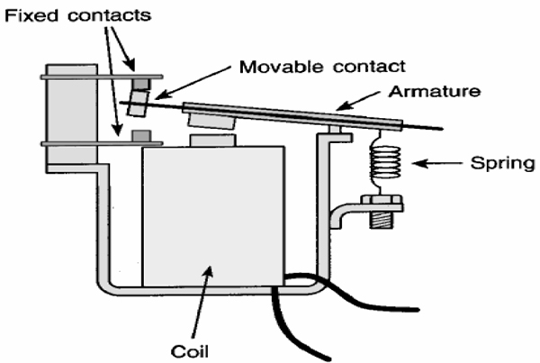
Illustration of lower cost
Generally, if an application requires more than about 6 control relays, it will usually be less expensive to install a PLC.
Communication capability
A PLC can communicate with other controllers or computer equipment. Figure 10.5 illustrates the communication capability.
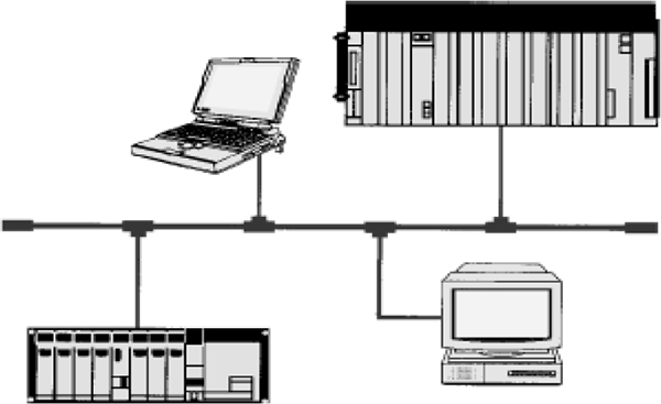
Illustration of communication capability
They can be networked to perform such function as:
- Supervisory control
- Data gathering
- Monitoring devices
- Process parameters
- Downloading and uploading of program
Faster response time
PLCs operate in real-time which means that an event taking place in the field will result in an operation or output taking place. . Figure 10.6 illustrates the fast response.
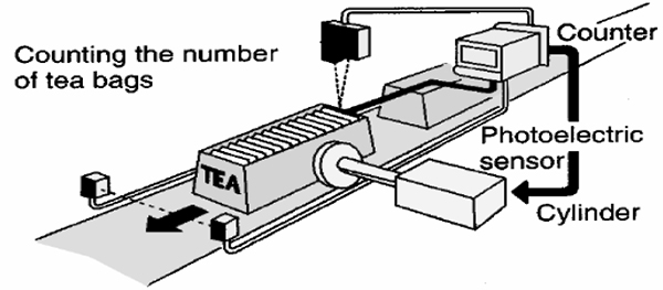
Illustration of faster response time
Machines that process thousands of items per second and objects that spend only a fraction of a second in front of a sensor require the PLCs quick response capability.
Easier to Troubleshoot
PLCs have resident diagnostic and override functions allowing users to easily trace and correct software and hardware problems. Figure 10.7 illustrates the troubleshooting.
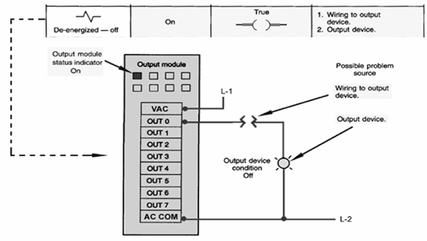
Illustration of troubleshooting
The control programs can be watched in real-time as it executes to find and fix problems.
Learning objectives
- Block diagram of typical PLC
- PLC processor module-memory organization
- Input/output section-module types
- Power supplies
11.1 Block diagram of typical PLC
Figure 11.1 shows the basic block diagram of a common PLC system.
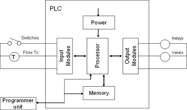
Block diagram of a PLC
As shown in the above figure, you will find the heart of the “PLC” in the centre, i.e., the Processor or CPU (Central Processing Unit)
- The CPU regulates PLC program, data storage, and data exchange with I//O modules
“I/O Modules” are the second important and basic components of any PLC system
- Input and output modules are the media for data exchange between field devices and CPU. It tells CPU6 the exact status of field devices and also acts as a tool to control them
The programming device is the third significant component
- A programming device is a computer loaded with programming software, which allows a user to create, transfer and make changes in the PLC software
Memory is the fourth notable component
- Memory provides the storage media for PLC program as well as different data
11.2 PLC processor Module – Memory organization
11.2.1 Memory systems
The memory system is an integral and very important part of any PLC system. There are two broad sections of PLC memory:
- Internal memory
- External memory
‘Internal memory’ is the memory within the PLC, i.e. the user accessible memory (RAM). It is an integral part of each PLC.
‘External memory’ is memory outside of the PLC, i.e. generally the EPROM or EEPROM. It is an optional part of any PLC, and dependant on the vendor.
The functions of user accessible memory and it’s the various types will now be discussed in detail.
Internal or user accessible memory (RAM)
Internal or user accessible RAM has following functions:
- Storing the user PLC program
- Storing the status of inputs and outputs
- Storing timer, counter and register values
Figure 11.2 describes this section of memory.

Sections of PLC RAM memory
As shown in the Fig 11.2, user accessible memory is used for storing the ‘User PLC program,’ which occupies its major portion. It is also used for storing the status of inputs and outputs, storing timer, counter and register values.
Based on these functions, PLC memory is broadly divided in two categories:
- Program memory
- Storage memory
Program memory
This is portion of memory used for storing the user PLC program. This program is actually stored in memory, by means of machine code format.
Programming is usually done in ladder, statement list or any PLC language. Following this, the program is downloaded to the PLC. As part of the download process the program is converted into machine code and stored in program memory.
The sequence for machine code instructions is very similar to the sequence of user programs just discussed.
The program memory occupies the largest portion of total memory usage. For example, a system with 16K memory words may have program memory ranging from 4K to 12K words, depending on the complexity of the program.
The complexity or size of the process decides the size/space of memory required in the PLC’s CPU. This is a major factor in the selection of a CPU, as once the system is commissioned, it is very important that there be enough space still left, for future program additions.
Storage memory
This portion of memory stores the important information related to program execution such as the present status of the inputs and outputs, timer, counter, register values, etc.
It does not occupy much space, but dictates the maximum number of timers, counters and registers that one can use in the program.
Storage memory can be described as storing the following information:
- Process input and output image. That is the online status of real world analogue and digital inputs, as well as outputs.
- Preset and accumulated values of timers and counters.
- Values of temporary storage bits and registers.
- Storing system related data such as hardware configuration of the system, CPU related diagnostic information, etc.
Please note that to prevent the loss of data in case of a power failure, it is very important to have a battery backup as all of the above-mentioned information is stored in RAM.
Normally, all PLCs have a battery for memory backup. Along with it, as seen earlier, there is a ‘battery healthy’ indication on the CPU as well.
External memory (EEPROM)
This is the optional memory that can be plugged externally into the slot provided on the PLC CPU.
It may generally be either an EPROM or EEPROM type of memory. As the EEPROM offers more flexibility (by means of easier program changes), it has become the more popular of the two.
Functions of external memory:
- Storing the user PLC program permanently.
- Avoids program loss in case of a power failure.
- Allows the user to transfer the altered PLC program using standard programming devices.
A copy of the PLC program can be stored on the external memory. If this is done, one need not worry about power failures any more. Some PLCs offer an alternate option. For example, the program in the external memory may be copied automatically into the internal memory after a power failure. Such a feature is provided, to safeguard the internal PLC program.
However, if the good battery backup is supplied for the RAM memory, then this external memory is not required.
11.3 Input/output section – Module types
11.3.1 Basics of Analogue I/O systems
Analogue means a continuous signal, i.e. one that does not just have two states, as would be found with a typical discrete signal. An analogue signal has a continuous value, the range of which depends on the analogue module type.
When reference is made to a continuous signal, it means the field device is sensing the process parameter variations, as they occur, on a continuous basis. This varying signal is given as an input to the analogue module or taken as an output from the analogue module.
Although these modules are found in reduced ratios in typical PLC systems (when compared to Digital I/O), they remain one of the most important modules in any PLC system.
Whenever there is continuous control of any process parameter, analogue input and analogue output modules are definite requirement. The analogue input module collects the process parameter feedback, and passes it to the PLC.
During program execution, the control (or manipulated) variable value is transferred from the PLC to the field through analogue output modules to execute control action.
Similar to DI/DO modules, analogue modules are exchange data with the CPU, through a back. To interact with a continuous analogue signal, AI/AO modules have a special circuit (called an ADC or DAC) inside, that converts the analogue signal to/from a digital equivalent.
11.3.2 Types of analogue input modules
Similar to DI/DO modules, analogue modules can be plugged in different PLC racks. Depending on their locations, they can be classified as:
Master or CPU rack modules
This refers to the rack in which a PLC CPU is plugged. This rack may or may not provide slots for accepting analogue I/O modules, depending on vendor and configuration. If the system is small, it will generally provide slots for analogue I/O modules. For larger systems, no free slots (for plugging analogue I/O modules) may be provided in the Master Rack module.
Local rack modules
These racks are often located just beside or below the master rack. They provide slots for the plugging in of analogue I/O modules. Data is exchanged with the CPU, through a local rack communication processor.
Remote rack modules
Remote racks are located at a remote location, along with various I/O modules. They exchange data with the CPU, through a remote communication processor.
Depending on whether standard analogue signals used, the following types of analogue modules may be utilised:
- 4 to 20mA DC signal
- 0 to 20mA DC signal
- 0 to +10 volts DC signal
- -10V to +10V DC signal
- 0 to 5 V DC signal
- RTD/thermocouple type
Many PLC vendors supply a combination-type analogue module, which may support a combination of the above signal types. They can be configured for any of the more common signal types, mentioned above.
Some of the various different types of analogue input connections, to the PLC, will now be discussed individually.
11.3.3 Types of analogue output modules
Analogue output modules can be used to supply either current or voltage values to loads. Depending on the analogue signals required, the following analogue modules are available:
- 4 to 20mA DC signal
- 0 to 20mA DC signal
- 0 to +10 V DC signal
- -10 to +10 V DC signal
- 0 to 5 V DC signal
Some PLC vendors may even provide an analogue module that can be configured for any of the available signal types, as just mentioned above.
Connections of various types of analogue signals will now be show connected to the module.
11.3.4 Basics of discrete I/O systems
Digital signals coming and going to discrete field devices have only two states—‘On’ or ‘Off’. This ‘On’ or ‘Off’ signal is given to a PLC via the digital input modules. Program execution takes place based on the status of the input signals. At the end of execution, appropriate ‘On’ or ‘Off’ output commands are given to discrete field devices through digital output modules.
Thus, this interaction between discrete field devices and the PLC takes place through DI and DO modules. The DI/DO modules exchange signals with the field through hard wiring. However, signal exchange with the PLC takes place through the back plane connectors’ data bus.
DI/DO modules are plugged into the rack, which is the enclosure used for accommodating all the I/O modules. Depending on where the modules are plugged, the rack is broadly divided as
Master or CPU rack: The rack into which the PLC CPU is plugged. This rack may [or may not] provide slots for plugging the I/O modules, depending on the vendor and the configuration. If the system is small, it may generally provide slots for I/O modules. There are no free slots for plugging I/O modules, for the large systems.
Local rack 1: This rack lies just beside the master rack. It provides slots for plugging I/O modules. Data is exchanged with the CPU through a local rack communication processor. In most cases, you will find that the master rack works as a local rack.
Local rack 2: This rack is located at a remote location along with I/O modules. It exchanges data with the CPU through a remote communication processor.
11.3.5 Types of discrete input modules
Different digital input modules are available to access the different types of discrete field devices. They will now be discussed individually.
Discrete DC input module
These modules are widely used for their low voltage level signals and compatibility with several discrete field devices.
Figure 11.3 shows the termination diagram, as well as a section of the internal circuit for most common types of 24VDC digital input (sink-type) modules.
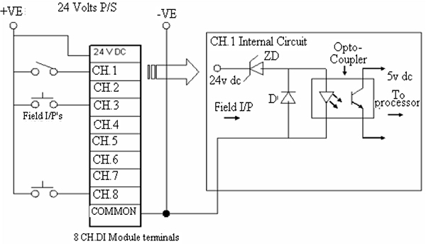
Digital DC input module
As shown in Fig. 11.3, discrete field devices are connected to an eight-channel DI module (24V DC type). The module is supplied with 24VDC, and a common terminal provided.
The internal circuit of one channel is shown in the same figure. The field voltage input is compared with a preset threshold, for the detection of ‘Logic 1’ and ‘Logic 0’ state.
Generally, if the input voltage is above 12V, it is sensed as ‘Logic 1’ signal. Similarly, if the input voltage is below 6V, it is sensed as ‘Logic 0’ signal. This input signal then goes through an opto-isolator and an optically isolated signal (5V DC), and is given to the processor’s internal circuit.
The opto-isolator is provided for isolating the field circuit from the internal circuit. The opto-coupler provides noise immunity, as well as isolation between the field and the processor. This also acts as a safety feature against voltage spikes that may occur in the field. A typical digital input module will have an LED for each channel, to show the logic status of the input signal. By either glowing or not, the LED provides an indication of the input’s status. In some instances, one may also find a fuse protection along with a fuse blown LED indicator.
Discrete AC input module
These are normally used for interfacing discrete AC field devices with the PLC. One will generally find these modules are used for interfacing MCC signals with the PLC.
Figure 11.4 shows the termination diagram, as well the section of internal circuit, for a 230VDC digital input module.
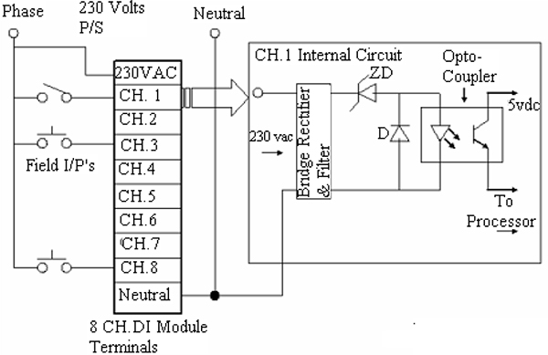
Discrete AC input module
Other than the power section, everything else within a Discrete AC Input module remains the same for a channel internal circuit.
The power section includes a bridge rectifier and a noise filter unit. A bridge rectifier converts the 230VDC signal into DC voltage. This voltage signal then passes through a filter circuit that filters out any noise in the incoming signal. Following this, the DC level signal passes through a threshold detection circuit, which detects the ‘logic state’ of the signal. After passing through the opto-isolator circuit, the logic ‘1’ or ‘0’ signal is passed to the internal circuit.
Fuse protection is provided for the power section. An LED indicator is used to indicate the state of the fuse, i.e. whether it is healthy or not. An LED’s are also provided, for indicating the logical status of all incoming signals.
Isolated DC/AC input module
These modules are similar to the previous modules, except that each and every input has a separate common.
11.3.6 Types of discrete output modules
Discrete output modules are, typically some of the most commonly used modules in PLC applications.
Various discrete field devices (such as solenoids, auxiliary contactors, on/off valves, lights, alarms, motor starters, etc.) are operated using these ‘discrete output modules’ of the PLC. Since many discrete field devices have various voltage requirements for operation, different types of discrete output modules are available. Generally module output voltage levels may be indicated as follows:
- 12 to 30VDC
- 110V AC/DC
- 230V AC/DC
11.4 Power supplies
11.4.1 PLC power supply
A DC power supply is required, by the PLC, for low-level voltage used by the CPU, as well as for the I/O and communication modules. More often than not, a separate power supply module mostly supplies power. This is located beside the CPU unit or the external power supply, depending on the PLC vendor.
The voltage required depends on the type of chips used within the system. If TTL ICs are used, a 5V DC power supply will be required. If a CMOS type of IC is utilized, then the power supply will be in the range of 3V to 18V.
This is the internal power supply for the PLC unit and is often referred to as the internal power supply.
Power is also required for operating field devices and output loads, in order that they may operate. A separate external power supply is provided for this purpose. It is often referred to as the field interrogation power supply.
The latter is kept separate from the control power supply; so that any power supply problems in the field are not echoed within the PLC.
It is good practice to isolate all power supplies and keep their commons separate. It is also necessary to take care of the ground connection properly, as it is very important for a PLC system to have safe and reliable power supplies.
11.4.2 PLC panel power supply
The PLC panel power supply is used for following purposes:
- Supply power to PLC rack consisting modules
- Supply power to load power supplies (field interrogation power supply)
- Supply power to lighting and other utilities inside panel
Generally, separate Miniature Circuit Breakers (MCBs) are provided for individual units so that, in the event of a breakdown of individual equipment, only that equipment gets isolated from the main power supply.
Ensure that the AC power source for the PLC system is isolated (through a constant voltage transformer or isolation transformer if possible) from any sources of electrical noise.
For PLC installations near sources of electrical interference, an isolation transformer is a recommended approach. Note that the output devices being controlled should draw power from the original source of the voltage unless the secondary of the isolation transformer (which is supplying the computers) has been specifically rated for these additional devices.
Where the AC power source has variations, a Constant Voltage Transformer (CVT) can stabilize the voltage for short periods of time, thus minimizing shutdowns. It is worth noting here, that CV transformers are very sensitive to variations in mains frequency and will not operate successfully with unstable mains frequency supplies (see Figure 11.5).
For both the CVT and the isolation transformer the operating frequency and the operating voltage should be carefully specified (e.g. 240VAC + 10%- 15% or 50Hz ± 2%).
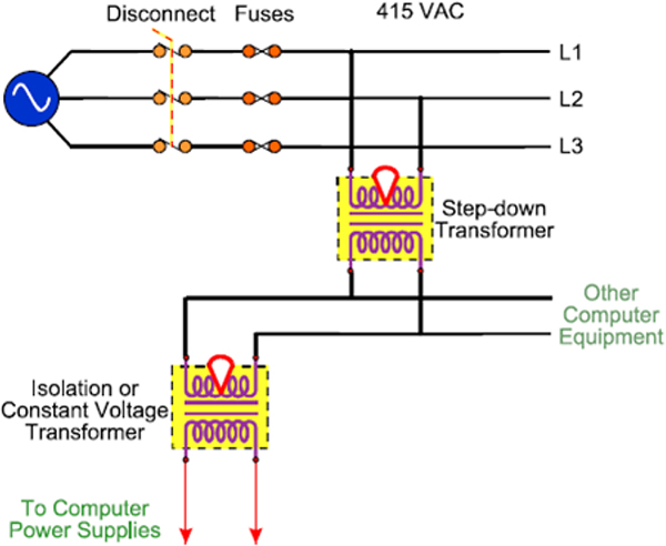
An isolation transformer
It is important to size transformers correctly:
- If the transformer is too small, it will clip the peaks off the sine wave (due to saturation) resulting in a lower RMS value of the voltage. The power supply could sense this as a low voltage and shutdown. The transformer may also overheat and burn out
- Excessively large transformers do not provide as much isolation as a correctly sized transformer, due to higher capacitive coupling
Where power supply is variable in frequency, or unreliable, or where the PLC requires high power supply security, the UPS (uninterruptible power supply) is often selected. Its size in KVA rating is decided as per the system load.
An online UPS converts raw AC power into DC voltage by first using a rectification unit and then coverts the same DC voltage into AC using an inverter unit and feeds the same to the load. In the event of power failure of raw AC, it starts taking DC voltage through batteries and converts into AC, and feeds the same to load.
Useful techniques to reduce the electromagnetic interference and switching transients are given in Figure 11.6
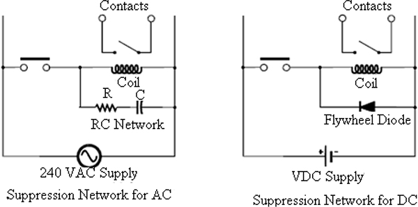
Techniques for reducing electromagnetic interference and surges
In this chapter we will discuss methods of representing logic, basics related to Ladder logic, basic rules for programming and simple PLC programs.
Learning objectives
- Methods of representing Logic
- Ladder Logic basics
- The basic rules for programming
- Simple PLC programs
12.1 Methods of representing logic
12.1.1 Basic logic instructions
These instructions are basically representative of the ON/Off status of the inputs and also for changing the output status. They are also referred as ‘Bit’ type instructions and can be written as follows:
- XIC (Examine if Close)
- XIO (Examine if Open)
- OTE (Turn a bit to ‘True’/’False’)
- OTL (Latch a bit to ‘True’ state)
- OTU (Latch a bit to ‘False’ state)
- OSR (One Shot Rising)
XIC (Examine if Close): This instruction is used for checking the bit status (logic 1) of a digital input or an internal memory bit.
In order for this to happen, the ‘XIC’ instruction is referenced to the input or internal bit address. If the bit is ‘On’ when the instruction is executed, the result of logic operation is ‘True’, as a ‘Normally Open’ contact will change to a ‘Closed’ state.
On the contrary, if the addressed bit indicates that it is in the ‘Off’ state, then the result of the logic operation is ‘False’. Figure 12.1 shows the XIC symbol.

Symbol of XIC
As shown in the symbol, the bit can either be a storage bit or a physical input (e.g., I: 1.0/3). An output coil or a memory bit always follows this instruction.
XIO (Examine if Open): This instruction is used for checking the bit status (logic 0) of a digital input or an internal memory bit.
Once again, for this to happen, the ‘XIC’ instruction is referenced to the input or internal bit address. If the bit is ‘Off’ when the instruction is executed, then the result of logic operation is ‘True’. Think in terms of the ‘Normally Closed’ contact of a STOP button. It will remain ‘Closed’ if the switch is not pressed. Alternately, if the bit addressed is ‘On’, then the result of logic operation is ‘False’. Figure 12.2 shows the XIO symbol.
Symbol of XIO
The bit can be a storage bit or a physical Input (e.g., I:1.0/3), as shown in figure12.2. An output coil or memory bit always follows this instruction.
OTE (Turn a bit to ‘True’/’False’): Coils or outputs represent relays that are energized when power flows to them. When a coil is energized, it causes the corresponding output to turn on, by changing the state to logic ‘1’.
The output instruction turns a bit (storage bit or physical output) status or output coil to logical ‘0’ (Off) condition or to logical ’1’ (On) depending on the result of logic operation of ladder rung. If rung is ‘True,’ the coil will turn ‘On’. If not, it will be in the ‘Off’ state.
‘XIC’ and ‘XIO’ instructions are found in front of OTE instructions, in order to check the status of the bits. Figure 12.3 shows the OTE symbol.
Symbol of OTE
If the OTE instruction is used after the ‘XIC’ input, a logical input ‘1’ will set the rung true and cause the output to turn ‘On’. If used after the ‘XIC’, logical input ‘0’will set the rung false and cause the output to turn ‘Off’.
As shown in the figure, a bit can either be a storage bit or a physical output (e.g., O:0.3/5). This instruction is always at the right hand side of the ladder rung.
OTL (Latch a bit to ‘True’ state): This instruction is similar to the ‘OTE’ instruction except that it ‘Latches’ the output to ‘On’ state. This instruction latches a bit (storage bit or physical output) to logical ‘1’ (On) condition when the rung goes ‘True’.
It will remain ‘On’ until the same bit is turned ‘Off’ using the ‘OTU’ (i.e. latch a bit to ‘False’ state or unlatch, as sometimes referred to) instruction. Figure 12.4 shows the OTL symbol.
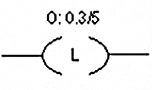
Symbol of OTL
As shown in the above figure, a bit can either be a storage bit or a physical output (e.g., O:0.3/5). This instruction is always on the right hand side of the ladder rung.
OTU (Latch a bit to ‘False’ state): This instruction is similar to the ‘OTL’ instruction except that it ‘Un-Latches’ the output from an ‘On’ to an ‘Off’ state. Both these instructions are complimentary to each other.
This instruction latches a bit (storage bit or physical output) to logical ‘0’ (Off) condition. It will remain ‘Off’ unless the same bit is turned ‘On’ using the ‘OTL’ (Latch a bit to ‘True’ state) instruction. Figure 12.5 shows the OTU symbol.
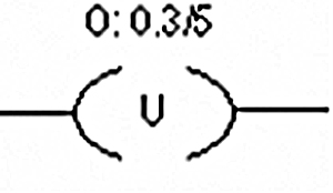
Symbol of OTU
As shown in the figure, a bit can either be a storage bit or a physical output (e.g., O: 0.3/5). This instruction is found at the right hand side of the ladder rung.
OSR (One Shot Rising): When the rung goes from a ‘False’ to a ‘True’ state, the OSR (One Shot Relay) instruction will turn ‘On’ for one scan, and thereafter, it will be turn ‘Off’ for all following scans.
It is used specifically for the detection of a change of state of a rung from ‘False’ to ‘True’ and turns a bit (storage bit or physical output) status to a logical ’1’ (On) condition for one scan, only. Hence, the output bit status will change only for this one scan. Figure 12.6 shows the OSR symbol.
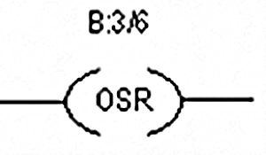
Symbol of OSR
OSR instructions require a bit address (binary/integer). Bear in mind that the same bit address cannot be used elsewhere in the program.
12.2 Ladder Logic basics
The ladder-logic approach to programming is popular because of its perceived similarity to standard electrical circuits. Two vertical lines supplying the power are drawn at each of the sides of the diagram with the lines of logic drawn in horizontal lines.
The example below shows the ‘real world’ circuit with PLC acting as the control device and the internal ladder-logic within the PLC. Figure 12.7 shows the ladder logic.
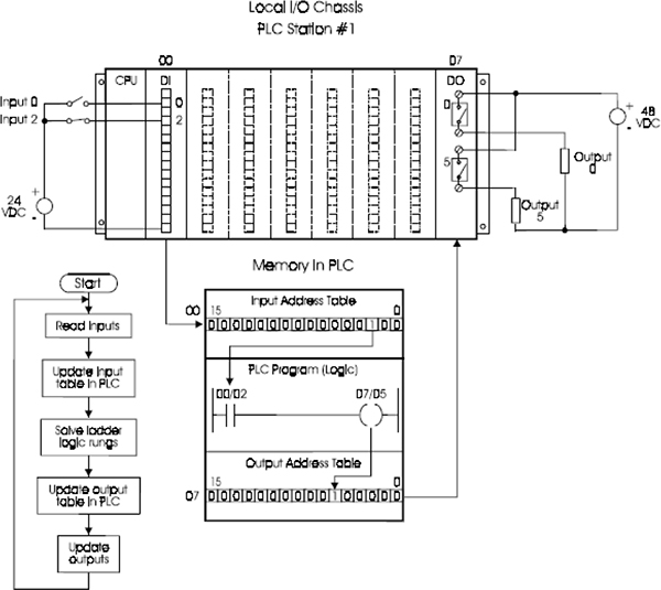
The concept of PLC ladder-logic
12.2.1 Basic rules of ladder-logic
The basic rules of ladder-logic can be stated to be:
- The vertical lines indicate the power supply for the control system (12 V DC to 240 V AC). The ‘power flow’ is visualized to move from left to right.
- Read the ladder diagram from left to right and top to bottom (as in the normal Western convention of reading a book).
- Electrical devices are normally indicated in their normal de-energized condition. This can sometimes be confusing and special care needs to be taken to ensure consistency.
- The contacts associated with coils, timers, counters and other instructions have the same numbering convention as their control device.
- Devices that indicate a start operation for a particular item are normally wired in parallel (so that any of them can start or switch the particular item on). See Figure 12.8 for an example of this.
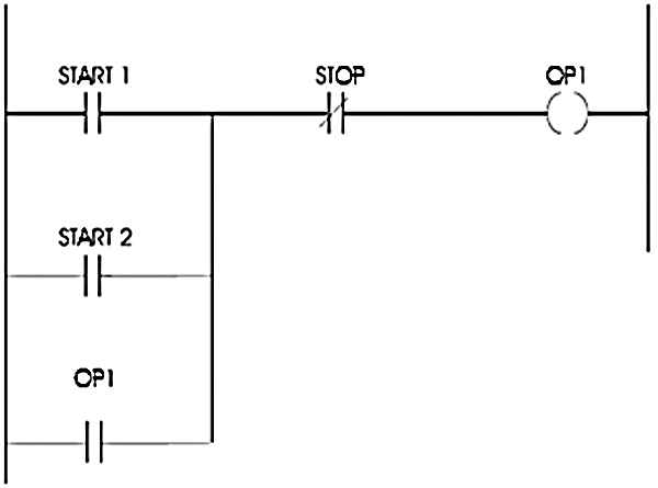
Ladder-logic start operation (& logic diagram)
- Devices that indicate a stop operation for a particular item are normally wired in series (so that any of them can stop or switch the particular items off). See Figure 12.9 for an example of this.
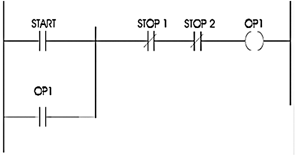
Ladder-logic stops operation (& logic diagram)
- Latching operations are used, where a momentary start input signal latches the start signal into the on condition, so that when the start input goes into the OFF condition, the start signal remains energized ON. The latching operation is also referred to as holding or maintaining a sealing contact. See the previous two diagrams for examples of latching.
- Interactive logic: Ladder-logic rungs that appear later in the program often interact with the earlier ladder-logic rungs. This useful feed back mechanism
12.2.2 The different ladder-logic instructions
Ladder-logic instruction can be typically broken up into the following different Categories:
- Standard relay logic type
- Timer and counters
- Arithmetic
- Logical
- Move
- Comparison
- File manipulation
- Sequencer instructions
- Specialized analogue (PID)
- Communication instructions
- Diagnostic
- Miscellaneous (sub routines etc)
12.3 The basic rules for programming
PLC programming steps
Once the programmer has the tools for PLC programming he can proceed to the actual function of programming, itself.
To develop a PLC program for any process or system, simply follow the steps given below:
- Understanding the process and define the control philosophy
- Ensure the preparation of a control strategy
- Create a flowchart
- Implement the flowchart, using selected programming languages
These steps are applicable to all PLCs with the IEC 1131-3 programming standard, and independent of the process application. They can be used for developing a PLC program for any type of PLC and any process.
12.3.1 Understanding process and defining control philosophy
Before developing a PLC program for a particular process, it is very important to first understand the process. Right from program development to commissioning, you will need the knowledge of the process you are dealing with.
After doing that, develop a ‘Control Philosophy,’ which defines what needs to be done for achieving process control under process limits and serves as a platform for control program.
Since each process has different aspects of engineering, such as operation, electrical, instrumentation, mechanical, chemical, etc., it is important to formulate the ‘Control Philosophy’ jointly with people who know and understand these various aspects.
Depending on the inputs from the process, a final control philosophy is prepared, and this serves as a reference for a programmer. Sometimes, this is also referred to as the ‘Control Task’ for a process control.
12.3.2 Preparation of control strategy (algorithm)
Once the ‘Control Philosophy’ is formalized, the programmer can start applying his mind at to how to accomplish the tasks mentioned, in the most optimized manner.
Firstly, the ‘Control Philosophy’ task is divided into different groups, by studying the sequence of events that take place / happen in a process.
Next, the individual group tasks are further sub-divided into parts and a solution (output results) is sought for all the sections. This is referred to as the process of building an ‘Algorithm’ or control strategy.
After building the control strategy for the first time, alternative approaches (to obtain similar output results), should also be considered.
It is important that time be set aside to think and rethink the solution algorithm over and over, until it is as polished as possible. The basic purpose of emphasizing this is to reduce the programming time in the long run.
This will also reduce the debugging time and ensure a smooth and accelerated start-up.
12.3.3 Creating a flowchart
With each step, the programmer moves closer and closer towards the PLC program development. The objective of following these steps is to approach the task at hand in a systematic manner so as to minimize any mistakes.
A PLC programmer should always be aware of a fact that, even though the PLC does have tremendous functional capability; it still is only capable of doing what it has been told to do. Therefore, the programmer should always be aware of what he is telling the PLC to do.
‘Flowcharts’ are developed to represent the programming steps in a pictorial manner, for ease of use and understanding. They indicate the flow and sequence of events in a particular section, along with their relationship to each other in the most simplified manner.
Flowcharts may be prepared per individual process, and are then referred to as ‘Sub-routines’. Various sub-routines can be called in a main flowchart, as per the process sequence.
Flowchart symbols have specific meanings, and these are there to simplify their interpretation.
Figure 12.10 shows a typical process flowchart of a ‘Tank Level control’ system. The task has been divided into different steps, as per the sequence of events, and the interrelation of these steps has been clearly shown.
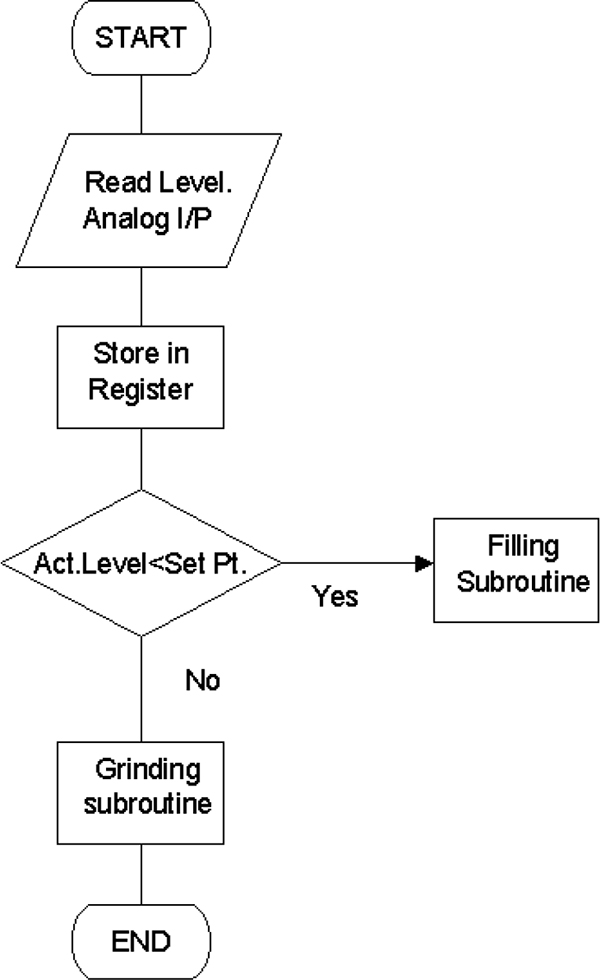
Program flowcharting
Once the control objective is fulfilled, the program will be terminated at the ‘END’. The ‘Decision making’ block decides on the path of execution of logic. In the main flowchart, it will be found that sub-routines are called to execute a sub-task. In the above example, the ‘Grinding sub-routine’ will be executed only if the (decision-making block) result is ‘No’. In all other instance, the program will continue executing the ‘Filling sub-routine’.
In this manner, different program control flowcharts are prepared and interlinked to the main flowchart.
In this chapter we will discuss the fundamentals of SCADA. A comparison between SCADA, DCS, PLC and smart instruments is given. Installation of a typical SCADA system is explained and the important terms used in the SCADA system are highlighted.
Learning objectives
- Fundamentals
- Comparison of SCADA, DCS,PLC and smart instruments
- Typical SCADA installations
- Definition of terms
13.1 Fundamentals
In modern manufacturing and industrial processes, mining industries, public and private utilities, leisure and security industries telemetry is often needed to connect equipment and systems separated by large distances. This can range from a few meters to thousands of kilometres. Telemetry is used to send commands, programs and receives monitoring information from these remote locations.
SCADA refers to the combination of telemetry and data acquisition. SCADA encompasses the collecting of the information, transferring it back to the central site, carrying out any necessary analysis and control and then displaying that information on a number of operator screens or displays. The required control actions are then conveyed back to the process.
In the early days of data acquisition, relay logic was used to control production and plant systems. With the advent of the CPU and other electronic devices, manufacturers incorporated digital electronics into relay logic equipment. The PLC or programmable logic controller is still one of the most widely used control systems in industry. As need to monitor and control more devices in the plant grew, the PLCs were distributed and the systems became more intelligent and smaller in size. PLCs and DCS (distributed control systems) are used as shown below figure 13.1.
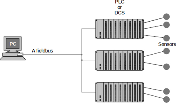
PC to PLC or DCS with a field bus and sensor
The advantages of the PLC / DCS / SCADA system are:
- The computer can record and store a very large amount of data
- The data can be displayed in any way the user requires
- Thousands of sensors over a wide area can be connected to the system
- The operator can incorporate real data simulations into the system
- Many types of data can be collected from the RTUs
- The data can be viewed from anywhere, not just on site
The disadvantages are:
- The system is more complicated than the sensor to panel type
- Different operating skills are required, such as system analysts and programmer
- With thousands of sensors there is still a lot of wire to deal with
- The operator can see only as far as the PLC
As the requirement for smaller and smarter systems grew, sensors were designed with the intelligence of PLCs and DCSs. These devices are known as IEDs (intelligent electronic devices). The IEDs are connected on a field bus, such as Profibus, Device net or Foundation Field bus to the PC. They include enough intelligence to acquire data, communicate to other devices, and hold their part of the overall program. Each of these super smart sensors can have more than one sensor on-board. Typically, an IED could combine an analogue input sensor, analogue output, PID control, and communication system and program memory in one device. Figure 13.2 shows a connection of PC to IED through a field bus.
PC to IED using a field bus
The advantages of the PC to IED field bus system are:
- Minimal wiring is needed
- The operator can see down to the sensor level
- The data received from the device can include information such as serial numbers, model numbers, when it was installed and by whom
- All devices are plug and play, so installation and replacement is easy
- Smaller devices means less physical space for the data acquisition system
The disadvantages of a PC to IED system are:
- More sophisticated system requires better trained employees
- Sensor prices are higher (but this is offset somewhat by the lack of PLCs)
- The IEDs rely more on the communication system
13.2 Comparison of SCADA, DCS, PLC and smart instruments
13.2.1 SCADA system
A SCADA (or supervisory control and data acquisition) system means a system consisting of a number of remote terminal units (or RTUs) collecting field data connected back to a master station via a communications system. The master station displays the acquired data and also allows the operator to perform remote control tasks.
The accurate and timely data (normally real-time) allows for optimization of the operation of the plant and process. A further benefit is more efficient, reliable and most importantly, safer operations. This all results in a lower cost of operation compared to earlier non-automated systems.
There is a fair degree of confusion between the definition of SCADA systems and process control system. SCADA has the connotation of remote or distant operation. The inevitable question is how far ‘remote’ is – typically this means over a distance such that the distance between the controlling location and the controlled location is such that direct-wire control is impractical (i.e. a communication link is a critical component of the system).
A successful SCADA installation depends on utilizing proven and reliable technology, with adequate and comprehensive training of all personnel in the operation of the system. There is a history of unsuccessful SCADA systems – contributing factors to these systems includes inadequate integration of the various components of the system, unnecessary complexity in the system, unreliable hardware and unproven software. Today hardware reliability is less of a problem, but the increasing software complexity is producing new challenges. It should be noted in passing that many operators judge a SCADA system not only by the smooth performance of the RTUs, communication links and the master station (all falling under the umbrella of SCADA system) but also the field devices (both transducers and control devices). The field devices however fall outside the scope of SCADA in this manual and will not be discussed further. A diagram of a typical SCADA system is given opposite. Figure 13.3 shows the diagram of a typical SCADA system.
Diagram of a typical SCADA system
On a more complex SCADA system there are essentially five levels or hierarchies:
- Field level instrumentation and control devices
- Marshalling terminals and RTUs
- Communications system
- The master station(s)
- The commercial data processing department computer system
The RTU provides an interface to the field analogue and digital signals situated at each remote site.
The communications system provides the pathway for communications between the master station and the remote sites. This communication system can be radio, telephone line, microwave and possibly even satellite. Specific protocols and error detection philosophies are used for efficient and optimum transfer of data.
The master station (and sub-masters) gather data from the various RTUs and generally provide an operator interface for display of information and control of the remote sites. In large telemetry systems, sub-master sites gather information from remote sites and act as a relay back to the control master station.
SCADA technology has existed since the early sixties and there are now two other competing approaches possible – distributed control system (DCS) and programmable logic controller (PLC). In addition there has been a growing trend to use smart instruments as a key component in all these systems. Of course, in the real world, the designer will mix and match the four approaches to produce an effective system matching his/her application. Figure 13.4 shows a SCADA system.
SCADA system
13.2.2 Distributed control system (DCS)
In a DCS, the data acquisition and control functions are performed by a number of distributed microprocessor-based units situated near to the devices being controlled or the instrument from which data is being gathered. DCS systems have evolved into systems providing very sophisticated analogue (e.g. loop) control capability. A closely integrated set of operator interfaces (or man machine interfaces) is provided to allow for easy system configurations and operator control. The data highway is normally capable of fairly high speeds (typically 1 Mbps up to 10 Mbps). Figure 13.5 shows a DCS system.
Distributed control system (DCS)
13.2.3 Programmable logic controller (PLC)
Since the late 1970s, PLCs have replaced hardwired relays with a combination of ladder– logic software and solid state electronic input and output modules. They are often used in the implementation of a SCADA RTU as they offer a standard hardware solution, which is very economically priced. Sample PLC system is shown in figure 13.6.
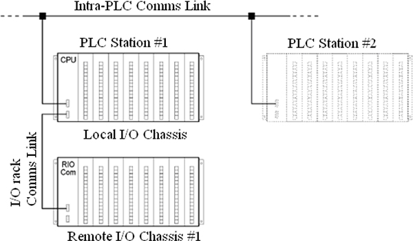
Programmable logic controller (PLC) system
Another device that should be mentioned for completeness is the smart instrument which both PLCs and DCS systems can interface to.
13.2.4 Smart instrument
Although this term is sometimes misused, it typically means an intelligent (microprocessor based) digital measuring sensor (such as a flow meter) with digital data communications provided to some diagnostic panel or computer based system. Figure 13.7 shows an example of a smart instrument.
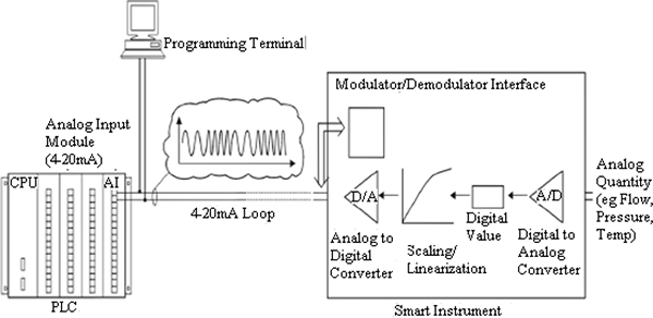
Typical example of a smart instrument
13.2.5 Considerations and benefits of SCADA system
Typical considerations when putting a SCADA system together are:
- Overall control requirements
- Sequence logic
- Analogue loop control
- Ratio and number of analogue to digital points
- Speed of control and data acquisition
- Master/operator control stations
- Type of displays required
- Historical archiving requirements
- System consideration
- Reliability/availability
- Speed of communications/update time/system scan rates
- System redundancy
- Expansion capability
- Application software and modelling
Obviously, a SCADA system’s initial cost has to be justified. A few typical reasons for implementing a SCADA system are:
- Improved operation of the plant or process resulting in savings due to optimization of the system
- Increased productivity of the personnel
- Improved safety of the system due to better information and improved control
- Protection of the plant equipment
- Safeguarding the environment from a failure of the system
- Improved energy savings due to optimization of the plant
- Improved and quicker receipt of data so that clients can be invoiced more quickly and accurately
- Government regulations for safety and metering of gas (for royalties & tax etc)
13.3 Typical SCADA installations
13.3.1 Guidelines for electrical installation
Equipotential bonding
Between separate sections of an installation, potential differences can develop if:
- Cable shields are connected at both ends and are grounded at different parts of the system
- Different AC supplies, for example, can cause potential differences. Installing equipotential bonding conductors to ensure functioning of the electronic components can reduce these differences
The following points must be observed for equi-potential bonding:
- The lower the impedance of the equipotential bonding conductor, the greater the effectiveness of equipotential bonding
- Where shielded signal lines are laid between the relevant sections of the system and connected at both ends to the ground/protective conductor, the impedance of the additional equipotential bonding conductor must not exceed 10 percent of the shield impedance
The cross-section of the equipotential bonding conductor must be rated for the maximum circulating current. The following cross-sections of copper have proved to be satisfactory in practice:
- 16 mm sq. of copper for equipotential bonding conductors of up to 200m in length
- 25 mm sq. of copper for equipotential bonding conductors of more than 200m in length.
- Use copper or zinc-plated steel for equipotential bonding conductors. They must be given a large-area connection to the ground/protective conductor and protect it from corrosion.
- The equipotential bonding conductor should be laid so that the smallest possible areas are enclosed between the equipotential bonding conductor and signal lines.
- Create a standard reference potential
- Ground all electrical apparatus if possible.
- Use specific grounding measures. Grounding of the control system is a protective and functional measure.
- System parts and cabinets with central controllers and expansion units should be connected to the ground/protective conductor system in star configuration. This serves to avoid the creation of ground loops.
- In case of potential differences between system parts and cabinets, install equipotential bonding conductors of sufficient rating.
Suppressing interference
Measures for suppressing interference voltages are often applied only when the control system is already operational and proper reception of a useful signal is impaired. The reason for such interference is usually inadequate reference potentials caused by mistakes in the equipment assembly.
The following sections describe:
- Basic rules for grounding the inactive metal parts
- Examples of cabinet assembly for EMC
Basic rules for assembling and grounding inactive metal parts
Ensure a wide-area chassis grounding of the inactive metal parts when mounting the equipment. Properly implemented grounding creates a uniform reference potential for the control system, and reduces the effects of picked-up interference. Chassis grounding is understood to mean the electrical connection of all inactive parts. The entirety of all interconnected inactive parts is the chassis ground. Inactive parts are conductive parts that are electrically isolated from active parts by basic insulation, and can only develop a voltage in the event of a fault.
The chassis ground must not develop a dangerous touch voltage, even in the event of a fault. The ground must therefore be connected to the protective ground conductor.
To prevent ground loops, locally separated ground elements such as cabinets, structural and machine parts, must always be connected to the protective ground system in star configuration. Ensure the following when chassis grounding:
- Connect the inactive metal parts with the same degree of care as the active parts.
- Ensure low-impedance metal-to-metal connections, e.g., with large-area, good quality contact.
- When you are incorporating painted or anodized metal parts in the grounding, these insulating protective layers must be penetrated. Use special contact washers or remove the insulating layer.
- Protect the connection points from corrosion, e.g., with grease.
- Movable grounded parts such as cabinet doors must be connected via flexible grounding strips. The grounding strips should be short and have a large surface because the surface is decisive in providing a path to ground for high-frequency interference.
These are the important aspects of a PLC panel ‘Electrical design and construction’, which one should be familiar with. They play a very important role in the smooth working of a PLC system.
13.4 Definition of terms
HMI: HMI stands for Human Machine Interface. The HMI is also referred as supervisory system or operator system
Interlocks: These are devices (with output contact/s) related to the process, integrally mounted on or near a piece of equipment. Process interlocks may be by passed under controlled conditions without endangering human and/or compromising operating safety of machines, whilst safety interlocks cannot be bypassed.
Sequence: A sequence is a part of a software program configured to start-up, control and/or shut down associated plant equipment in a pre-determined and logical manner.
Devices (software based): These are software modules encapsulating the functionality of equipment control and diagnostics. Example motors, valves, sequences, analogues etc
DCS (Distributed Control System): A distributed control system is a grouping of dedicated electronic devices suited for visualization, interlocking, sequence control, drive control and feedback control on processes with high level of instrumentation.
PLC (Programmable logic Controller): A Programmable logic controller is a software programmable electronic device. It is suited for interlocking, sequence control, drive control, and feed back control. The functionality of these devices has been increased to include fuzzy logic control, feed forward and multivariable control.
SCADA: SCADA means Supervisory Control And Data Acquisition. By means of key-board actions and screen displays the SCADA system allows the operators to control associated process. Also referred to as an MMI (Man Machine Interface), or HMI (Human Machine Interface)
In this chapter we will discuss about the remote terminal unit (RTU) structure, analogue and digital input/output modules and master site structure.
Learning objectives
- Remote Terminal Unit (RTU) structure
- Analogue and Digital input/output modules
- Master site structure
14.1 Remote Terminal Unit (RTU) structure
An RTU (sometimes referred to as a Remote Telemetry Unit) as its title implies is a standalone data acquisition and control unit, generally microprocessor based, which monitors and controls equipment at some remote location from the central station. Its primary task is to control and acquire data from process equipment at the remote location and to transfer this data back to a central station. It generally also has the facility for having its configuration and control programs dynamically downloaded from some central station. There is also a facility to be configured locally by some RTU programming unit. Although traditionally the RTU communicates back to some central station, it is also possible to communicate on a peer-to-peer basis with other RTUs. The RTU can also act as a relay station (sometimes referred to as a store and forward station) to another RTU which may not be accessible from the central station.
Small sized RTUs generally have less than 10 to 20 analogue and digital signals; medium sized RTUs have 100 digital and 30 to 40 analogue inputs. RTUs having a capacity greater than this can be classified as large. A typical RTU configuration is shown in Figure 14.1.
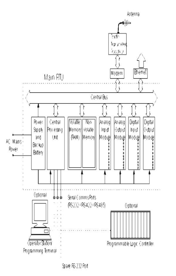
Typical RTU hardware structure
A short discussion follows on the individual hardware components. Typical RTU hardware modules include:
- Control processor and associated memory
- Analogue inputs
- Analogue outputs
- Counter inputs
- Digital inputs
- Digital outputs
- Communication interface(s)
- Power supply
- RTU rack and enclosure
14.2 Analogue and digital Input /Output modules
14.2.1 Analogue input modules
There are five main components making up an analogue input module. They are:
- The input multiplexer
- The input signal amplifier
- The sample and hold circuit
- The A/D converter
- The bus interface and board timing system
A block diagram of a typical analogue input module is shown below in Figure 14.2.
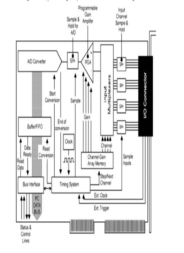
Block diagram of a typical analogue input module
Each of the individual components will be considered in the following sections.
Multiplexers
A multiplexer is a device that samples several (usually 16) analogue inputs in turn and switches each to the output in sequence. The output generally goes to an A/D converter, eliminating the need for a converter on each input channel. This can result in considerable savings.
Amplifier
Where low-level voltages need to be digitized, they must be amplified to match the input range of the board’s A/D converter. If a low-level signal is fed directly into a board without amplification, a loss of precision will be the result. Some boards provide on-board amplification (or gain), while those with a PGA make it possible to select – from software – different gains for different channels, for a series of conversions.
Sample-and-hold circuit
Most A/D converters require a fixed time during which the input signal remains constant (the aperture time) in order to perform an A/D conversion. This is a requirement of the conversion algorithm used by the A/D converter. If the input were to change during this time, the A/D would return an inaccurate reading. Therefore, a sample-and-hold device is used on the input to the A/D converter. It samples the output signal from the multiplexer or gain amplifier very quickly and holds it constant for the A/Ds aperture time.
The standard design approach is to place a simple sample-and-hold chip between multiplexer and A/D converter.
A/D converters
The A/D converter is the heart of the module. Its function is to measure an input analogue voltage and to output a digital code corresponding to the input voltage.
There are two main types of A/D converters used:
- Integrating A/Ds
- Successive Approximation A/Ds
Integrating (or Dual Slope) A/Ds—these are used for very low frequency applications (a few hundred samples per second maximum) and may have very high accuracy and precision (e.g. 22 bit). They are found in thermocouple and RTD modules. Other advantages include very low cost, noise and mains pickup tend to be reduced by the integrating and dual slope nature of the A/D converter.
The A/D procedure essentially requires a capacitor to be charged with the input signal for a fixed time, and then uses a counter to calculate how long it takes for the capacitor to discharge. This length of time is proportional to the input voltage.
Successive Approximation A/Ds—Successive approximation A/Ds allow much higher sampling rates (up to a few hundred thousand samples per second with 12 bits is possible) while still being reasonable in cost.
The conversion algorithm is similar to that of a binary search, where the A/D starts by comparing the input with a voltage (generated by an internal D/A converter), corresponding to half of the full scale range. If the input is in the lower half the first digit is zero and the A/D repeats this comparison using the lower half of the input range. If the voltage had been in the upper half, the first digit would have been 1 and the next comparison in the upper half of the input range. This dividing of the remaining fraction of the input range in half and comparing to the input voltage continues until the specified numbers of bits of accuracy have been obtained.
The bus interface provides the mechanism for transferring the data from the board and into the host PCs memory, and for sending any configuration information (for example, gain/channel information) or other commands to the board. The interface can be either 8-, 16- or 32-bit.
14.2.2 Analogue input configurations
It is important to take proper care when connecting external transducers or similar devices (the signal source); otherwise the introduction of errors and inaccuracies into a data acquisition system is virtually guaranteed.
Connection methods
There are two methods of connecting signal sources to the data acquisition board: Single-ended and differential; they are shown below. In general, differential inputs should be used for maximum immunity. Single-ended inputs should only be used where it is impossible to use either of the other two methods.
Single-ended Inputs—Boards which accept single-ended inputs have a single input wire for each signal, the source’s HI side. All the LO sides of the sources are commoned and connected to the analogue ground AGND pin. This input type suffers from loss of common mode rejection and is very sensitive to noise. It is not recommended for long leads (longer than ½ m) or for high gains (greater than 5x). The advantage of this method is that it allows the maximum number of inputs, is simple to connect (only one common or ground lead necessary) and it allows for simpler A/D front end circuitry. We can see from Figure 14.3 that because the amplifier LO (Negative) terminal is connected to AGND, what is amplified is the difference between Esn + VCM and AGND, and this introduces the common mode offset as and error into the readings. Some boards do not have an amplifier, and the multiplexer output is fed straight to the A/D. Single-ended inputs must be used with these types of boards. Figure 14.3 shows eight single ended inputs.
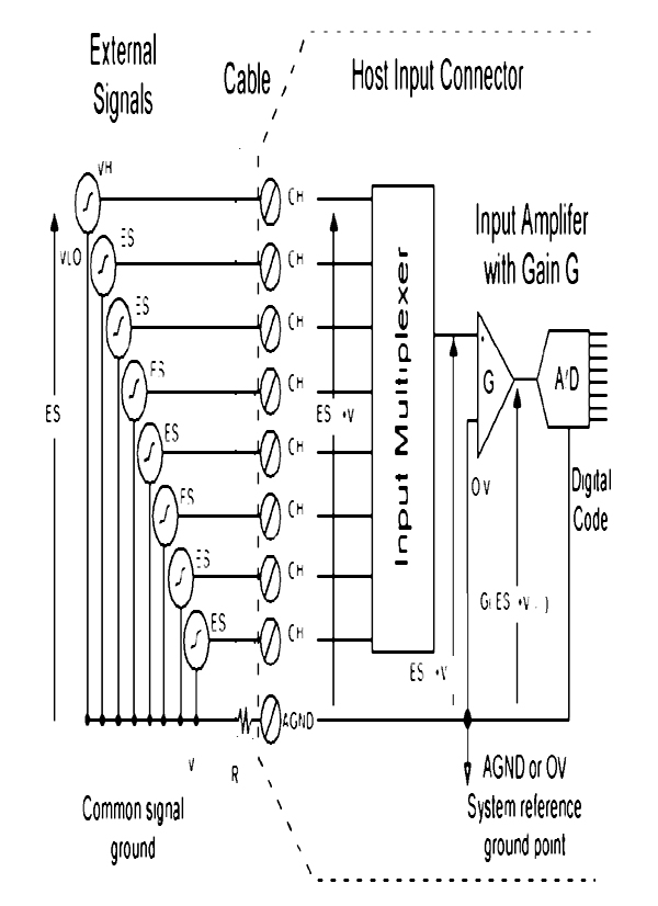
Eight single-ended inputs
Differential Inputs—True differential inputs provide the maximum noise immunity. This method must also be used where the signal sources have different ground points and cannot be connected together. Referring to Figure 14.4, we see that each channel’s individual common mode voltage is fed to the Amplifier negative terminal; the individual VCMn voltages are thus subtracted on each reading.
Note that two input multiplexers are needed, and for the same number of input terminals as single-ended and pseudo-differential inputs, only half the number of input channels are available in differential mode. Also, bias resistors may be required to reference each input channel to ground. This depends on the board’s specifications (the manual will explain the exact requirements) but it normally consists of one large resistor connected between each signal’s LO side and AGND (at the signal end of the cable) and sometimes it requires another resistor of the same value between the HI side and AGND.
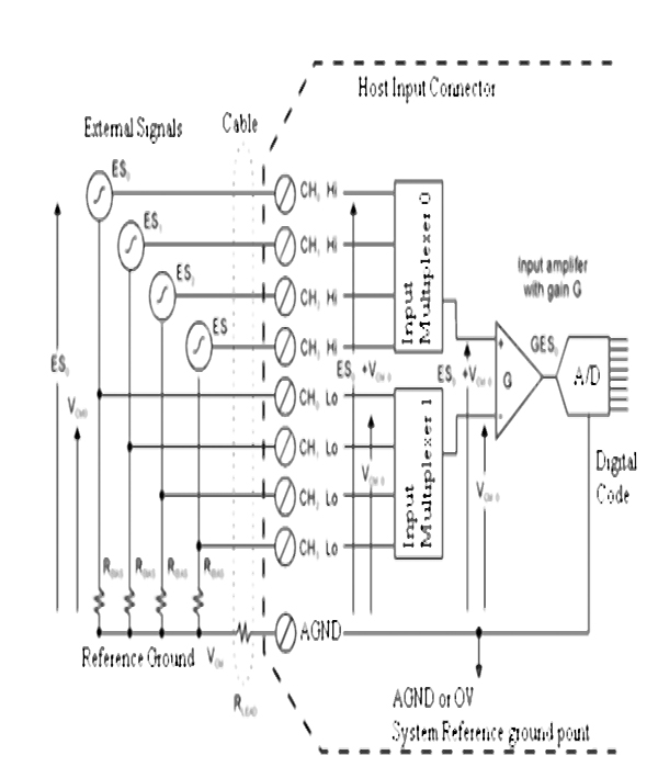
Four differential inputs
Note that VCM and VCMn voltages may be made up of a DC part and possibly a time-varying AC part. This AC part is called noise, but we can see that using differential inputs, the noise part will also tend to be cancelled out (rejected) because it is present on both inputs of the input amplifier.
14.2.3 Typical analogue input modules
These have various numbers of inputs. Typically there are:
- 8 or 16 analogue inputs
- Resolution of 8 or 12 bits
- Range of 4-20 mA (other possibilities are 0-20 mA/±10 Volts/0-10 Volts)
- Input resistance typically 240 kΩ to 1 MΩ
- Conversion rates typically 10 microseconds to 30 milliseconds
- Inputs are preferably differential rather than single ended for better noise immunity
For reasons of cost and minimization of data transferred over a radio link, a common configuration is eight single ended 8 bit points reading 0-10 Volts with a conversion rate of 30 milliseconds per analogue point.
An important but often neglected issue with analogue input boards is the need for sampling of a signal at the correct frequency. The Nyquist criterion states that a signal must be sampled at a minimum of two times its highest component frequency. Hence the analogue to digital system must be capable of sampling at a sufficiently high rate to be well outside the maximum frequency of the input signal. Otherwise filtering must be employed to reduce the input frequency components to an acceptable level. This issue is often neglected due to the increased cost of installing filtering with erroneous results in the measured values. It should be realized the software filtering is NOT a substitute for an inadequate hardware filtering or sampling rate. This may smooth the signal but it does not reproduce the analogue signal faithfully in a digital format.
14.2.4 Analogue outputs
Typical analogue output module
Typically the analogue output module has the following features:
- 8 analogue outputs
- Resolution of 8 or 12 bits
- Conversion rate from 10µ seconds to 30 milliseconds
- Outputs ranging from 4 – 20 mA/± 10 Volts/0 to 10 Volts
Care has to be taken here on ensuring the load resistance is not lower than specified (typically 50 kΩ) or the voltage drop will be excessive.
Analogue output module designs generally prefer to provide voltage outputs rather than current output (unless power is provided externally), as this places lower power requirements on the backplane.
14.2.5 Digital inputs
These are used to indicate such items as status and alarm signals. Status signals from a valve could comprise two limit switches with and contact closed indicating valve – open status and the other contact closed indicating valve – closed status. When both open and closed status contacts are closed, this could indicate the valve is in transit. (There would be a problem if both status switches indicate open conditions). A high level switch indicates an alarm condition.
It is important with alarm logic that the RTU should be able to distinguish the first alarm that occurred from the subsequent spurious alarms that occur.
Most digital input boards provide groups of 8, 16 or 32 inputs per board. Multiple boards may need to be installed to cope with numerous digital points (where the count of a given board is exceeded).
The standard normally open or normally closed converter may be used for alarm. Generally normally closed alarm digital inputs are used where the circuit is to indicate an alarm condition.
The input power supply must be appropriately rated for the particular convention used – normally open or normally closed. For the normally open convention, it is possible to derate the digital input power supply.
Optical isolation is a good idea to cope with surges induced in the field wiring. A typical circuit and its operation is indicated in Figure 14.5.
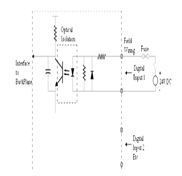
Digital input circuit with flow chart of operation
The two main approaches of setting the input module up as a sink or source module are as indicated Figure 14.6 below.
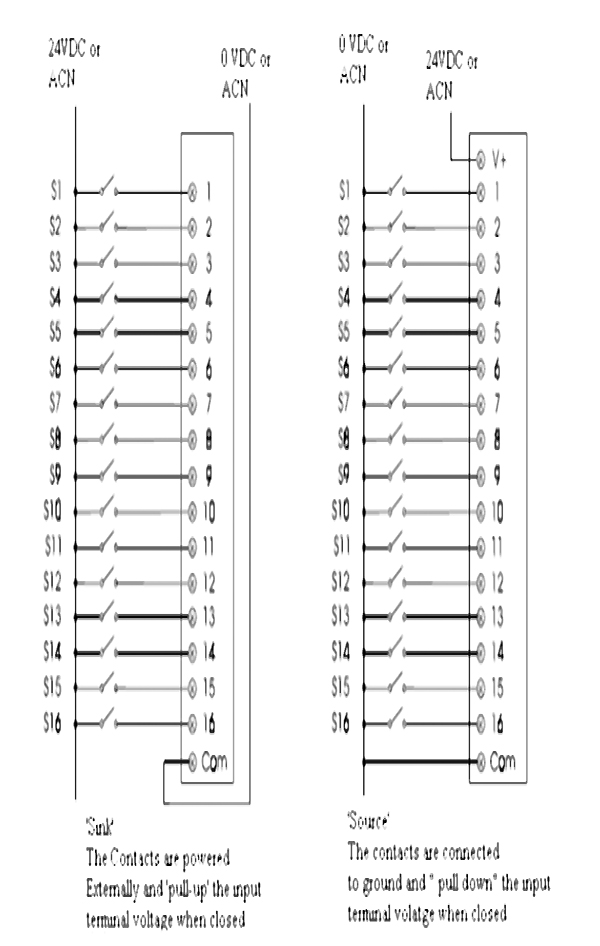
Configuring the input module as a sink or source
Typical digital input module
Typically the following would be expected of a digital input module:
- 16 digital inputs per module
- Associated LED indicator for each input to indicate current states
- Digital input voltages vary from 110/240 VAC and 12/24/48 VDC
- Optical isolation provided for each digital input
14.2.6 Counter or accumulator digital inputs
There are many applications where a pulse input module is required – for example from a metering panel. This can be a contact closure signal or if the pulse frequency is high enough – solid state relay signals.
Pulse input signals are normally “dry contacts” (i.e. the power is provided from the RTU power supply rather than the actual pulse source).
Figure 14.7 below gives the diagram of the counter digital input system. Optical isolation is useful to minimize the effect of externally generated noise. The size of the accumulator is important when considering the number of pulses that will be counted, before transferring the data to another memory location. For example, a 12-bit register has the capacity for 4096 counts. 16 bits gives 65536 pulses which could represent 48 minutes at 20 000 barrels/hour, for example. If these limits are ignored, the classical problem of the accumulator cycling through zero when full could occur.
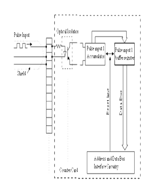
Pulse input module
Two approaches are possible:
- The accumulator contents can be transferred to RAM memory at regular intervals where the old and current values difference can be stored in a register
- The second approach is where a detailed and accurate accounting needs to be made of liquids flowing into and out of a specific area. A freeze accumulator command is broadcast instantaneously to all appropriate RTUs. The pulse accumulator will then freeze the values at this time and transfer to a memory location, and resets the accumulator so that counting can be resumed again
Typical counter specifications
The typical specifications here are:
- 4 counter inputs
- Four 16 bit counters (65536 counts per counter input)
- Count frequency up to 20 kHz range
Duty cycle preferably 50% (ratio of mark to space) for the upper count frequency limits. Note that the duty rating is important as the counter input needs a finite time to switch on (and then off). If the on pulse is too short, it may be missed although the count frequency is within the specified limits.
A Schmitt trigger gives the preferred input conditioning although a resistor capacitor combination across the counter input can be a cheap way to spread the pulses out.
14.2.7 Digital output module
A digital output module drives an output voltage at each of the appropriate output channels with three approaches possible:
- Transistor switching
- Triac switching
- Reed relay switching
- TTL voltage outputs
The TRIAC is commonly used for AC switching. A varistor is often connected across the output of the TRIAC to reduce the damaging effect of electrical transients. Three practical issues should also be observed:
- A TRIAC output switching device does not completely switch on and off but has low and high resistance values. Hence although the TRIAC is switched off it still has some leakage current at the output
- Surge currents should be of short duration (half a cycle). Any longer will damage the module
- The manufacturer’s continuous current rating should be adhered to. This often refers to individual channels and to the number of channels. There are situations where all the output channels of the module can be used at full rated current capacity. This can exceed the maximum allowable power dissipation for the whole module
Typical digital output modules
Typically the digital output module has the following features:
- 8 digital outputs
- 240 VAC/24 VDC (0.5 Amp to 2.0 Amp) outputs
- Associated LED indicator for each output to indicate current status
- Optical isolation or dry relay contact for each output (see Figure 14.8)
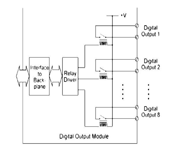
Digital output module
“Dry” relay contacts (i.e. no voltage applied to the contacts by the output module) are often provided. These could be reed relay outputs for example. Ensure that the current rating is not exceeded for these devices (especially the inductive current). Although each digital output could be rated at 2 Amps; the module as a whole cannot supply 16 Amps (8 by 2 Amps each) and there is normally a maximum current rating for the module of typically 60% of the number of outputs multiplied by the maximum current per output.
If this total current is exceeded there will be overheating of the module and eventual failure.
Note also the difference sinking and sourcing of an I/O module. If a module sinks a specified current, it means that it draws this current from an external source. If a module sources a specific current it drives this current as an output (see Figure 14.9).
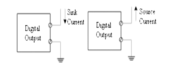
Source and sink of current
When connecting to inductive loads it is essential to put a flywheel diode across the relay for DC systems and a capacitor/resistor combination for AC systems as indicated in Figure 14.10. This dissipates the energy in the magnetic field of the inductor when the devices are switched off. And minimizes the consequent voltage spikes produced across the switching element. Such voltage spikes could otherwise exceed the reverse voltage ratings of silicon switching devices, such as transistors, thyristors or TRIACs, causing their destruction or shorten the life of relay contacts.
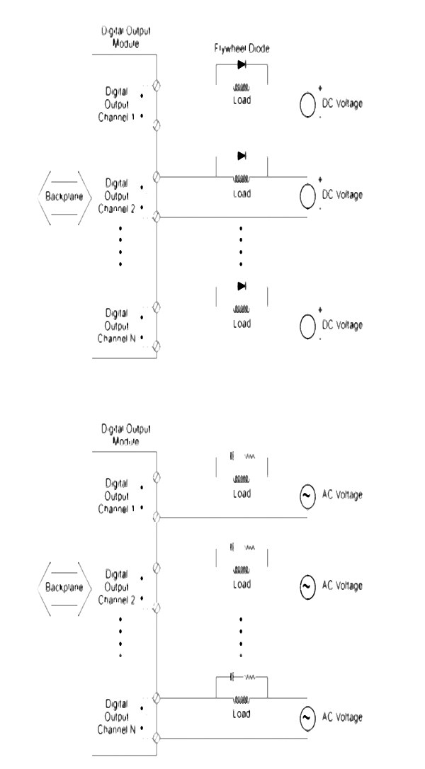
Flywheel diode or RC circuit for digital outputs
14.3 Master site structure
The central site/master station can be pictured as having one or more operator stations (tied together with a local area network) connected to a communication system consisting of modem and radio receiver/transmitter. It is possible for a landline system to be used in place of the radio system; in this case the modem will interface directly to the landline. Normally there are no input/output modules connected directly to the master stations although there may be an RTU located in close proximity to the master control room.
The features which should be available are:
- Operator interface to display status of the RTUs and enable operator control
- Logging of the data from the RTUs
- Alarming of data from the RTU
Master stations
A master station has two main functions:
- Obtain field data periodically from RTUs and sub-master stations
- Control remote devices through the operator station
There are various combinations of systems possible, as indicated in Figure 14.11 below.
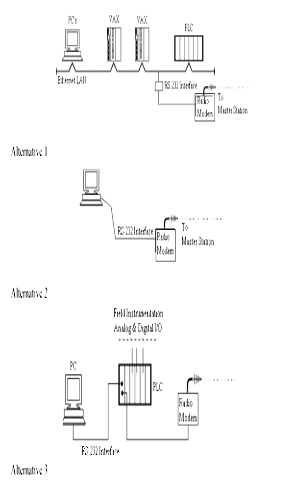
Various approaches Possible for the master station
It may also be necessary to set up a sub-master station. This is to control sites within a specific region. The sub-master station has the following functions:
- Acquire data from RTUs within the region
- Log and display this data on a local operator station
- Pass data back to the master station
- Pass on control requests from the master station to the RTUs in its region (see Figures 14.12 and 14.13)
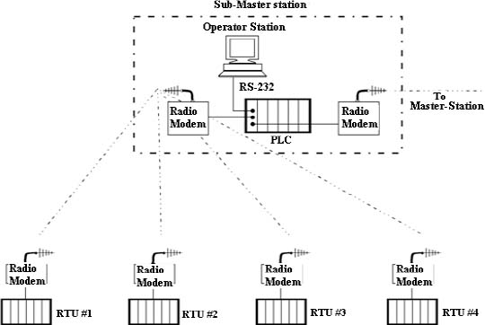
Sub-master architecture
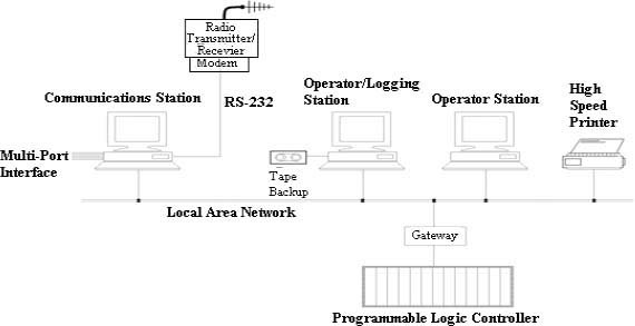
Typical structure of the master station
The master station has the following typical functions:
- Establishment of Communications:
- Configure each RTU
- Initialize each RTU with input/output parameters
- Download control and data acquisition programs to the RTU
- Operation of the Communications Link:
- If a master slave arrangement, poll each RTU for data and write to RTU
- Log alarms and events to hard disk (and operator display if necessary)
- Link inputs and outputs at different RTUs automatically
- Diagnostics:
- Provide accurate diagnostic information on failure of RTU and possible problems
- Predict potential problems such as data overloads
Master station software
There are three components to the master station software:
- The operating system software
- The system SCADA software (suitably configured)
- The SCADA application software
There is also the necessary firmware (such as BIOS) which acts as an interface between the operating system and the computer system hardware.
The operating system software will not be discussed further here. Good examples of this are DOS, Windows, Windows NT and the various UNIX systems.
System SCADA software
This refers to the software put together by the particular SCADA system vendor and then configured by a particular user. Generally it consists of four main modules:
- Data acquisition
- Control
- Archiving or database storage
- The Man Machine Interface (MMI)
A successful SCADA system design implies considerable emphasis on the central site structure.
In this chapter we will discuss the fundamentals of SCADA software and its configuration. SCADA packages and their interface are given. The important components of SCADA are highlighted.
Learning objectives
- Fundamentals
- Components of a SCADA system
- Software – design of SCADA packages
- Configuration of SCADA systems
- Building the user interface
15.1 Fundamentals
SCADA software can be divided into two types, viz. proprietary or open. Companies develop proprietary software to communicate to their hardware. These systems are sold as ‘turn key’ solutions. The main problem with these systems is the overwhelming reliance on the supplier of the system. Open software systems have gained popularity because of the Interoperability they bring to the system. Interoperability is the ability to mix different manufacturers equipment on the same system.
The SCADA software performs the following functions:
- User interface
- Graphics display
- Alarms
- Trends
- RTU (and PLC) interface
- Scalability
- Access to data
- Networking
Examples of modern SCADA software include Citect, Wonderware, and Proficy, to name but a few.
15.2 Components of a SCADA system
The typical components of a SCADA system with emphasis on the SCADA software are indicated in the diagram below. Figure 15.1 shows the components of SCADA.
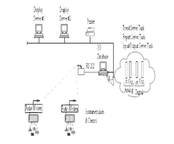
Components of a SCADA system
Typical key features expected of the SCADA software are listed below. Naturally these features depend on the hardware to be implemented.
15.2.1 SCADA key features
The SCADA system’s features differ between manufacturers, but the basic concept remains the same. The general features of SCADA include user interfaces, graphical displays, alarms, trends, RTU interfacing, a data historian, and networking. Some of the general features of SCADA are listed below with examples.
User interface:
- Keyboard
- Mouse
- Trackball
- Touch screen
Graphics displays:
- Customer-configurable, object-orientated, and bit-mapped
- Unlimited number of pages
- Resolution: up to 1280 × 1024
Alarms:
- Client server architecture
- Time stamped alarms to 1 ms precision (or better)
- Single network acknowledgement and control of alarms
- Alarms are shared with all clients
- Alarms displayed in chronological order
- Dynamic allocation of alarm pages
- User-defined formats and colours
- Up to four adjustable trip points for each analogue alarm
- Deviation and rate of change monitoring for analogue alarms
- Selective display of alarms by category
- Historical alarm and event logging
- Context-sensitive help
- On-line alarm disabling and threshold modification
- Event-triggered alarms
- Alarm-triggered reports
- Operator comments can be attached to alarms
Trends:
- Client server architecture
- Zooming
- Export data to DBF, CSV files
- X/Y plot capability
- Event-based trends
- Pop-up trend display
- Trend grid lines or profiles
- Background trend graphics
- Real-time multi-pen trending
- Short- and long-term trend display
- Length of data storage and frequency of monitoring specified on a per-point basis
- Archiving of historical trend data
- On-line change of time-base without loss of data
RTU (and PLC) interface:
- All compatible protocols included as standard
- DDE/OPC drivers supported
- Interface also possible for RTUs, loop controllers, bar code readers, and other equipment
- Driver tool kit available
Scalability:
- Additional hardware can be added without replacing or modifying existing equipment
- Limited only by the PLC architecture (typically 300 to 40,000 points)
Access to data:
- Direct, real-time access to data by any network user
- Third-party access to real-time data, for example, lotus 123 and excel
- Network DDE/OPC access to data
- ODBC driver support
- Direct SQL commands for high-level reporting
Networking:
- Support of all major operating systems
- Centralized alarm, trend, and report processing – data available from anywhere in the network
- Dual networks for full LAN redundancy
- No network configuration required (transparent)
- Multi-user system, full communication between operators
- WAN supported with high performance
- PSTN dial-up support
15.3 Software- design of SCADA packages
While performance and efficiency of the SCADA package with the current plant is important, the package should be easily upgradeable to handle future requirement. The system must be easily modifiable as the requirement change and expandable as the task grows, in other words the system must use a scaleable architecture.
There have been two main approaches to follow in designing the SCADA system in the past. They are centralized and distributed.
Centralized: where a single computer or mainframe performs all plant monitoring and all plant data is stored on one database that resides on this computer. The disadvantages with this approach are simply:
- Initial up front costs are fairly high for a small system
- A gradual (incremental) approach to plant upgrading is not really possible due to the fixed size of the system
- Redundancy is expensive as the entire system must be duplicated
- The skills required of maintenance staff in working with a mainframe type computer can be fairly high. (Figure 15.2 shows the centralized processing)
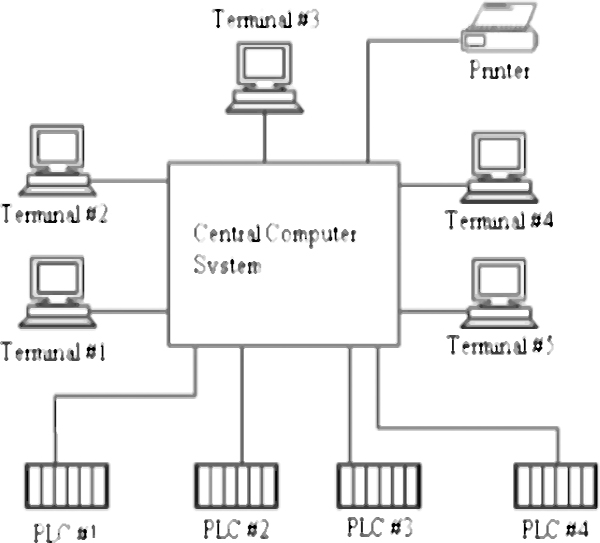
Centralized processing
Distributed: where the SCADA system is shared across several small computers (usually PCs) (See figure 15.3). Although the disadvantages of the centralized approach above are addressed with a distributed system, the problems are:
- Communication between different computers is not easy, resulting in configuration problems
- Data processing and databases have to be duplicated across all computers in the system, resulting in low efficiencies
- There is no systematic approach to acquiring data from the plant devices – if two operators require the same data, the RTU is interrogated twice
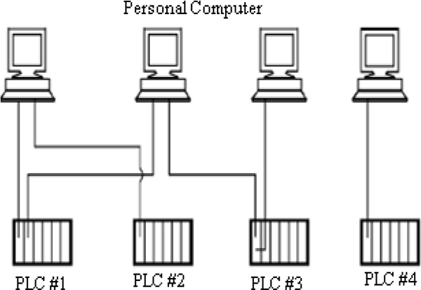
Distributed processing
An effective solution is to examine the type of data required for each task and then to structure the system appropriately. A client server approach also makes for a more effective system.
A client server system is understood as follows: A server node is a device that provides a service to other nodes on the network. A common example of this is a database program. A client on the other hand is a node that requests a service from a server. The word client and server refer to the program executing on a particular node.
A good example is a display system requiring display data. The display node (or client) requests the data from the control server. The control server then searches the database and returns the data requested, thus reducing the network overhead compared to the alternative approach of the display node having to do the database search itself. A typical implementation of a SCADA system is shown in the figure 15.4.
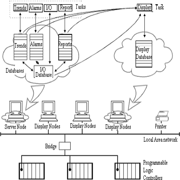
Client server approach as applied to a SCADA system
There are typically five tasks in any SCADA system. Each of these tasks performs its own separate processing.
Input/output task:
- This program is the interface between the control and monitoring system and the plant floor
Alarm task:
- This manages all alarms by detecting digital alarm points and comparing the values of analogue alarm points to alarm thresholds
Trends task:
- The trends task collects data to be monitored over time
Reports task:
- Reports are produced from plant data. These reports can be periodic, event triggered or activated by the operator
Display task:
- This manages all data to be monitored by the operator and all control actions requested by the operator
A large system with 30 000 points could have architecture as indicated in figure 15.5.
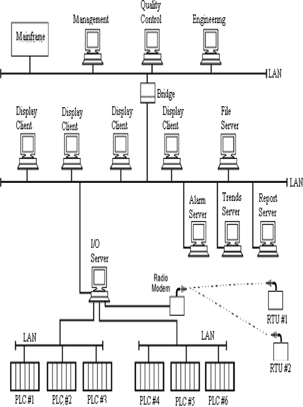
A large SCADA application
Redundancy
A typical example of a SCADA system where one component could disrupt the operation of the entire system is given in the figure 15.6.
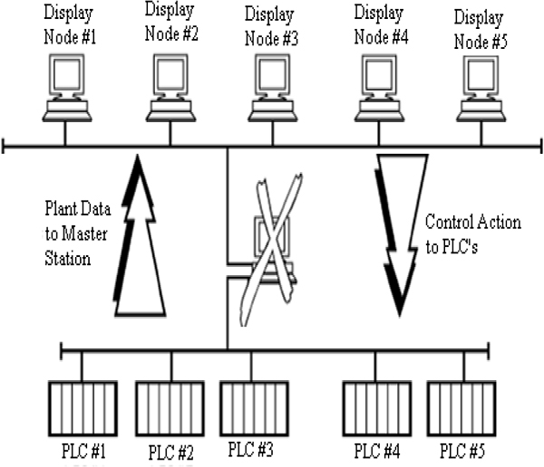
The weak link
If any processes or activities in the system are critical, or if the cost of loss of production is high, redundancy must be built into the system.
This can be done in a number of ways as indicated in the following diagrams. The key to the approach is to use the client–server approach, which allows for different tasks (comprising the SCADA system) to run on different PC nodes. For example, if the trend task were important, this would be put in both the primary and secondary servers. Figure 15.7 shows the duty server redundancy.
The primary server would constantly communicate with the secondary server updating its status and the appropriate databases. If the primary server fails, the standby server will then take over as the primary server and transfer information to the clients on the network. Figure 15.8 shows dual LANs and PLCs.
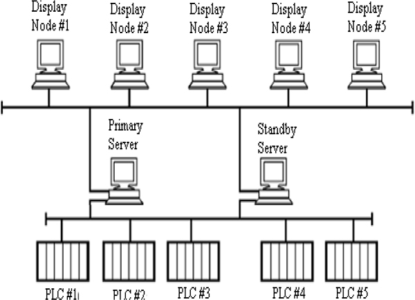
Dual server redundancy
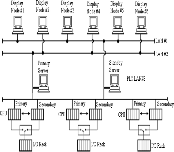
Dual LANs and PLCs
System response time
These should be carefully specified for the following events. Typical speeds that are considered acceptable are:
- Display of analogue or digital value (acquired from RTU) on the master station operator display (1 to 2 seconds maximum)
- Control request from operator to RTU (1 second critical; 3 seconds noncritical)
- Acknowledge of alarm on operator screen (1 second)
- Display of entire new display on operator screen (1 second)
- Retrieval of historical trend and display on operator screen (2 seconds)
- Sequence of events logging (at RTU) of critical events (1 millisecond)
It is important that the response is consistent over all activities of the SCADA system. Hence the above figures are irrelevant unless the typical loading of the system is also specified under which the above response rates will be maintained. In addition no loss of data must occur during these peak times. A typical example of specification of loading on a system would be:
- 90% of all digital points change status every 2 seconds (or go from healthy into alarm condition).
- 80% of all analogue values undergoing a transition from 0 to 100% every 2 seconds.
The distributed approach to the design of the SCADA system (where the central site/master station does not carry the entire load of the system) ensures that these figures can be easily achieved.
Expandability of the system
A typical figure quoted in industry is that if expansion of the SCADA system is anticipated over the life of the system the current requirements of the SCADA system should not require more than 60% of the processing power of the master station and that the available mass storage (on disk) and memory (RAM) should also be approximately 50% of the required size. It is important to specify the expansion requirements of the system, so that;
- The additional hardware that will be added will be of the same modular form, as that existing and will not impact on the existing hardware installed
- The existing installation of SCADA hardware/control cabinets/operator displays will not be unfavourably impacted on by the addition of additional hardware. This includes items such as power supply/air conditioning/SCADA display organization
- The operating system will be able to support the additional requirements without any major modifications
- The application software should require no modifications in adding the new RTUs or operator stations at the central site/master station
15.4 Configuration of SCADA systems
15.4.1 Common pitfalls of SCADA
There is a vast array of SCADA and telemetry equipment available on the market, servicing everything from small low-integrity applications to large sophisticated systems. Before attempting to specify a system, it is best to visit and inspect as many different telemetry suppliers as possible. This will provide a good feeling for the levels of systems available and help evaluate the level of equipment suitable for the application.
It is important not to expect too much from the equipment unless you are willing to pay for it. Over-specifying a system, by asking for more than what is really needed, can see a project fail because of blowouts in budgets. If a particular feature is not required at present, but may be in the future, do not specify it as a requirement initially, but include a requirement that the system should be easily expandable at any time to include the feature.
The other major pitfall is not specifying the complete system. Do not assume that a feature is included in the equipment because it says so in the manufacturer’s literature. Write every trivial technical requirement into the specification. Before writing the specification, do a thorough survey of the application. Talk to all relevant personnel who will be involved in the implementation, management, and maintenance of the system. Carefully list every requirement in the tender document.
A further consideration is the choice of communications medium. Do not assume that the general vendor information will necessarily be true for your application (they have vested interests). Do a careful budgetary analysis of different mediums. Ensure that the medium can provide the quality of data transmission required. Obtain budgetary prices and performance specifications of equipment and services from suppliers prior to tender to help evaluate the best medium. Where possible, visit a number of installations to evaluate how they are performing.
15.4.2 OPC and the need for a data exchange standard
OPC originally stood for Object Linking and Embedding (OLE) for Process Control. Since OLE has been superseded by “ActiveX,” this acronym has become meaningless and consequently “OPC” has become just a name. It is sometimes said to represent “Openness, Productivity, and Connectivity.”
OPC is an open, standards-based infrastructure for the exchange of process control data and specifies a set of software interfaces for several logical (software) objects, as well as the methods (functions) of those objects. It is a software standard supported by all major SCADA vendors, and most OPC products (clients and servers) operate very much in an “out-of-the box, plug-and-play” fashion. If they so wish, users can develop their own clients and servers by means of developers’ toolkits. It is even possible to develop simple HMI systems without any programming knowledge at all.
The scope of OPC is to focus primarily (though not exclusively) on the exchange of “raw” data, that is, the efficient reading and writing of data between an application and a process control device. In other words, OPC is a “window” through which plant data can be observed. It accomplishes this by specifying the “rules” for the data exchange in sufficient detail to allow vendors to implement low level (i.e. software) interfaces to process data.
There are, however, certain implementation issues not addressed by OPC (albeit deliberately). These include:
- Hardware interconnection. The protocol issues (drivers etc) for the I/O subsystems are not covered by the OPC specifications, and have to be taken care of by the server vendors
- How clients and servers are to be implemented. Apart from specific guidelines in the OPC specifications and strict adherence to the interface definitions, vendors can implement clients and servers in any way they want. As a result, OPC products differ in terms of speed, reliability, and interoperability
The goals of the original OPC Task Force was to develop a way to facilitate easy access to process data. The system had to be easy to use, easy to implement (especially on the server side), had to operate efficiently in terms of the usage of system resources (such as CPU usage), had to have a reasonably high level of functionality, and had to be flexible enough to accommodate the needs of multiple vendors. These goals were met, and the original “OPC Task Force” (1995), representing Fisher-Rosemount, Intellution, Intuitive Technology, Opto22, Rockwell Automation, Siemens, and Microsoft has grown into the present OPC Foundation with several thousands of members. Figure 15.9 shows the OPC foundation logo.

OPC foundation logo
15.4.3 The problems addressed by OPC
Process control architectures
Most of the problems addressed by OPC can be traced back to the use of a multi-layered process control architecture and a heterogeneous computing environment.
Automation systems provide users with three primary services namely control, configuration, and data collection. Control involves the exchange of time-critical data between controlling devices such as PLCs and I/O devices such as actuators and sensors. Networks that are involved in the transmission of this data must provide some level of priority setting and/or interrupt capabilities, and should behave in a fairly deterministic fashion, depending on the specific application.
The second type of functionality, namely configuration, typically involves a personal computer or a similar device in order for users to set up and maintain their systems. This activity is typically performed during commissioning or maintenance operations, but can also take place during runtime, for example, recipe management in batch operations.
The third involves the collection of data for the purposes of display (e.g. in HMI stations), data analysis, trending, troubleshooting, or maintenance.
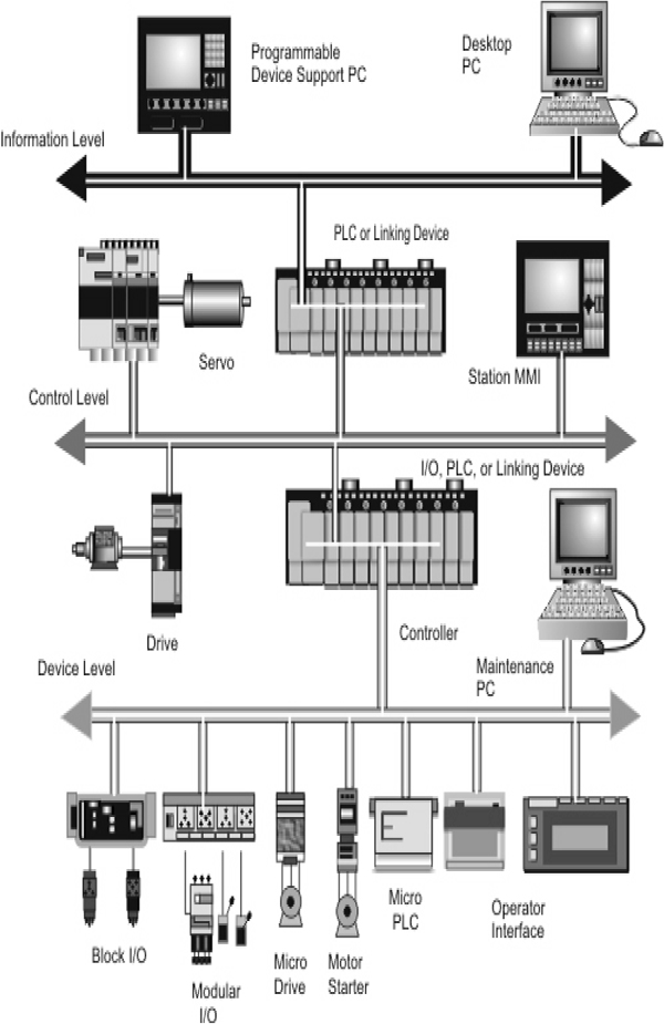
Hierarchy of plant levels
Figure 15.10 shows a generic view of automation system architecture. At the device level, information is exchanged primarily between devices and networks deployed on the plant floor. Fast cycle times are required, networks at this level are bit-or byte oriented, and data packets are fairly small. Examples are HART, AS-i, DeviceNet, PROFIBUS DP, and Foundation Field bus H1. These are mostly bit-or byte oriented network technologies and are generically referred to as “field buses.”
At the control level, data is primarily exchanged between HMIs and PLCs. At this level, speed is less critical and the amount of data exchanged in a packet is, generally speaking, bigger. These systems at this level are said to be message oriented, and the examples are ControlNet and Foundation Field bus HSE.
At the information level, we find larger computers (e.g. mainframes) often networked via Token Ring or Ethernet, often at up to 10 Gbps speeds. Here, determinism is not a factor. However, at this level, there could be a large number of different operating systems such as Windows, UNIX, and LINUX.
The current trend is for vendors to repackage their older systems by running them via a TCP/IP stack over Ethernet, and these systems are used in the device as well as at the control level.
Problems arising from the process control architecture
Various categories of personnel, from operators to the CEO, need to access data across all three layers at various points in time. This is difficult or almost impossible due to various factors, relating to the data sources, data formats, data users, the interconnection between data sources and data users, and operating systems. These will now be discussed in more detail.
Data sources
Data sources could include (but are not limited to computers, databases (e.g. SQL), PLCs, DCSs, Stand-alone (e.g. PID) controllers, and RTUs. Each of these could use a different protocol at layer 7 of the OSI model. Even if they were all interconnected via the same physical network, the interrogating (client) system would need to be able to converse via several protocols.
Data format
Data format is another problem area. The data source (e.g. RTU) could, for example, make its data available in one of the following formats: Boolean (single bit), character (signed 8-bit), word (unsigned 16-bit), short (signed 16-bit), dword (unsigned 32-bit), long (signed 32-bit), BCD (2-byte packed BCD), LBCD (4-byte packed BCD), float (32-bit floating point number), double (64-bit floating point number), or string (null terminated ASCII string). The client software would need to accommodate all of these.
Data users
The plant data obtained from various sources could end up being used by multiple clients. These could include HMIs, SCADA servers, and data historians.
This data might be used for functions such as reporting, operator interfacing, trending, alarming, or control strategies. Depending on the application, the data could be accessed in groups or per individual items. It could either be polled by the client at constant intervals or be forwarded by the server to the client on an exception basis.
Interconnections
Interconnections, especially between server host and I/O device, could be varied. Technologies and standards employed could include:
- Point-to-point links utilizing fibre, RS-232, RS-422, Bell-202 type modem links, and 900 MHz/2.4 GHz microwave links, to name but a few multi-drop buses
- Options here include RS-485 and IEC 61158 protocols
- Options include Modbus, DNP3, and DF-1, to name but a few networks
- Most networks nowadays use Ethernet at OSI layers 1 and 2, and TCP/IP at OSI layers 3 and 4
Operating systems
This is another problem area. The various operating systems used server as well as client hosts could vary between Windows (95/98/NT, 2000, XP, CE, 2003, etc.), UNIX, LINUX, and various real-time operating systems for embedded controllers.
Drivers
The figure 15.11 shows a simplified example of a high-speed rotating machine control system.
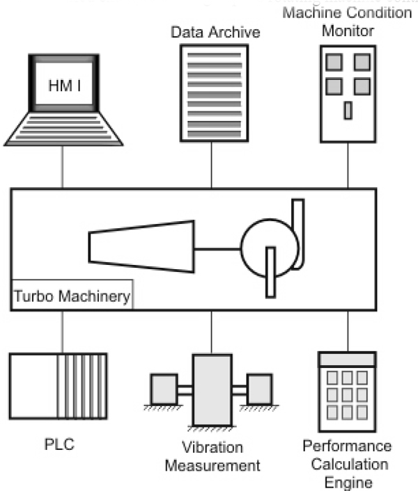
Control system example
The lower portion of the diagram shows three independent control systems, each serving as a data source. They are:
- A PLC for interlocking operations and for supervision of vital operating parameters
- A vibration instrument that measures machine vibration
- A vendor-supplied performance calculation engine
The PLC will be connected to several I/O devices for control of the machine, using its own standard interfaces and communication protocols. All these are essentially self-contained devices that may include their own HMI hardware or other form of output devices such as hardwired indicators, annunciators, and so on. However, they are also required to communicate with other devices provided for overall control of the process itself, of which this particular machine is a component.
The upper portion of the diagram shows three such devices:
- An HMI used by the process control operator for obtaining the system status, the alarm conditions when there is an undesirable deviation from specific threshold values, and often for control of the process
- A data archive for storing various measured values, events, etc.
- A machine condition monitoring system
Assume that all data sources and data users shown in this example are proprietary systems. We can see right away that there is a need for each of the data user devices to obtain data from each of the data sources shown here. For example, the HMI will need status and alarm data from the PLC. It will also require vibration readings and critical alarms in the event of excessive vibration values for operator information. It will need interaction with the calculation engine to display critical calculated parameters to the process operator and use the results as inputs to say, an expert system application for operator guidance. The same will be true of the data archive device and the machine monitoring system. Figure 15.12 shows the Communication between proprietary systems using separate drives.
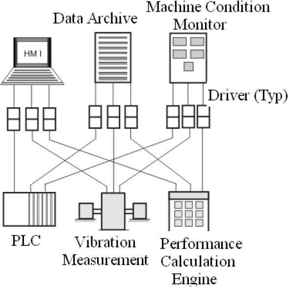
Communication between proprietary systems using separate drivers
With all these systems being proprietary in nature, direct communication between any two devices is impossible without some customized interfacing. The HMI will need an interface to access the data residing in the PLC. Similarly, it will need another interface to access the data from the vibration measuring instrument, and so on. Each interface is a special purpose software application known as a device driver (simply referred to as a “driver”). Each connection between two devices thus calls for two dedicated custom-developed drivers, one at each end. These cannot be used with any other device, and even between a pair of devices the driver may need to be rewritten if the data source or the data-using device is replaced or upgraded.
There is also another less obvious problem. Each data source device has to communicate through multiple drivers to the data users. This means that identical data may be requested by multiple user devices and has to be communicated separately to each by the data source. With slow serial protocols such as Modbus Serial, such a requirement puts a severe strain on the communication infrastructure. Thus, we need nine device drivers in this scenario, each will have to be custom-developed, and each may become useless if any of the corresponding devices is replaced or even upgraded.
The result is a lack of interoperability, getting locked-in to specific vendors, and time-consuming software development and on-going management. Such a situation is neither in the user’s interest, because of the difficulties cited above, nor in the manufacturers’ interest, because they are the ones expected to supply the drivers. It is thus obvious that we can arrive at a “win-win” situation by making all devices talk in a common language. Let us now modify the example in the previous figure with another, representing communication through such a common language. This is shown in the figure 15.13.
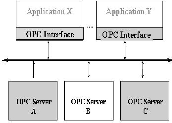
Communication between proprietary systems via OPC
In this scenario, each data source has a software component for making its data available to other systems (let us call it the “server”) and each data user has a software component to access the server for data (let us call this the “client”). We have therefore created a “software bus.” By adopting a common data interface standard, it is possible for any client to request data from any server in a format that the server can understand. The server, in turn, makes the requested data available to the client in a format that the client can understand. As long as the client and server applications are all based on a common specification, any client and any server can thus exchange data thereby ensuring interoperability.
Since there is no proprietary component in this data exchange mechanism, it automatically ensures vendor independence. Scalability, too, is not an issue since a new data source following the same data exchange specification can easily be added. Device upgrades pose no problem either since the data exchange mechanism will still be based on the same common standard. Server vendors are also not required to develop drivers to suit various client products, but simply have to implement the required OPC interfaces.
The OPC logical object model
It is, strictly speaking, inappropriate to talk about a logical (i.e. software) object model for OPC as each specification has a different object structure. In other words, there is a DA object model, an AE object model, etc. This is, in fact, considered a shortcoming and is being addressed by the new UA standards. We will clarify the concept be looking at the most popular specification to date, the DA (Data Access) specification. Initially this was known simply as “OPC Specification.”
There can be a one-to-one relationship between the client and the server, or, alternatively, there can be a one-to-many or many-to-one relationship between them as shown in the following figure. However, although multiple client–server connections are possible, this is dependent on specific vendor implementations and hence not always possible. Figure 5.14 shows the relation between the client and the server.
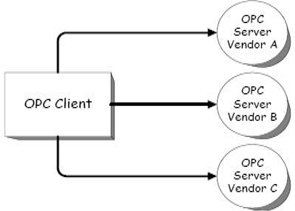
Basic relationship between OPC clients and servers
OPC Clients and Servers are simply software “objects.” The connection between the client and the server is via well-defined interfaces, specified in Microsoft Interface Definition Language (IDL) and typically implemented in C++. A typical interface specification would only make sense to a programmer. The infrastructure to carry the data between the client and the server interfaces was initially supplied by Microsoft DCOM, but DCOM is now being phased out in favour of the .NET (dot Net) infrastructure.
A more complex client–server relationship is shown in the figure 15.15. Here, the client (A) obtains data from the server (B) via an OPC interface. The server, in turn, obtains I/O data from a device (e.g. a PLC), shown as C. The channel between the server and the device could, for example, be Ethernet or RS-485, and the server vendor would develop the device drivers in consultation with the device vendor. In this specific scenario, there is also a SCADA system that obtains its own data via an I/O subsystem (D). If the SCADA system is OPC compatible, that is, if it has a built-in OPC server, then OPC server B could obtain data directly from the OPC server on the SCADA system via OPC Bridging software. Obviously, this indirect method of obtaining data would be an issue if fast access to the plant data is a prerequisite.
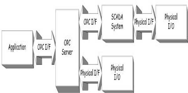
More complex relationship between OPC clients and servers
When “looking inside” an OPC Server such as an OPC DA (Data Access) Server, the internal structure of the server becomes evident. The structure varies from specification to specification, but there is always a single Server control object at the top. In the case of DA, this object has the very creative name of OPC Server (note the absence of a space after OPC). Below this are one or more OPC Group objects, and below each of these is one or more OPC Item objects. The Interfaces of the OPC Server and OPC Group objects extend to the outside world, but those of the OPC Items do not, and as a result, a Client can only be interrogated the items indirectly via the OPC Group interfaces. Figure 15.16 shows the internal structure of DA server.
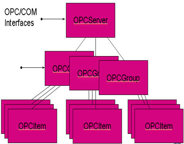
Internal structure of DA server
Incidentally, one of the drawbacks of the first generation of OPC specifications is that they are not built around a coherent data model, that is, the object hierarchy of a DA server is different to that of an AE (Alarms and Events) server. This has been addressed by the new OPC Unified Architecture (AU).
15.5 Building the user interface
15.5.1 HMI interface overview and control techniques
HMI is the most important component of any monitoring and control system. A properly-designed HMI will ensure that the system is easy to navigate and monitored parameters are displayed logically on the screen.
HMI provides a graphical user interface which provides an operator with easy status viewing and control. It also records events and maintains a database regarding it which can be used by the graphical user interface.
Mimics (overview to bay level)
In the figure 15.17, the HMI has a default screen showing an overall substation mimic depicting the status of primary transmission lines, selected measured values and indication of the presence of alarm conditions and their locations. The default screen also displays an overall event record window showing all substation events and their time stamps in chronological order.
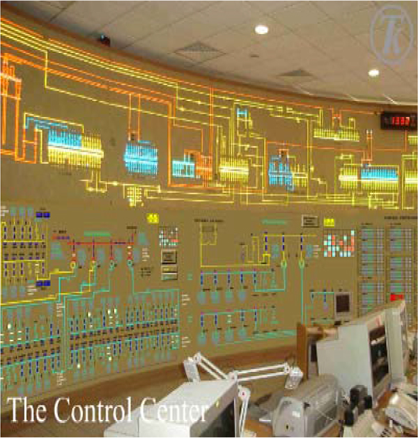
Substation Transmission lines and Feeders mimic (Source: http://www.telecont.com/)
It is possible to drill down into any bay to see the details of any mimic for the bay with measured values and alarm status. The operation and maintenance of the primary transmission lines is carried out from here. The bay level screen is also required to display a bay-specific event record window showing all events related to the particular bay and their time stamps in chronological order.
The Substation Automation would provide control and monitoring of the various equipment. This is at two levels viz.:
- At the individual bay level
- At the HMI level in the central control level.
The following are the bay level functions:
- Functions related to bay control
- Functions related to bay protection
- Functions related to bay metering
Control
It must be kept in mind that SCADA systems perform only supervisory (i.e. high-level control) control. For example, on closed-loop control systems (PID control) they are used to change the set point, but do not perform the actual control.
Set points can be altered by displaying the PID controller faceplate, and dragging the set point indicator with the mouse or pointing device. Alternatively on/off switching can be performed either by clicking on the switch icon on the screen, or touching it in the case of a touch-sensitive screen.
A third option for on/off control or set point variation is to perform it remotely via OPC, provided that the operator has the required login credentials.
Alarm displays
Alarm systems are an integral part of HMI. An alarm system consists of both hardware and software including field signal sensors, transmitters, alarm generators and handlers, alarm processors, alarm displays, annunciator window panels, alarm recorders and printers. In configuring an alarm system the following issues need to be addressed.
- The purpose of each proposed alarm and for what hazards or risks it will provide a warning to the operator needs to be known. The consequences of alarm failure or the alarm being overlooked need to be identified. If the proposed alarm provides only information of an event/incident, then it should not be configured as an alarm.
- Assessment of the severity of the risk in terms of potential loss of life or injury, economic losses, environmental impact and substation damages must be done. Any hazard to people should be identified by a formal risk assessment. Economic risks, potential substation damages or losses of revenue should be expressed in monetary terms.
- It must be known whether there are any protection systems in the line to provide protection against the risk, and whether an automatic protection system can be used with or without configuring the alarm.
- It must be established whether an alarm is safety-related or not. If an alarm is not safety-related, then the economic and/or environmental risks involved in implementing the alarm within the process control system should be known. Safety-related alarms should be implemented outside the process control system, unless the control system itself is safety-related. At times there may be ergonomic advantages along with reliability reasons for displaying some economic/environmental significant alarms on individual or standalone alarm annunciators.
Alarm Window
All process or system-related alarms are logged as and when they happen, and are displayed in the Alarm screen area. Normally, alarms are defined group wise, with the groups being decided on as per process sections. Figure 15.18 shows a typical layout of Alarm screen.
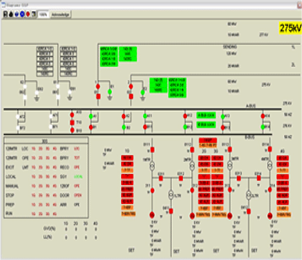
Alarm screen layout
An alarm screen shows an alarm along with other necessary information, such as date and time when it occurred and whether or not it has been acknowledged or reset (and when), etc. This feature enables the user to check the alarm history of the past few days.
Alarm processing is an important part of the operator station. Error codes identifying the faults are normally included with the description of the failed device.
No other part of the operator display has as much impact on the health of the transmission substations and on the operator. The alarm function should be viewed as an integral part of the operator interface and not as a standalone feature. Figure 15.19 shows the alarm actions in an operator display.
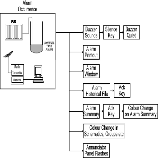
Alarm actions in an operator display
As a rule of thumb, only four alarm priorities should be implemented. These are:
- High Priority
- Alarms that give warning of dangerous conditions that could cause a shutdown of a major activity
- Medium Priority
- Alarms that should be acted on as quickly as possible, but will not cause a shutdown
- Low Priority
- Alarms that should be dealt with when time permits
- Event Only
- Information of a statistical or technical nature. No annunciation sounds are required for these
The number and types of alarms should be limited is in order to keep the system straightforward and ensure easy interpretation of all alarms. Higher-priority alarms should be louder, lower-pitched and have a higher pulse frequency than the lower priority alarms. Alarms should be classified as unacknowledged (and flashing on the screen) until the operator acknowledges them via the keyboard. They then become an accepted alarm. One weakness in many systems is the occurrence of trivial alarms, which may irritate and confuse the operator. The table 15.1 gives a list of trivial alarms.
| TYPE OF ALARM | SYMPTOM | REMEDY |
|---|---|---|
| Consequential | Repetitive alarms caused by a condition that the operator is aware of. | Inhibit the alarm until the condition is remedied. |
| Out of service | Alarms caused by equipment not in service | Inhibit the alarms |
| No action alarms | Operator unable to rectify the problem | Delete the alarm from the system |
| Equipment changes | Regular equipment maintenance etc. causes alarms | Ensure the alarms are suppressed for this period by added alarm logic. |
| Minor event | Operator constantly being notified about trivial events | Delete alarm and replace with event recording. |
| Multiple | Many alarms triggered by one fault | Use first up alarming to reduce the alarm information. |
| Cycling | Signal close to alarm level moves the alarm in and out of alarm condition. | Expand the range of signal before moving into alarm |
| Instrument drift | Drift of instrument causes alarm | Ensure there is tight control on the calibration of instruments |
A guiding principle is that alarms should be both relevant and timely. An operator’s time should not be wasted by presenting a plethora of useless alarms. It is important to continuously audit, maintain and improve on the performance of the alarm system through analysis and review, with the involvement of the operators. The following should be documented for every alarm:
- Type of alarm
- Alarmed tag
- Description of tag
- Reasons for alarm
- Relationship to related alarms (consequential relationships)
- Description of the logic in the generation of the alarm
- Possible causes of the alarm
- Action steps to take to remedy the alarm situation
Alarms should be able to be disabled provided the operator has the relevant key. Suggested colours for alarms could be:
- Red – high priority
- Magenta – medium priority
- Yellow – low priority
Trend displays
The HMI processes the operational data associated with the process to determine a trend in the operational data. The graphical representation of the trend is displayed by the user interface. The trend display may be modified by:
- Expanding the graphical representation of the trend
- Compressing the graphical representation of the trend
- Changing a scale of the graphical representation of the trend
- Removing a portion of the graphical representation of the trend
Trend window
These displays occupy part of, or the complete screen depending on the configuration. They provide trends on the data of analogue process variables. Figure 15.20 shows the trend screen layout.
Trend screen layout (Courtesy: ABB)
Along with the trends of process parameters, it offers different tools such as zoom in, zoom out, ruler, X-Y plot, etc., to facilitate analysis of different process parameters. These features are very useful from operational and maintenance points of views.
Trend tags have to be defined along with scan time or logging time, which are freely configurable. It is one of the important criteria whilst selecting HMI software, since different software packages have different ranges for logging time.
In this chapter we will discuss twisted pair cables, fibre optic cables, public network provided services, industrial Ethernet, different protocols TCP/IP, Fieldbus, MODBUS, LAN connectivity via Bridges, Routers, Switches, and the importance of SCADA network security.
Learning objectives
- Twisted pair cables
- Fibre optic cables
- Public network provided services
- Industrial Ethernet
- TCP/IP
- Fieldbus
- MODBUS
- LAN connectivity
- Bridges
- Routers
- Switches
- SCADA network security
16.1 Twisted pair cables
Twisted pair cables are the most economical solution for data transmission and allow for transmission rates of up to 1 Mbps on communication links of up to 300 m (longer distances with lower data transfer rates). Some new types of twisted pair cables (e.g. Twistlan) are suitable for up to 10 Mbps. Twisted pairs can be STP (shielded twisted pair) or UTP (unshielded twisted pair).
Tests have recently been carried out in a factory environment where speeds of 100 and 200 Mbit/s were successfully run over twisted pairs. It is expected that 500 Mbit/s systems will be commercially available within the next few years. It has also been reported that successful laboratory trials have been carried out at a 1 Gbps over very short distances.
Twisted pairs are made from two identical insulated conductors, which are twisted together along their length at a specified number of twists per meter, typically 40 twists per meter (12 twists per foot). The wires are twisted to reduce the effect of electromagnetic and electrostatic induction. An earth screen and/or shield are often placed around them to help reduce the electrostatic (capacitive) induced noise. An insulating PVC sheath is provided for overall mechanical protection. The cross-sectional area of the conductor will affect the IR loss, so for long distances thicker conductor sizes are recommended. The capacitance of a twisted pair is fairly low at about 10 to 50 pF/ft, allowing a reasonable bandwidth and an achievable slew rate.
For full-duplex digital systems using balanced differential transmission, two sets of screened twisted pairs are required in one cable, with individual and overall screens. A protective PVC sheath then covers the entire cable.
Due to the rapid increase during the 70s and 80s of twisted pair cables in data communications applications, the EIA developed a structured wiring system for unshielded twisted pair (UTP) cables. This structure provides a set of rules and standards for the selection and installation of UTP cables in data communications applications up to 100 Mbit/s.
The structure involves dividing UTP into five categories of application. These are listed below:
- CATEGORY 1 UTP – Low speed data and analogue voice
- CATEGORY 2 UTP – ISDN data
- CATEGORY 3 UTP – High speed data and LAN
- CATEGORY 4 UTP – Extended distance LAN
- CATEGORY 5 UTP – Extended frequency LAN
The following table shows the electrical characteristics defined for the cables and connectors used with Categories 3, 4 and 5 UTP.
| Category 3<=10 MHz |
Category 3>=10 MHz |
Category 4<=10 MHz |
Category 4>=10 MHz |
Category 5<=10 MHz |
Category 5>=10 MHz |
Category 5<=100 MHz |
|
|---|---|---|---|---|---|---|---|
| Connector Attenuation (dB) | 0.4 | 0.4 | 0.1 | 0.2 | 0.1 | 0.2 | 0.4 |
| Cable Impedance (ohms) | 100 | 100 | 100 | 100 | 100 | 100 | 100 |
| Cable Attenuation (dB/km) | 26 (1MHz)98 (10Mz) | 131 | 21 (1MHz) 72 (10Mz) | 89 (16Mz) 102 (20Mz) | 20 (1MHz) 6.6 (10Mz) | 82 (16Mz) 92 (20Mz) | 220 |
| Patch Cord Impedance (ohms) | 100 | 100 | 100 | 100 | 100 | 100 | 100 |
| Patch Cord Attenuation (dB/km) | 25 (1MHz)98 (10Mz) | 131 | 26 (1MHz) 98 (10Mz) | 131 | 26 (1MHz) 98 (10Mz) | 131 | 131 |
The connection point of a landline into a building or equipment shelter is at the main distribution frame (MDF) or intermediate distribution frame (IDF).
In making data connections to modems, telemetry units or computer equipment, it is common to use withdrawable multiconductor connectors (e.g. 9-pin, 15-pin, 25-pin, 37- pin, 50-pin, etc). These connectors are usually classified as follows:
- The type, make or specification of the connector
- The number of associated pins or connections
- The gender (male or female)
- Mounting (socket or plug)
For example, the well known connector DB-25 SM specifies a D-type, 25 pin socket, male (with pins).
There are many different types of connectors used by computer manufacturers such as IBM, Hewlett Packard, Wang, Apple, etc and the various manufacturers of printers, radio equipment, modems, instrumentation, and actuators. The following is a selection of some of the more popular connectors:
- DB-9, DB-15, DB-25, DB-37, DB-50
- Amphenol 24-pin
- Centronics 36-pin
- Telco 50-pin
- Berg 50-pin
- RJ-11 4-wire
- RJ-11 6-wire
- RJ-45 8-wire
- DEC MMJ
- M/34 (CCITT V.35)
- M/50
There is also a wide range of DIN-type connectors (German/Swiss), IEC-type connectors (European/French), BS-type connectors (British) and many others for audio, video, and computer applications. With all of these, the main requirement is to ensure compatibility with the equipment being used. Suitable types of connectors are usually recommended in the manufacturer’s specifications.
The DB-9, DB-25 and DB-37 connectors, used with the EIA standard interfaces such as RS-232, RS-422 and RS-485, have become very common in data communications applications. The interface standards for multidrop serial data communications, RS-422 and RS-485 do not specify any particular physical connector. Manufacturers, who sell equipment complying with these standards, can use any type of connector, but the DB-9, DB-25 (pin assignments to RS-530), DB-37 (pin assignments to RS-449) and sometimes screw terminals, have become common. Another connector commonly used for high speed data transmission is the CCITT V.35 34-pin connector.
16.2 Fibre optic cables
Fibre optic communication uses light signals guided through a fibre core. The data transmission capability of fibre optic cables will satisfy any future requirement in data communications, allowing transmission rates in the gigabits per second (Gbps) range. There are many systems presently installed operating at approximately 2.5 Gbps. Commercial systems are becoming available that will operate up to 5 Gbps.
Fibre optic cables are designed for the transmission of digital signals and are therefore not suitable for analogue signals. Although fibre optic cables are generally cheaper than coaxial cables (when comparing data capacity per unit cost), the transmission and receiving equipment together with more complicated methods of terminating and joining these cables, makes fibre-optic cable the most expensive medium for data communications. The cost of the cables themselves has halved since the late 1980s and is becoming insignificant in economic equation. It is worth noting that fibre optic technology has become more affordable over the last decade and this trend will continue in the future.
The main benefits of fibre optic cables are:
- Enormous bandwidth (greater information carrying capacity)
- Low signal attenuation (greater speed and distance characteristics)
- Inherent signal security
- Low error rates
- Noise immunity (impervious to EMI and RFI)
- Logistical considerations (light in weight, smaller in size)
- Total galvanic isolation between ends (no conductive path)
- Safe for use in hazardous areas
- No Crosstalk
Fibre optic cable components
The major components of a fibre optic cable are the core, cladding, coating (buffer), strength members and jacket, as shown below. Some types of fibre optic cable even include a conductive copper wire that can be used to provide power to a repeater.
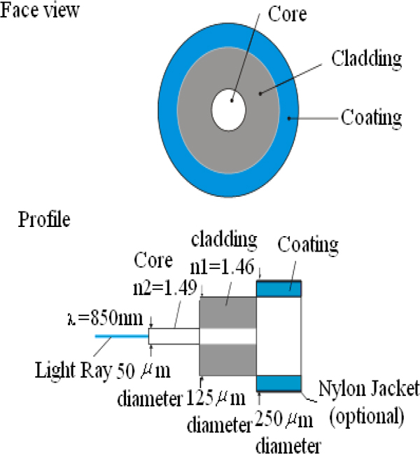
Fibre optic cable components
Fibre core
The core of the cable consists of a glass fibre through which the light signal travels. The most common core sizes are 50 and 62.5 micrometers (microns) for multimode cables and 8-10 microns for single mode cables.
Cladding
The core and cladding is manufactured as a single unit. The cladding is a protective layer with a lower refractive index than the core. The lower index means any light that hits the core walls will be redirected back to continue on its path. The cladding diameter is typically 125 microns.
Coating (buffer)
The coating is a protective layer around the cladding, and is typically a UV light-cured acrylate applied during the manufacturing process, for the physical and environmental protection of the fibre. Typical coating diameters are between 250 and 900 microns.
Strength members
Fibre optic cable also has strength members, which are strands of very tough material (such as steel, fibreglass, or Kevlar) that provide tensile strength for the cable. Each of these materials has advantages as well as drawbacks. For example, steel conducts electricity, making the cable vulnerable to lightning, but it will not disrupt an optical signal.
Cable sheath
The sheath of a fibre optic cable is an outer casing that provides primary mechanical protection, as with electrical cable. This is also referred to as a ‘jacket’.
16.3 Public network provided services
When the RTUs of a telemetry system are to lie outside the immediate boundaries of an industrial site, it is often necessary to lease the communications services of a public telephone network provider, to get reliable communications access to them. Quite often, this may be the only option as the sites may be too distant for line of sight radio or microwave or may be obstructed by mountains or buildings or there may be problems obtaining suitable frequencies in built up urban and industrial environments where the frequency spectrum is often very crowded.
The main providers of infrastructure and services are generally referred to as carriers. There are a number of smaller suppliers who buy large blocks of capacity from the main carriers and then resell smaller pieces of this capacity. These are mostly data services and are quite often only available in central business districts.
IDC recommend that once you have decided on the type of service you require, it is worth contacting the various carriers and suppliers to determine if they can provide this type of service to your master and RTU locations. Then a cost comparison should be carried out between the different service providers.
The telephone networks of the carriers are often referred to as the public switched telephone network or just the PSTN. The data networks are referred to as the public switched data network or PSDN.
The services provided by the smaller carriers and suppliers use fundamentally the same technology as those provided by the larger carriers. Quite often, the only difference between the services from different companies is the marketing name used for the service and the level of personal service and maintenance provided by the company.
16.4 Industrial Ethernet
Ethernet is the most popular lower-layer protocol used in LANs. Ethernet was first developed in 1972 at the Xerox Palo Alto research centre (PARC). This version of Ethernet supported a data transfer speed of 2.94Mbps. There have been several enhancements to the original version of Ethernet, and the current versions support network transmission speeds ranging from 10Mbps to 1,000Mbps. The 100Mbps speed is called as fast Ethernet, and 1000Mbps, called Gigabit Ethernet.
Ethernet uses a technique called the Carrier Sense Multiple Access/Collision Detection (CSMA/CD), also known as IEEE 802.3; to provide media access to devices on the network. Early Ethernet systems (of the 10 Mbps variety) use the CSMA/CD access method. This gives a system that operates with little delay if lightly loaded, but becomes very slow if heavily loaded. CSMA/CD is a probabilistic medium access mechanism, there is no guarantee of message transfer and messages cannot be prioritized.
Modern Ethernet systems are a far cry from the original design. From 100BASE-T onwards they are capable of full duplex (sending and receiving at the same time via switches, without collisions) and the Ethernet frame can be modified to make provision for prioritization and virtual LANs.
Ethernet is generally implemented as a 10 Mbps base band coaxial cable network. Carrier sense multiple access with collision detection (or CSMA/CD) is the media access control (or MAC) method used by Ethernet. This is the more popular approach with LANs.
The philosophy of Ethernet originated from radio transmission experiments with multiple stations endeavouring to communicate with each other at random times. Essentially before a station (or node) transmits a message (on the common connecting cable) to another node, it first listens for any bus (cable or radio) activity. If it detects that there are no other nodes transmitting, it sends its message. There is a probability that another station may attempt to transmit at precisely the same time. If there is a resultant collision between the two nodes, both nodes will then back off for a random time before reattempting to transmit (hopefully at different times because of the random delay). A typical view of the construction of the medium access control unit for each Ethernet station is given in Figure 16.2.
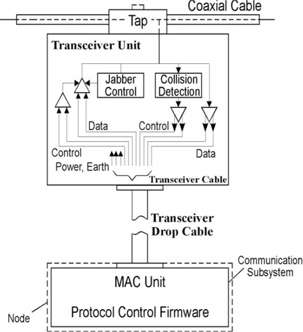
A typical hardware layout for a CSMA/CD system
The integrated tap and transceiver unit (referred to as the MAC unit) has the following components:
- A transceiver unit to transmit and receive data, detect collisions, provide electrical isolation and protect the bus from malfunctions
- A tap to make a non intrusive physical connection of the coaxial cable
The controller card, which is connected to the transceiver by shielded cable, contains a medium access control unit, which performs the framing of the messages and error detection, and a microprocessor for implementing the network dependent protocols. There are three types of Ethernet cabling, standard Ethernet, coaxial Ethernet or 10BASE2 and the 10BASE-T standard.
Standard Ethernet is referred to in the ISO 8802.3 standard as 10BASE5. This is understood to mean 10 Mb/sec giving base band transmission with a maximum segment length of 500 m (with each segment having up to 100 MAUs). There is a maximum of five segments allowed in the complete Ethernet system.
The 10BASE5 standard requires 50-ohm coaxial cable with 10.28 mm of that can be tapped using a clamp on tap. This is also referred to as thick wire Ethernet. Male N-connectors are used on the cable for splicing and a female–female N-type connector barrel between the two connectors. The attachment unit interface (AUI) is a 15 conductor shielded cable (consisting of five individually shielded pairs). Each end of a segment must be terminated with a 50 ohm N-connector terminator.
The medium attachment unit (or MAU) is available in two forms:
- A vampire tap
- The vampire tap allows easy connection to the coaxial cable as one pin is connected to the centre conductor (by drilling a hole into the cable) and the other pin is connected into the shield
- The N-type connector
- The N-type connector consists of two female N connectors thus requiring the cable be cut and male N-type connectors attached where the MAU is to be connected to the trunk line. In a dirty factory environment this approach is preferable to the vampire connection. The minimum connection distance between MAU is 2.5m
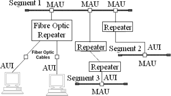
Physical layout for 10BASE5 Ethernet
Thin coaxial Ethernet or 10BASE2 were developed after the 10BASE5 standard and is designed to reduce the costs of installation. The maximum segment length is 185 m. Other names for 10BASE2 are cheaper net and thin wire Ethernet. The coaxial cable used is type RG-58 A/U or C/U with 50 ohm characteristic impedance. The trunk coaxial cable of thin Ethernet should not be spliced. Thin Ethernet MAUs may only be connected at consistent distance intervals of 0.5 m. On each 185 m segment of 10BASE2, up to 30 MAUs may be attached, including the MAUs for repeaters. Similar rules are followed as for installation of 10BASE5 except that a segment of thin coaxial cable may not be used as a link segment between two 10BASE5 segments.
A third Ethernet standard is 10BASE-T. This consists of a star type network with a central hub running twin twisted pair cable to each terminal. The maximum distance a terminal can be from the hub is 100 m. This is for servicing small collections of terminals and is usually tied back into a 10BASE5 network. A few suggestions on reducing collisions in an Ethernet network are:
- Keep all cables as short as possible
- Keep all high activity sources and their destinations as close as possible
- Possibly isolate these nodes from the main network backbone with bridges/routers to reduce backbone traffic
- Use buffered repeaters rather than bit repeaters
- Check for unnecessary broadcast packets which are aimed at nonexistent nodes
- Remember that the monitoring equipment to check out network traffic can contribute to the traffic (and the collision rate)
- Ensure that earthing of the cable is done at only one point on one of the cable terminators.
Fast Ethernet
Fast Ethernet provides a transmission speed of 100Mbps, ten times faster than that of “ordinary Ethernet”. It does however, retain the same frame format. It is described by two standards, namely IEEE 802.3u and IEE 802.3y.
IEEE 802.3u defines three different versions based on the physical media namely 100Base-TX (which uses two pairs of category 5UTP or STP), 100Base-T4 (which uses four pairs of wires of category 3,4 or 5UTP) and 100Base-FX (which uses multimode or single-mode fibre optic cable).
IEEE 802.3y, on the other hand, defines 100Base-T2 which uses two pairs of wires of category 3, 4, or 5 UTP.
Gigabit Ethernet
Gigabit Ethernet uses the same 802.3 frame format as 10 Mbps and 100 Mbps Ethernet systems. This operates at ten times the clock speed of fast Ethernet at 1 Gbps. By retaining the same frame format as the earlier versions of Ethernet, backward compatibility is assured with earlier versions, increasing its attractiveness by offering a high bandwidth connectivity system to the Ethernet family of devices.
Gigabit Ethernet is defined by the IEEE 802.3z standard. This defines the gigabit Ethernet media access control (MAC) layer functionality as well as three different physical layers: 1000Base-LX and 1000Base-SX using fibre and 1000Base-CX using copper. IBM originally developed these physical layers for the ANSI fibre channel systems and used 8B/10B encoding to reduce the bandwidth required to send high speed signals. The IEEE merged the fibre channel to the Ethernet MAC using a gigabit media independent interface (GMII) which defines an electrical interface enabling existing fibre channel PHY chips to be used and enabling future physical layers to be easily added. 1000Base-T is being developed to provide service over four pairs of category 5 or better copper cable. As discussed earlier this uses the same technology as 100Base-T2. This development is defined by the IEEE 802.3ab standard. These gigabit Ethernet versions are summarized in Figure 16.4.
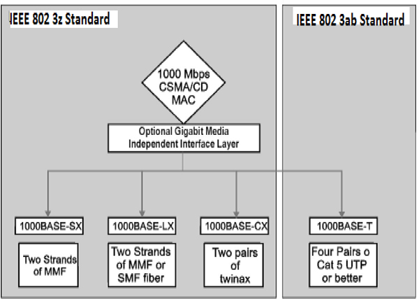
Gigabit Ethernet versions
16.5 TCP/IP
TCP/IP is the de facto global standard for the Internet (network) and host–to–host (transport) layer implementation of internetwork applications because of the popularity of the Internet. The Internet (known as ARPANet in its early years), was part of a military project commissioned by the Advanced Research Projects Agency (ARPA), later known as the Defense Advanced Research Agency or DARPA. The communications model used to construct the system is known as the ARPA model.
Whereas the OSI model was developed in Europe by the International Standards Organization (ISO), the ARPA model (also known as the DoD model) was developed in the USA by ARPA. Although they were developed by different bodies and at different points in time, both serve as models for a communications infrastructure and hence provide ‘abstractions’ of the same reality. The remarkable degree of similarity is therefore not surprising.
Whereas the OSI model has 7 layers, the ARPA model has 4 layers. The OSI layers map onto the ARPA model as follows.
- The OSI session, presentation and applications layers are contained in the ARPA process and application layer
- The OSI transport layer maps onto the ARPA host–to–host layer (sometimes referred to as the service layer)
- The OSI network layer maps onto the ARPA Internet layer
- The OSI physical and data link layers map onto the ARPA network interface layer.
The relationship between the two models is depicted in Figure 16.5.
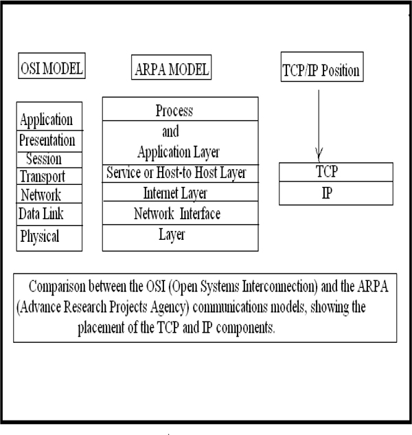
OSI vs. ARPA models
TCP/IP, or rather– the TCP/IP protocol suite– is not limited to the TCP and IP protocols, but consists of a multitude of interrelated protocols that occupy the upper three layers of the ARPA model. TCP/IP does NOT include the bottom network interface layer, but depends on it for access to the medium.
As depicted in Figure 16.6, an Internet transmission frame originating on a specific host (computer) would contain the local network (for example, Ethernet) header and trailer applicable to that host. As the message proceeds along the Internet, this header and trailer could be replaced depending on the type of network on which the packet finds itself– be that X.25, frame relay or ATM. The IP datagram itself would remain untouched, unless it has to be fragmented and reassembled along the way.
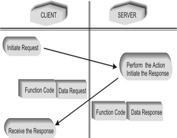
Internet frame
The Internet layer
This layer is primarily responsible for the routing of packets from one host to another. Each packet contains the address information needed for its routing through the internet work to the destination host. The dominant protocol at this level is the internet protocol (IP). There are, however, several other additional protocols required at this level such as:
- Address resolution protocol (ARP), RFC 826. This is used for the translation of an IP address to a hardware (MAC) address, such as required by Ethernet
- Reverse address resolution protocol (RARP), RFC 903. This is the complement of ARP and translates a hardware address to an IP address
- Internet control message protocol (ICMP), RFC 792. This is a protocol used for exchanging control or error messages between routers or hosts.
The host–to–host layer
This layer is primarily responsible for data integrity between the sender host and receiver host regardless of the path or distance used to convey the message. It has two protocols associated with it, namely:
- User data protocol (UDP), a connectionless (unreliable) protocol used for higher layer port addressing with minimal protocol overhead (RFC 768)
- Transmission control protocol (TCP), a connection–oriented protocol that offers a very reliable method of transferring a stream of data in byte format between applications (RFC 793).
The process/application layer
This layer provides the user or application programs with interfaces to the TCP/IP stack. These include (but are not limited to) file transfer protocol (FTP), trivial file transfer protocol (TFTP), simple mail transfer protocol (SMTP), telecommunications network (TELNET), post office protocol (POP3), remote procedure calls (RPC), remote login (RLOGIN), hypertext transfer protocol (HTTP) and network time protocol (NTP). Users can also develop their own application layer protocols.
16.6 Fieldbus
The two main Fieldbus standards that may impact on SCADA systems are discussed below. They are:
- Profibus
- Foundation Fieldbus
Profibus
ProfiBus (Process Field BUS) is a widely accepted international networking standard, commonly found in process control and in large assembly and material handling machines. It supports single-cable wiring of multi-input sensor blocks, pneumatic valves, complex intelligent devices, smaller sub-networks (such as AS-i), and operator interfaces.
ProfiBus is widely used in Europe and is also popular in North America, South America, and parts of Africa and Asia. It is an open, vendor independent standard. It adheres to the OSI model, ensuring that devices from a variety of different vendors can communicate easily and effectively. It has been standardized under the German National standard as DIN 19 245 Parts 1 and 2 and, in addition, has also been ratified under the European national standard EN 50170 Volume 2.
The development of ProfiBus was initiated by the BMFT (German Federal Ministry of Research and Technology) in cooperation with several automation manufacturers in 1989. The bus interfacing hardware is implemented on ASIC (Application Specific Integrated Circuit) chips produced by multiple vendors, and is based on RS-485 as well as the European EN50170 Electrical specification.
ProfiBus uses 9-Pin D-type connectors (impedance terminated) or 12mm round (M12-style) quick-disconnect connectors. The number of nodes is limited to 127. The distance supported is up to 24 km (with repeaters and fibre optic transmission), with speeds varying from 9600 bps to 12 Mbps. The message size can be up to 244 bytes of data per node per message (12 bytes of overhead for a maximum message length of 256 bytes), while the medium access control mechanisms are polling and token passing. ProfiBus supports two main types of devices, namely, masters and slaves.
- Master devices control the bus and when they have the right to access the bus, they may transfer messages without any remote request. These are referred to as active stations
- Slave devices are typically peripheral devices i.e. transmitters/sensors and actuators. They may only acknowledge received messages or, at the request of a master, transmit messages to that master. These are also referred to as passive stations.
There are several versions of the standard:
- ProfiBus DP (Distributed Peripheral) is intended for use at the plant floor level. It allows the use of multiple master devices, in which case each slave device is assigned to one master. Multiple masters can read inputs from the device but only one master can write outputs to that device. ProfiBus DP is designed for high speed data transfer at the sensor/actuator level, as opposed to ProfiBus FMS, which tends to focus on the higher automation levels. It is suitable as a replacement for the costly wiring of 24V and 4-20 mA measurement signals. The data exchange for ProfiBus DP is generally cyclic in nature. The central controller, which acts as the master, reads the input data from the slave and sends the output data back to the slave. The bus cycle time is much shorter than the program cycle time of the controller (less than 10 mS)
- ProfiBus FMS (Fieldbus Message Specification) is a peer to peer messaging format, which allows masters to communicate with one another. Just as in ProfiBus DP, up to 126 nodes are available and all can be masters if desired. FMS messages consume more overhead than DP messages. Profibus FMS is used for interconnecting DCSs, PLCs, etc.
- ‘COMBI mode’ is when FMS and DP are used simultaneously in the same network, and some devices (such as Synergetic’s DP/FMS masters) support this. This is most commonly used in situations where a PLC is being used in conjunction with a PC, and the primary master communicates with the secondary master via FMS. DP messages are sent via the same network to I/O devices.
- Profibus PA: Profibus DP is aimed at the automation industry (motor control etc). Its application in a process control environment, however, requires an intrinsically safe (explosion proof) option and this is the reason for Profibus PA. The ProfiBus PA protocol is the same as for ProfiBus DP, except that voltage and current levels are reduced to meet the requirements of intrinsic safety (class I division II) for the process industry. Many DP/FMS master cards support ProfiBus PA, but barriers are required to convert between DP and PA. The initial implementation of PA used the transmission technique specified in IEC 61158-2 (which Foundation Fieldbus H1 uses as well). IEC-61158 is, however, very slow and this has led to the introduction of RS-485 IS, an intrinsically safe version of RS-485.
Foundation Fieldbus
Foundation Fieldbus allows end-user benefits such as:
- Reduced wiring
- Communications of multiple process variables from a single instrument
- Advanced diagnostics
- Interoperability between devices of different manufacturers
- Enhanced field level control
- Reduced start-up time
- Simpler integration.
The concept behind Foundation Fieldbus is to preserve the desirable features of the present 4-20 mA standard (such as a standardized interface to the communications link, bus power derived from the link and intrinsic safety options) while taking advantage of the new digital technologies. This provides the features noted above because of:
- Reduced wiring due to the multi-drop capability
- Flexibility of supplier choices due to interoperability
- Reduced control room equipment due to distribution of control functions to the device level
- Increased data integrity and reliability due to the application of digital communications.
Foundation Fieldbus implements four OSI layers. Three of them correspond to OSI layers 1, 2 and 7. The fourth is the ‘user layer’ that sits in top of layer 7 and is often said to represent OSI ‘layer 8’.The user layer provides a standardized interface between the application software and the actual field devices.
16.7 Modbus
The Modbus Messaging Protocol is an application layer (OSI layer 7) protocol that provides communication between devices connected to different types of buses or networks. It implements a client/server architecture that operates essentially in a “request/response” mode, irrespective of the Media Access Control method used at layer 2. The client (on the controller) issues a request; the server (on the target device) then performs the required action and initiates a response.
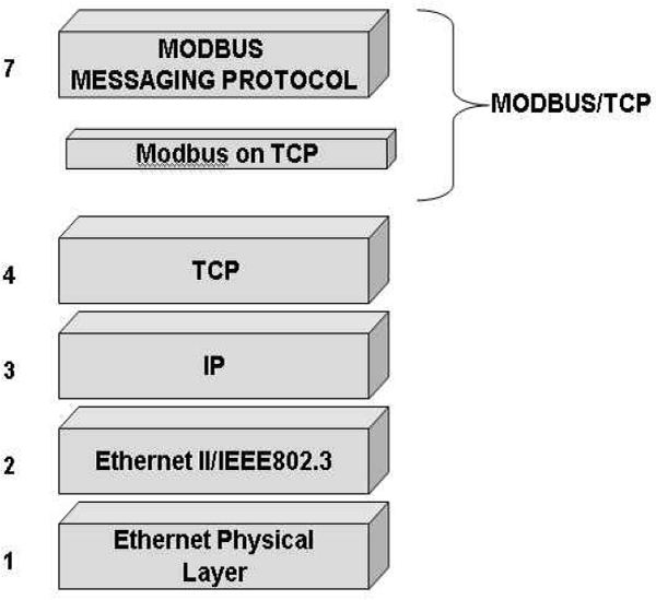
Modbus transaction
In order to match the Modbus Messaging protocol to TCP, an additional sub-layer is required. The function of this sub-layer is to encapsulate the Modbus Protocol Data Unit (PDU) in such a way that it can be transported as a packet of data by TCP/IP.
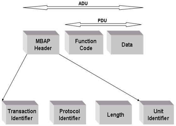
Modbus/TCP communication stack
Modbus encapsulation
Those familiar with the TCP/IP protocol suite might wonder why connection-oriented TCP is used rather than the datagram-oriented User Datagram Protocol (UDP). TCP has more overheads, and consequently it is slower than UDP. The main reason for this choice is to keep control of individual “transactions” by enclosing them in connections that can be identified, supervised, and cancelled without requiring specific action on the part of the client or server applications. This gives the mechanism a wide tolerance to network performance changes, and allows security features such as firewalls and proxies to be introduced.
The PDU consisting of Data and Function Code is encapsulated by adding a “Modbus on TCP Application Protocol” (MBAP) header in front of the PDU. The resulting Modbus/TCP ADU (Application Data Unit), consisting of the PDU plus MBAP header, is then transported as a chunk of data via TCP/IP and Ethernet.
Whereas Modbus Serial forms the ADU by simply appending a one-byte Unit Identifier to the PDU, the MBAP header is much larger, although it still contains the Unit Identifier for communicating with serial devices. A byte count is included so that in the case of long messages being split up by TCP, the recipient is kept informed of the exact number of bytes transmitted. Note that the ADU no longer contains a checksum as this function is performed by TCP.
| Fields | Length | Description | Client | Server |
|---|---|---|---|---|
| Transaction identifier | 2 bytes | Identification of a Modbus request/response transaction | Initialized by the client | Copied by the server from the required request |
| Protocol identifier | 2 bytes | 0 = Modbus protocol | Initialized by the client | Copied by the server from the received request |
| Length | 2 bytes | Number of following bytes | Initialized by the client | Initialized by the server (response) |
| Unit identifier | 1 byte | Identification of a remote device (slave) connected on a serial line or on other buses | Initialized by the client | Copied by the server from the received request |
The MBAP header is 7 bytes long and comprises the following four fields:
- The Transaction Identifier is a pseudo-random number used for pairing requests and responses. The Modbus server does not interpret this, but simply copies this number received in the request from the client back into the response to the client. The client normally generates this number by means of a counter.
- The Protocol Identifier is used for multiplexing between systems. The Modbus protocol is defined as value 0 (0 × 00).
- The Length field is a byte count of all the fields following it, including the Unit Identifier and data fields.
- The Unit Identifier is used for routing between systems, typically to a Modbus Serial or Modbus Plus target device through a gateway between the serial line and the TCP/IP network. The client sets it and the server must return the same value.
The Modbus/TCP ADU is therefore constructed as follows:
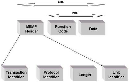
Modbus/TCP ADU
All Modbus/TCP ADUs are sent via a well-known port (502) and the fields are encoded big-endian, which means that if a number is represented by more than one byte, the most significant byte is sent first. TCP/IP transports the entire Modbus ADU as data. This is shown in the following figure.
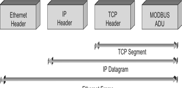
Transportation of Modbus ADU
Modbus component architecture model
The following figure shows a system with both client and server devices, that is controllers and target devices.
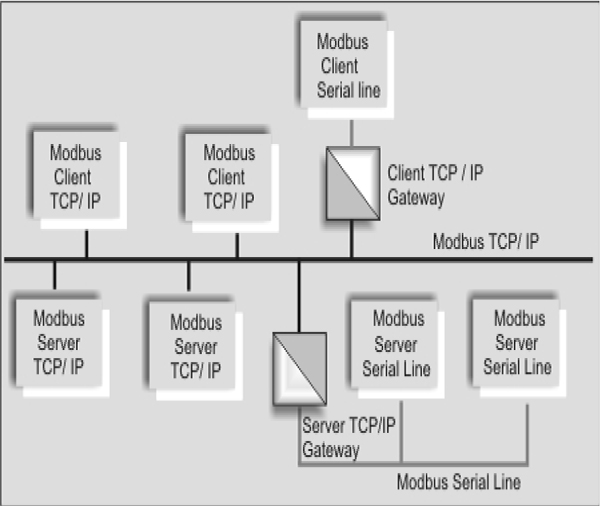
Modbus gateways
Some are connected via Ethernet, while others are serial (RS-232 or RS-485) devices connected to the Ethernet network via Modbus gateways. The gateways are Modbus Serial to Modbus/TCP converters, as produced by several vendors.
Each of the TCP/IP-enabled devices in the above figure supports the Modbus Messaging Service architecture. The following is a graphical representation of this architecture and the way it relates to the TCP/IP stack. The communication application layer corresponds to Layer 7 of the OSI model, while the TCP/IP stack corresponds to OSI layers 3 and 4. The TCP management layer acts as an interface between the two.
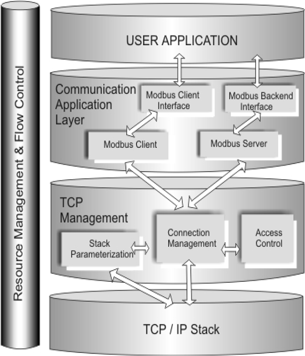
Modbus messaging service architecture
A Modbus device can be a client device or a server device and as such it can provide a client and/or a server interface to the user application. The server interface is called a “backend interface” as it allows indirect access to user application objects such as discrete inputs, coils, input registers, and holding registers.
The application program on the client device sends explicit instructions to a remote server device by exchanging control information with the Modbus client. The Modbus client, in turn, builds a Modbus request with parameters obtained from the application program and passes this message on to the server. The processing of this request involves waiting for a reply and the generation of a Modbus confirmation.
The Modbus client interface allows the application to exchange information with the Modbus client through an Applications Programming Interface (API). The Modbus server maintains a constant listening watch on port 502. When it receives a request from the client, it actions the appropriate read, write, or any other function to the application program via the backend interface. It then returns the appropriate response to the client.
In order to control the equilibrium in the flow of inbound and outbound messages, flow control is implemented at various levels. It is primarily based on TCP flow control, with some additional control at the Data Link and application layers.
Modbus/TCP operation
Communication between a Modbus client and Modbus server requires a TCP connection. The user application software can establish this connection explicitly or it can be taken care of automatically by the TCP connection management module. The number of concurrent TCP connections is not dictated by the Modbus specification, but is dependent on the capabilities of the device. The following implementation rules are also prescribed by the specification:
- The TCP connection should be kept open and not closed and re-opened for every transaction
- The number of concurrent connections between a client and a server should be kept to a minimum
- Several Modbus transactions can be activated on the same TCP connection, albeit with different transaction identifiers
- For a bidirectional client/server link, a TCP connection needs to be established in each direction a TCP frame may only carry one Modbus ADU
In order to establish a connection, a client and a server must negotiate a TCP connection with a registered port number bigger than 1023 on the client and the well-known port number 502 on the server. On the server side, only port 502 is used, but on the client side each subsequent connection will require a different port number.
Once the connection is established, the client and server will exchange requests and responses. This will continue until the client is done, at which point it will attempt to close the connection with a FIN. The server may respond in kind or simply acknowledge with an ACK, because it is not ready to close the connection yet, resulting in a half-close. When the server is ready to close as well, it will issue a FIN to which the client will respond with an ACK.
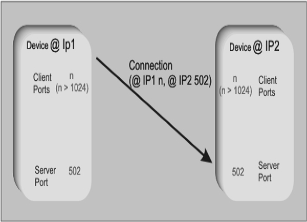
Modbus TCP connection establishment
The connection is then closed (see the following figure). Only one Modbus transaction is shown here, but there could be many within the one TCP connection.
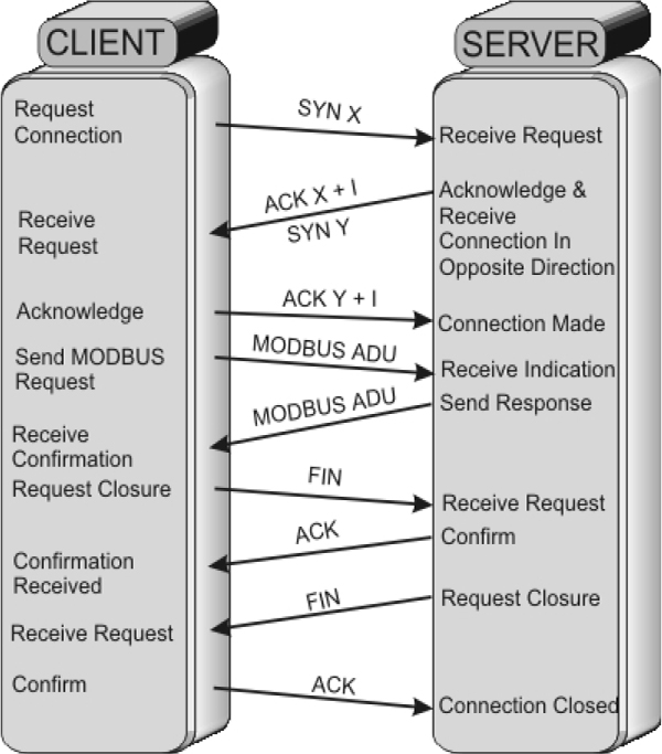
Client–server interaction
Troubleshooting
Troubleshooting Modbus TCP is extremely easy, provided the troubleshooting understands Ethernet as well as TCP/IP and Modbus Serial.
The Modbus/TCP frames can be captured and displayed by means of a protocol analyser such as Wireshark. This will break down the Modbus/TCP ADU down to byte level. The only new factor introduced here is the MBAP header.
If a Modbus/TCP to Modbus Serial gateway does not work despite being set up properly, connect a Modbus master simulator on the Ethernet side and a Modbus slave simulator on the serial side. Then generate simple requests such as “Read coils.” Monitor the packets (requests as well as responses) on both sides and look for corrupted fields in the packets. For example, if the Transaction Identifier (in the MBAP header) for the request and response messages is not the same, the master will reject the slave response.
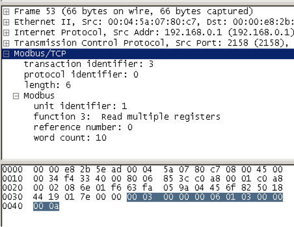
Modbus/TCP transaction on protocol analyser
16.8 LAN connectivity
Distances of LANs are often limited and there is often a need to increase this range. There is a number of interconnecting devices, which can be used to achieve this ranging from repeaters to routers to gateways. It may also be necessary to partition an existing network into separate networks for reasons of security or traffic overload.
These components to be discussed separately are
- Bridges
- Routers
- Switches
Bridges
Bridges are used to connect two separate networks to form a logical network. The bridge has a node on each network and passes only valid messages across to destination addresses on the other network(s). The bridge stores the frame from one network and examines its destination address to determine whether it should be forwarded over the bridge. Figure 16.16 shows the basic configuration of an Ethernet Bridge.
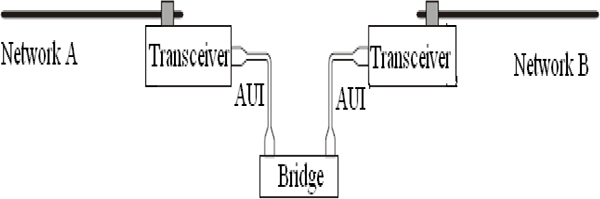
Ethernet Bridge
The bridge maintains records of the Ethernet addresses of the nodes on both networks to which it is connected. The data link protocol must be identical on both sides of the bridge; however, the physical layers (or cable media) do not necessarily have to be the same. Thus, the bridge isolates the media access mechanisms of the networks. Data can therefore be transferred between Ethernet and token ring LANs. For example, collisions on the Ethernet system do not cross the bridge nor do the tokens. The bridge provides a transparent connection between a full size LAN with maximum count of stations, repeaters and cable lengths and any other LAN.
Bridges can be used to extend the length of a network (as with repeaters) but in addition, they improve network performance. For example, if a network is demonstrating slow response times, the nodes that mainly communicate with each other can be grouped together on one segment and the remaining nodes can be grouped together in another segment. The busy segment may not see much improvement in response rates (as it is already quite busy) but the lower activity segment may see quite an improvement in response times. Bridges should be designed so that 80% or more of the traffic is within the LAN and only 20% crosses the bridge. Stations generating excessive traffic should be identified by a protocol analyser and relocated to another LAN.
Routers
Routers are used to transfer data between two networks that have the same network layer protocols (such as TCP/IP) but not necessarily the same physical or data link protocols. Figure 16.17 shows the application of routers.
The routers maintain tables of the networks to which they are attached and to which they can route messages. Routers use the network (IP) address to determine where the message should be sent, because the network address contains routing information.
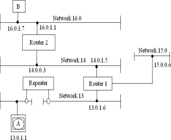
Router applications
Routers maintain tables of the optimum path to reach particular network and redirect the message to the next router along that path. For example in Figure 16.17, to transmit a message from node A on network 13.0 to node B on network 16.0, router 1 forwards the message onto network 14.0 and router 2 forwards it to network 16.0.
Router 1 stores the message from A and examines the IP address of the destination (16.0.1.7). Consulting its routing table it determines that the message needs to be sent to router 2 in order to reach network 16.0. It then replaces the destination hardware address on the message with router 2’s address and forwards the message on network 14.0.
Router 2 repeats the process and determines from the destination IP address (16.0.1.7) that it can deliver the message directly on network 16.0. Router 2 establishes the hardware address (16.0.1.7) from its routing table and places that destination address on the message which it delivers on network 16.0.
Switches
One of the devices that has made a major change to the way networks and Ethernet are used today is the ubiquitous switch. This enables direct communications between multiple pairs of devices in full duplex mode; thus eliminating the limitations imposed by the classical Ethernet architecture.
Switches enable specific and discrete data transfers to be accomplished between any pair of devices on a network, in a dedicated fashion. Stemming from the STAR network, where each terminal had its own discrete cable to a central hub, it became apparent that there was a requirement for a network to be able to quickly and effectively connect 2 terminals or nodes together. This is to be done in such a manner that they had, in the case of Ethernet 10baseT a direct and dedicated 10 Mbps connection.
Illustrated below is an example of a Cisco Kalpana 8 port switch, with 8 Ethernet terminals attached. This comprises a star configuration, but it operates in a different manner.
Nodes or terminals 1 & 7, 3 & 5 and 4 & 8 are connected directly. For example, terminal 7, detecting CSMA/CD on its local connection sends a packet to the switch. The switch determines the destination address and directs the package to the corresponding port; Port 1 in this example. Data is then passed at 10 Mbps between the two devices.
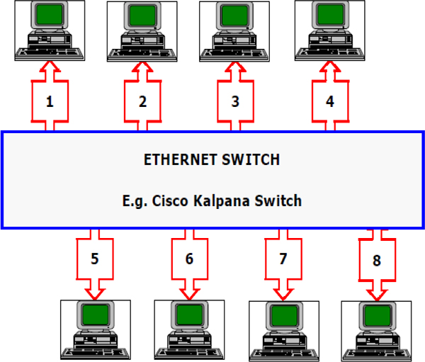
Ethernet switch
If terminal 3 wishes to communicate with terminal 5, the same procedure is initiated by device 3 as it was for terminal 7 as described above. In fact, if the switch was say a 16 port switch (an 8 port being shown in this example) it would be possible for 8 pairs of terminals to be simultaneously communicating between themselves, all at the Ethernet rate of 10 Mbps for each established circuit.
The switch must be able to detect, from the packet header, the Ethernet destination address, and effect the required port connection in time for the remainder of the packet to be switched through. Some switches cannot achieve this requirement; their switching is slower than the effective requirement made on them by the transmission speeds. These switches are known as store-and-forward switches, and delay the packet by the time required to store, switch and forward it.

Full duplex switch between a terminal and a file server
An additional advancement is full duplex Ethernet where a device can simultaneously transmit and receive data over one Ethernet connection. This requires a different Ethernet card, supporting the 802.3x protocol, to a terminal, and utilizes a switch; the communication becomes full duplex. The node automatically negotiates with the switch and uses full duplex if both devices can support it.
This form of configuration is useful in places where large amounts of data require to be moved around quickly. For example, graphical workstations, large colour plotters and fileservers.
16.9 SCADA Network Security
Ideally, a SCADA or process control network would be a closed system, accessible only by trusted internal components such as the Human Machine Interface (HMI) stations and data historians. Many systems now utilise local and wide area networks (LANs and WANs) to provide data connectivity between SCADA system servers and their local controllers such as PLCs, RTUs and IEDs etc as well as for communications across organizations. These technologies provide many benefits, but bring with them the threat of unauthorised access to critical control system architecture. The threat is greatly magnified if common shared communication systems such as the Internet are incorporated in the SCADA systems. Therefore the implementation of effective network security systems is essential to minimise these risks.
Realistically, there is a need to provide for external access to parts of all SCADA systems from both corporate users and selected Third-parties. For example, production and maintenance management information needs to be relayed to computers and users outside of the plant floor for management purposes, while vendors may need to be given access to controllers for support purposes. This means that some network paths need to be provided from the outside, untrusted world to internal control components.
The goal of the network security system components, such as firewalls, is to provide such external access while minimizing the risk of unauthorized access (or network traffic) to internal components on the SCADA systems. Such a risk minimization strategy will typically include the following general objectives:
- No direct connections from the Internet to the SCADA network and vice-versa
- Restricted access from the enterprise network to the control network
- Unrestricted (but only authorized) access from the enterprise network to shared PCN/enterprise servers
- Secure methods for authorized remote support of control systems
- Secure connectivity for wireless devices (if used)
- Well-defined rules outlining the type of traffic permitted on a network
- Monitoring of traffic attempting to enter and on the network
- Secure connectivity for management of the firewall.
Cryptography primer
Cryptography moderates the risk posed by the insecurities. The media used for data transfer is insecure and need to be authorized as unauthorized individuals may access the medium and interrupt messages exchanged between lawful system users. They may also inject data of their own in an attempt to gain information or access to devices to which they are not entitled.
Modern cryptography consists of functions and algorithms operating on data to provide the necessary security. Cryptographic functions provide data privacy.
Encryption
Data Confidentiality: Two parties should be able to send private messages over an insecure medium without exposing the contents of the messages to attackers.
Encryption is the process of transforming a digital message from its original form into a form that cannot be interpreted by an “unauthorized” individual. The output of the coding process is a function of the message and code key. This encryption process must be completely reversible by an “authorized” individual with access to the secret decode key. Authority to read a message is only granted by sharing knowledge of the secret decryption key.
Learning objectives
- Understanding diagram layouts and formats
- Cross references
- P & IDs fundamentals
17.1 Understanding diagram layouts and formats
The instrument location drawing is used to indicate an approximate location of the instruments and junction boxes. This drawing is then used to determine the cable lengths from the instrument to the junction box or control room. This drawing is also used to give the installation contractor an idea as to where the instrument should be installed.
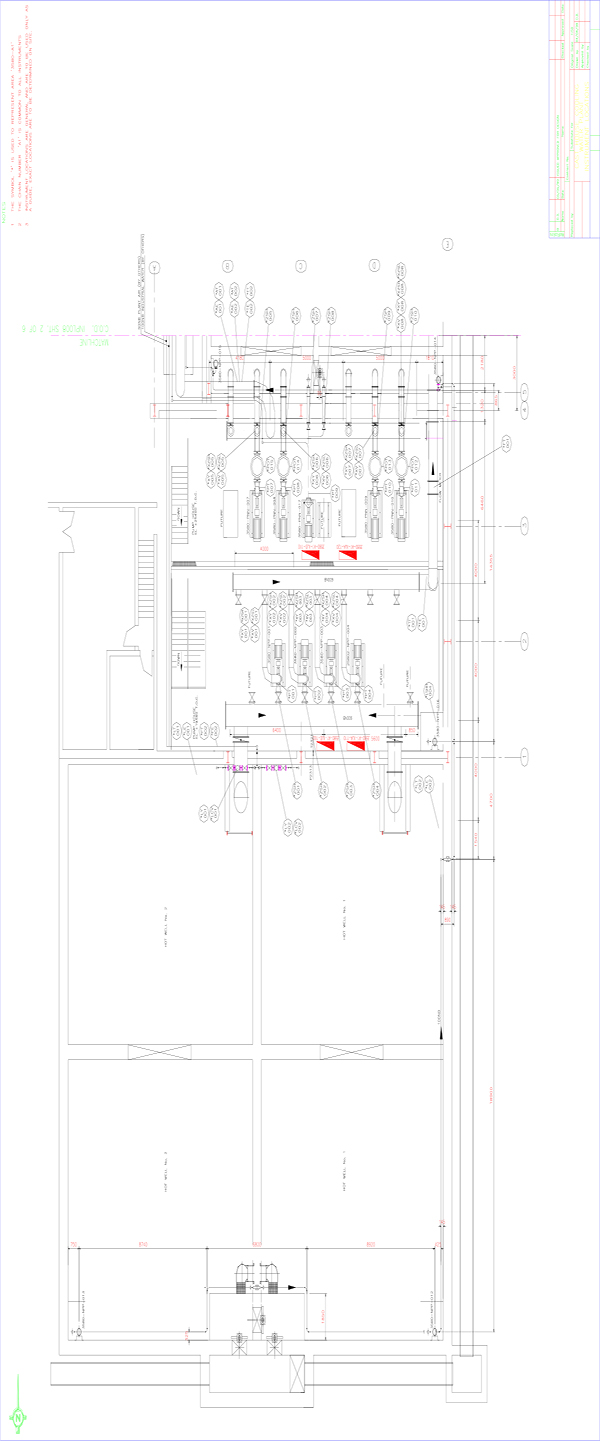
Instrument location plan
Instrument location plan (2)
The detail shows how the location drawing guides the installation contractor in the placement of the field junction boxes and the field instrumentation. It must be remembered that this is only a guide. This drawing is created using experience and imagination, the installation contractor deals with the physical aspects and may find excellent reasons for changing the design.
17.1.1 Cable racking layout
Use of the racking layout drawing has grown with use of 3D cad packages; this drawing shows the physical layout and sizes of the rack as it moves through the plant.
Cable racking layout
17.1.2 Cable routing layout
Prior to the advent of 3D cad packages, the routing layout used a single line to indicate the rack direction as well as routing and sizes and was known as a ‘Racking & Routing layout’.
Cable routing layout
17.1.3 Block diagrams – signal, cable and power block diagrams
Cable block diagrams can be divided into two categories: Power and Signal block diagrams. The block diagram is used to give an overall graphical representation of the cabling philosophy for the plant.
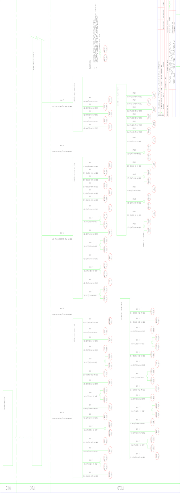
Block diagram
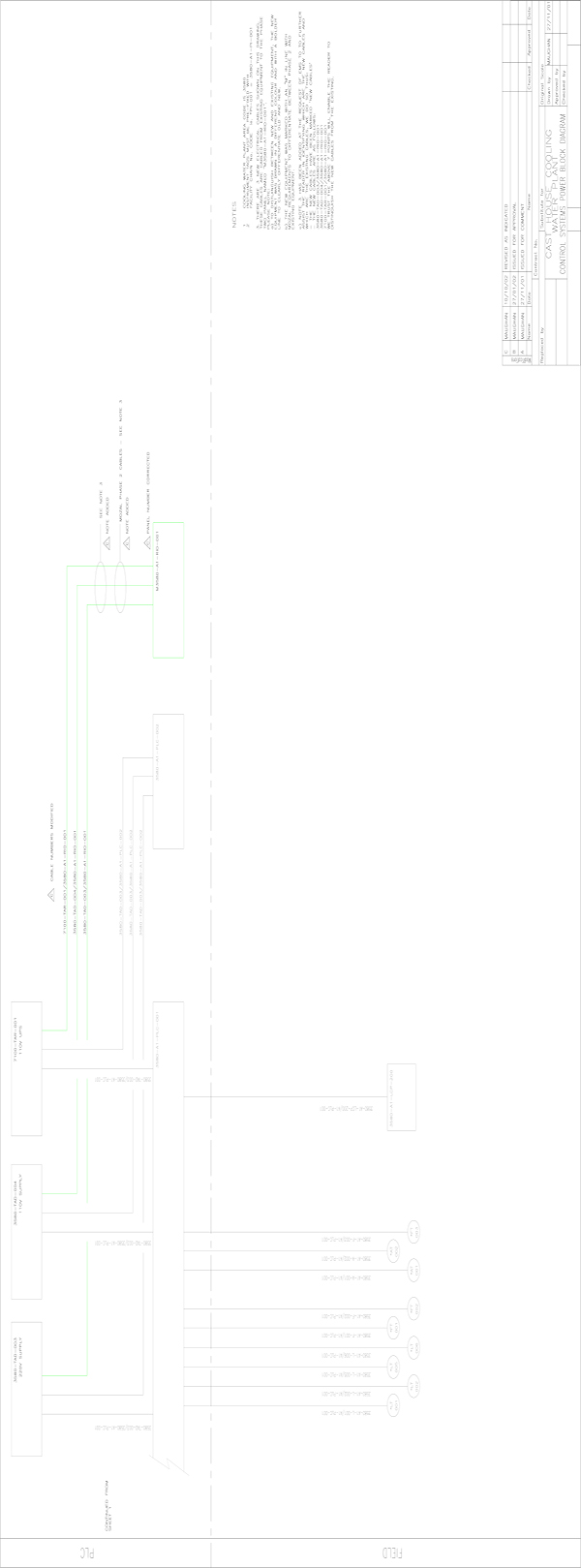
Block diagram (2)
17.1.4 Field connections/Wiring diagrams
Function: To instruct the wireman on how to wire the field cables at the junction box
Used by: Installation contractor, when the cable is installed on the cable rack, it is left lying loose at both the instrument and junction box ends. The installation contractor now stands at the junction box and strips each cable and wires it into the box according to the drawing.
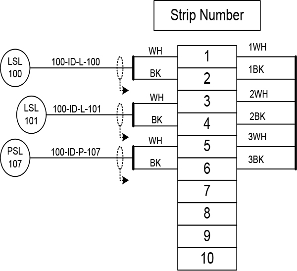
Field connections
17.1.5 Power distribution diagram
Function: There are various methods of supplying power to field instruments; the various formats of the power distribution diagrams show these different wiring systems. The diagrams below show the various options in greater detail. Note the difference between this diagram and the power block diagram
Used by: Various people depending on the wiring philosophy, such as the panel wireman, field wiring contractor.
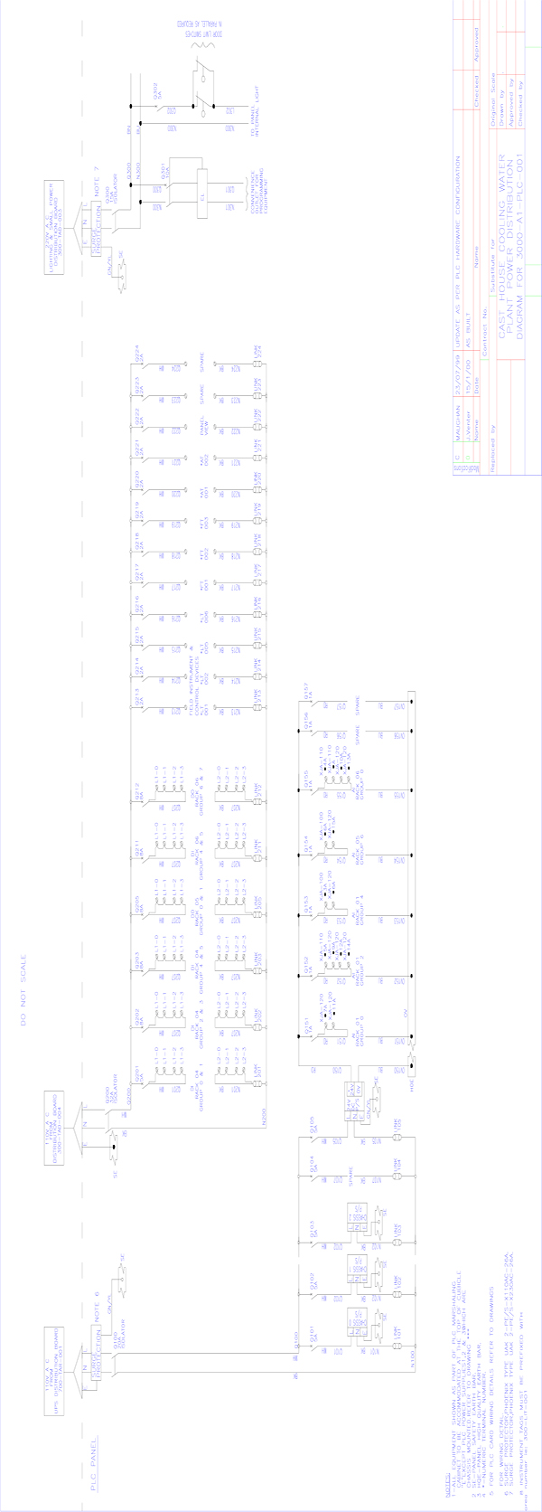
Power distribution diagram
17.1.6 Earthing diagram
Function: Used to indicate how the earthing should be done. Although this is often undertaken by the electrical discipline there are occasions when the instrument designer may or must generate his own scheme – e.g. for earthing of zener barriers in a hazardous area environment.
Used by: Earthing contractor for the installation of the earthing. This drawing should also be kept for future modifications and reference.
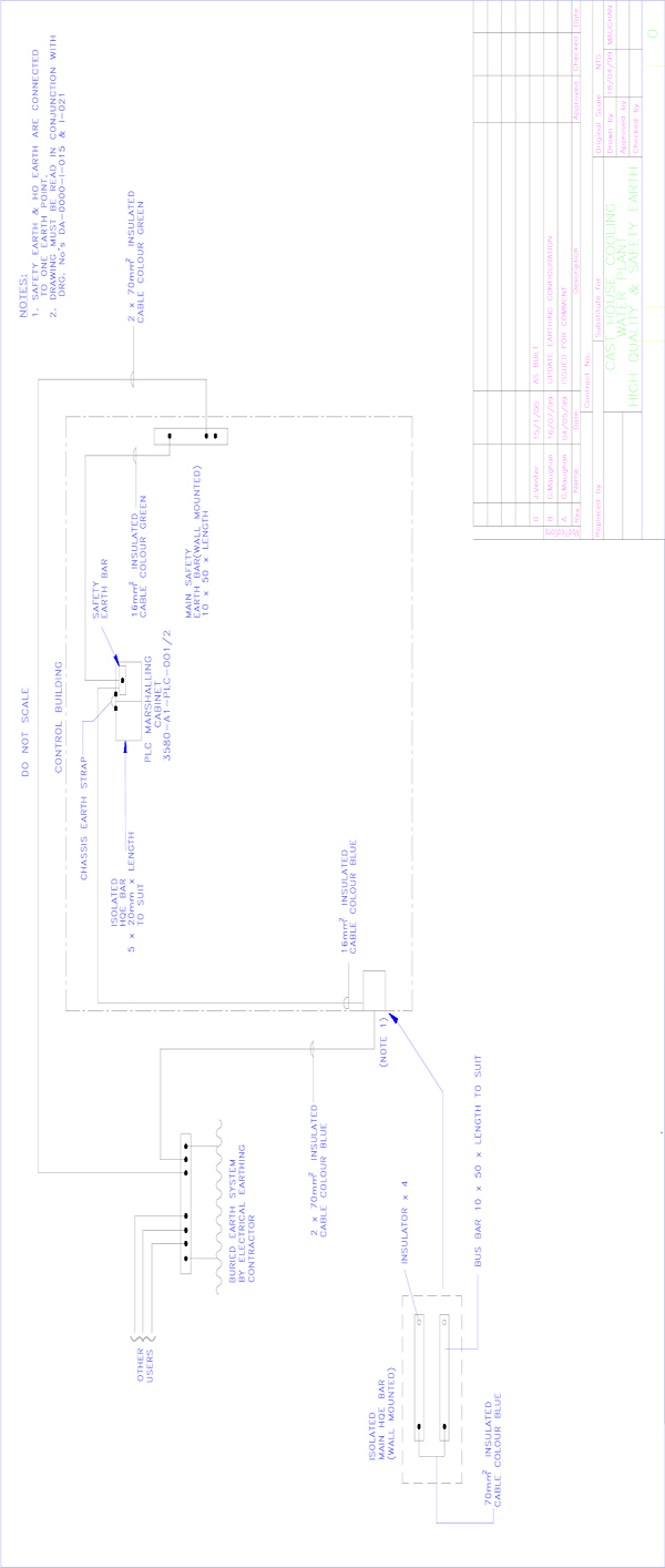
Earthing diagram
17.1.7 Loop diagrams
Function: A diagram that comprehensively details the wiring of the loop, showing every connection from field to instrument or I/O point of a DCS/PLC. The inclusion of a bubble diagram in the bottom left hand corner of the diagram quickly conveys to the reader the overall loop strategy.
Used by: Maintenance staff during the operation of the plant and by commissioning staff at start up.
Loop diagram
Loop diagram (2)
Loop diagram (3)
Loop diagram (4)
17.1.8 PLC schematics
PLC schematics give an overview the interaction of the field device (and associated wiring) with the I/O of a PLC or DCS system.
PLC schematics
17.1.9 Installation detail – hook-up
Function: To detail how the instrument should be installed by the instrument fitter. Used to list the components required for the installation.
Used by: Instrument fitter to install instrument, estimator to total equipment for purchase.
Installation details
17.1.10 Other diagrams
Depending on the particular plant a range of other drawings, lists, schedules etc may be required to full document the instrumentation on a plant.
Typical of these may be one or more of the following:
- Control Panel General Arrangement Drawings
- Ladder Logic Drawings
- Hazardous Area Drawings
- Installation Specification document
There are no specific standards covering the presentation of these documents and individual projects may differ in presentation although the information they communicate must be concise. An example of a simple general arrangement drawing for a SCADA system is shown.
SCADA installation
17.2 Cross references
Cross references – indicating where on the diagram or sequential sheet, the related parts of the equipment can be found. All associated contacts and coils are to be cross referenced using the format detailed in this section.
Cross referencing uses a XY reference system. The first two or three characters represent the sheet number and the last two or three characters represent the XY co-ordinates of the contact or coil etc. The cross reference will be distinguished from the wire numbers by placing the number in brackets. For example a contact which is on sheet 3 which has a XY co-ordinate of F12 shall be detailed on the associated coil as (03F12).
If wire numbers are cross referenced to other drawings the cross reference will contain the whole drawing number followed by the XY reference.
17.3 Piping and instrumentation diagrams (P&ID)
The Piping & Instrumentation Diagram, which may also be referred to as the Process & Instrumentation Diagram, gives a graphical representation of the process including hardware (Piping, Equipment) and software (Control systems); this information is used for the design construction and operation of the facility.
Other synonyms for the P&ID are:
- MFD – Mechanical Flow Diagram: Used where materials handling is predominant
- EFD – Engineering Flow Diagram
- UFD – Utility Flow Diagram
The PFD defines “The flow of the process” The PFD covers batching, quantities, output, and composition.
The P&ID also provides important information needed by the constructor and manufacturer to develop the other construction input documents (the isometric drawings, or orthographic physical layout drawings, etc.). The P&ID provides direct input to the field for the physical design and installation of field-run piping. For clarity, it is usual to use the same general layout of flow paths on the P&ID as used in the flow diagram.
The P&ID ties together the system description, the flow diagram, the electrical control schematic, and the control logic diagram. It accomplishes this by showing ALL of the piping, equipment, principal instruments, instrument loops, and control interlocks. The P&ID contains a minimum amount if text in the form of notes (the system description minimizes the need for text on the P&ID). The first P&ID in the set for the job should contain a legend defining all symbols used; if some symbols are defined elsewhere, it may be appropriate only to reference their source. The P&ID is also used by the start-up organizations for preparing flushing, testing, and blow-out procedures for the piping system and by the plant operators to operate the system. The correctness and completeness of the P&ID drawings are critical to the success of a plant start-up program.
There are several other facts concerning P&IDs that are important. First, regardless of how sophisticated the Design P&ID may be, there is a wealth of information that exists, and is needed by the typical operating plant, that does not exist during the initial design phase of the facility; and this information continues to grow throughout the plant’s operating life.
Because many plants serve 20 years or more, maintenance personnel need effective tools for corrective (repair) and preventive maintenance. During corrective maintenance, Intelligent P&IDs can assist the operator in finding information needed foe personnel assignment and location of spare parts. Engineering documents assist maintenance personnel by defining what is broken and determining how to replace it. The P&ID is the index to this data, providing quick access to the information and a tool to update and track that information after changes are made.
The operation phase concerns issues of safety as well as the process itself. The operator needs to keep a history of the processes, as well as the updates and changes to the plant data model. Intelligent P&IDs facilitate compliance with legislation such as OSHA and ISO, requiring that the P&ID and instrument data sheets are kept up-to-date and accessible.
Also, in today’s marketplace, the majority of projects are existing plants; either through re-work, upgrade, modernization program etc.
P&IDs for these facilities that are either purely paper-based, or only based on generic (dumb graphics) CAD systems, most likely AutoCAD or MicroStation.
Additionally, there exists a massive amount of legacy data in these plants, concerning all phases of the plant operations environment. Capturing this information and linking it to the existing P&ID, or even better, linking it to newly created Intelligent Design P&IDs, would provide an extremely valuable tool to the typical plant operator.
The typical plant operations environment uses the P&ID as the principal document to locate information about the facility, whether this is physical data about an object, or information, such as financial, regulatory compliance, safety, HAZOP information, etc.
The P&ID defines “The control of the flow of the process” Where the PFD is the main circuit, the P&ID is the control circuit.
Once thoroughly conversant with the PFD & Process description, the engineers from the relevant disciplines (piping, electrical & control systems) attend a number of HAZOP sessions to develop the P&ID.
HAZOP
Hazard operability studies have a full set of rules and procedures, which are beyond the scope of this course. In its most basic form, the HAZOP looks at each item of equipment in the process and by applying a given set of rules to each item determines suitability and possible problems. It is the resolution of these problems that leads to the development of the P&ID.
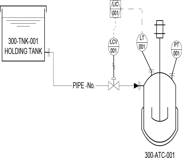
Coffee bottling plant
Returning to our coffee bottling plant as shown in figure 17.17, we see that if the holding tank runs dry while we are trying to fill the autoclave, the system will come to a standstill. We can resolve this problem by installing a level low switch on the holding tank; the level switch can then give an alarm when the tank level drops below a predetermined point.
Comparing figure 3.4 above to the PFD in figure 3.2, two things become immediately apparent:
- The level of detail in the P&ID is far greater than that of the PFD, focus has moved from the operation as a whole and now focuses, in great detail, on the operation of each piece of equipment.
- Showing this level of detail takes a great deal of space and includes far more lines on the drawing, for this reason rules are laid down detailing the amount of equipment to be shown per P&ID.
17.3.1 P&ID standards
Before development of the P&ID can begin a thorough set of standards is required, these standards must define the format of each component of the P&ID. The following should be shown on the P&ID:
- Mechanical Equipment
- Equipment Numbering
- Presentation on the P&ID
- Valves
- Hand valves
- Control valves
- Piping
- Pipe numbering
- Nozzles & Flanges
- Equipment & instrument numbering systems
A completed P&ID may therefore appear as shown in Figure 17.18.
Refer to Appendix A – Symbols and Numbering for more details.
Completed P & ID
Mechanical equipment
Mechanical equipment is shown in an outline form and indicates all associated equipment that is pertinent to the function of the equipment. For a vessel this would include any; trays, spray nozzles, demisters, packed sections etc.
Samples:
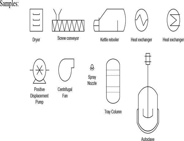
Mechanical Equipment
Equipment numbering
Equipment numbering varies from installation to installation. The equipment numbering system for a particular plant should be defined in the relevant equipment numbering specification.
Presentation on the P&ID
There are 3 common formats for presentation. Again, the accepted format should be defined in a standard – either a company, national or international standard.

Formats for Presentation
Valves
Valves fall into two main categories, control valves and hand valves. The control systems engineer specifies the control valve, while the hand valve is usually selected by the piping discipline.
Hand valves
Hand valves are denoted using the relevant symbol; a clear symbol is used to represent a normally open valve while an opaque symbol is used for normally closed valves. A solitary valve symbol is assumed to be a hand valve, as a control valve would show the control configuration and may be accompanied by an instrument “bubble”.
Hand Valves
Again, the manner in which the hand valve is displayed is dependant on the standard used by the originator of the P&ID.
Control valves
Control valves use the same basic valve type symbol as the hand valve, the following differences differentiate hand valve from control valves.
- Control valves do not use clear and opaque symbols to show standard positions
- Control valves show a failure position in the event of a power loss, these positions are Fail open (FO) , Fail Closed (FC) or Fail Indeterminate (FI) used when the valve will remain at the same position it was when the power was lost
- Control valves display the type of control i.e. actuator, diaphragm, solenoid etc
- Control valves should appear in the instrument list
Examples:
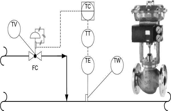
Globe control valve
The example in figure 17.22 shows a globe control valve with a pneumatic diaphragm actuator and an electro-pneumatic positioner together with a temperature element (TE) in a thermo well (TW) connected to a temperature transmitter (TT). This level of detail is not normally required on a P&ID and is often simplified to that shown in figure17.23.
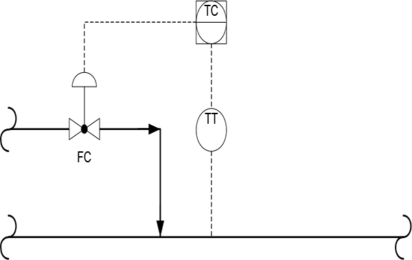
Simplified Globe control valve
Piping
Piping is shown on the P&ID using major & minor pipelines, these pipelines are drawn in different thicknesses, usually with major process lines depicting product lines and minor lines for utilities.
Pipe numbering
Pipe numbers as assigned to each process line in a P&ID will change every time a component of the pipe number changes or when there is a change or split in the pipe run. Pipe numbers are made up of a variety of numbers or codes that are grouped together to form a unique number. These are typically:
- Unit or area number
- Service
- Sequence number
- Pipe size
- Line class or line material
Example
Figure 17.23 below shows how a pipe reducer causes the pipe number to change; the format for this number is Area- Service- Sequence No. – Pipe size – Line material.
Pipe reducer
Nozzles & Flanges
Nozzles and flanges need to be accurately portrayed on the P&ID, as this information will be carried over to the design of the physical tank.
Equipment & instrument numbering systems
In order to be able to develop the PFD & P&ID into meaningful documents we need compile them according to specific standards and numbering systems.
A completed P&ID may therefore appear as the example below which has been derived from the PFD for a gas scrubber shown previously.
Completed P&ID for a gas scrubber
Symbols and numbering
Overview
The use of a consistent set of symbols to identify major plant components, instruments and electrical equipment is fundamental to the purpose of clearly communicating the functionality of a particular plant diagram. Additionally each item needs to have some form of unique identification in the physical plant and a numbering system likewise needs to employ a standard methodology that is easily understood.
The purpose of this section of the manual is to give the reader an overview of some typical standards which are recognized globally such that the adoption of these would provide the foundation for generating drawings, diagrams, lists and schedules which can be readily understood by parties outside the immediate company.
It should be highlighted at this stage that the examples contained in this manual are no substitute for a drawing office having a full set of standards as the examples contained herein represent only a portion of the detail covered in full in the referenced standards.
Reference to standards
The following standards have been used in compiling this topic and represent either standards which are directly traceable to an ISO set or are considered de facto international standards by virtue of their use globally and their acknowledged expertise in a specific area.
Process drawings and diagrams
- American Society of Mechanical Engineers (ASME)
- ASA Y32.11 Graphical Symbols for Process Flow Diagrams
- ASA Z32.2.3 Graphical Symbols for Pipe Fittings, Valves & Piping
Instrumentation drawings and diagrams
- Instrument Society of America (ISA) (now known as The Instrumentation Systems and Automation Society)
- ISA–S5.1–1984(R1992) Instrumentation Symbols and Identification
- ISA-S5.3-1983 Graphic Symbols for DCS/Shared Displays
- ISA-S5.4-1989 Instrument Loop Diagrams
- ISA-S5.5-1985 Graphic Symbols for Process Displays
Electrical drawings and diagrams
- International Electrotechnical Commission (IEC)
- IEC Publication 27 Letter Symbols to be used in Electrical Technology
- IEC Publication 50 International Electrotechnical Vocabulary
- IEC Publication 617 Graphical Symbols for Diagrams
Process drawings and diagrams
Plant equipment numbering
Plant area numbering
Plant area numbering is a useful tool in large plants with complex processes in that it readily enables all personal to identify equipment with a particular section of plant. Plant Area numbering schemes normally use either a 3 digit or 4 digit numeric system in the form XXX where a plant areas may be 100, 200, 300 etc and identify discrete plant sections (e.g. Furnace Area, Waste Heat Boiler Area, Converter Area etc). Plant Area numbers are then used as the preliminary number in identifying all physical plant equipment and instrumentation tags.
Plant equipment numbering
All physical plant equipment must be given an equipment number. The equipment number will normally take the form of either 1, 2 or 3 alpha characters followed by either 3 or 4 numeric characters. The alpha characters may be site specific but are normally tied to a specific company standard and identify the functional component (e.g. P or PMP for pump, V for vessel etc). The numeric characters are unique for each device of a particular type – i.e. P100 and P101 may identify 2 pumps. When used in combination with a Plant Area number the full equipment number may appear as XXXP100 and XXXP101 (e.g. 100P100 and 100P101).
Line numbering
All process lines are similarly given line numbers normally in the form of a series of alpha and numeric characters which identify the following line elements:-
- Plant Area Number (e.g. 100)
- Service (e.g. LP for low pressure steam)
- Sequence Number ( a unique number e.g. 001)
- Pipe Size (Nominal) ( e.g. 100 for 100 mm NB)
- Line Material ( e.g. CS for carbon steel)
The resulting line number would appear as 100-LP-001-100-CS. The sequence number changes each time there is a break in the integrity of the pipe – either a flanged joint or any other form of change in the pipe.
Plant equipment symbols
Plant equipment symbols are used in conjunction with plant equipment numbers to identify discrete items of plant and show their interconnection to the rest of the process. Symbols shown in the table below represent some established ASME standards. Note that ISA also produces a wide variety of symbols for hand valves as well as control valves. Many software vendors provide symbol libraries for popular CAD software which contain literally thousands of symbols.
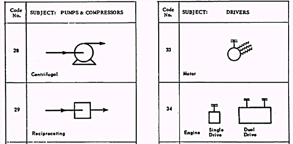
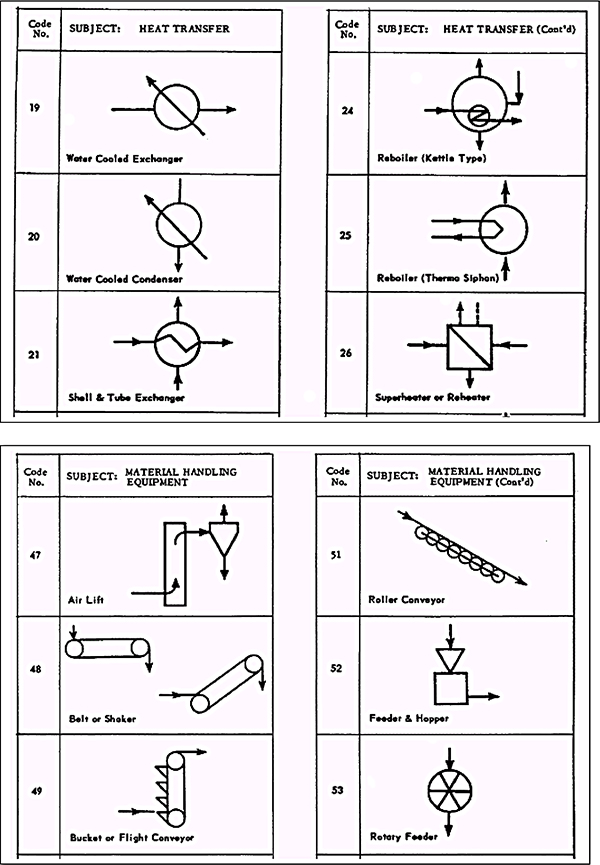
Instrumentation drawings and diagrams
Instrument numbering (tagging)
Instrument Tag Nos.
As with Equipment numbers all instruments (including virtual instruments that exist in a DCS, PLC or other shared system) are given unique identifiers called tag numbers. The ISA tagging system is virtually universally adopted in terms of the basic construction of a tag number. The ISA system comprises a group of alpha characters which describe both the variable being measured (or controlled) together with the broad characteristics of the instrument itself. The first alpha character in the tag always identifies the physical variable with which the instrument is associated (e.g. Pressure, Temperature, Flow etc). Subsequent alpha characters identify the function of the instrument and may be comprise more than one additionally character. Hence FIC would refer to a Flow Indicating Controller, PAHL would refer to an alarm device on pressure with both High and Low alarm settings. Once the basic alpha tag characters are established a group of numeric characters are added to identify the loop number. These may be 3 or 4 or more numerals but all devices interconnected on the same loop must have the same loop number – the individual instruments are therefore differentiated by their alpha character functionality. As with the equipment numbering system large plants employing an Area numbering scheme may add the plant area number in front of the tag to create the full tag number. As an example tag number 100PT001 and 100PIC001 are respectively a pressure transmitter and a pressure indicating controller in plant area 100 on loop number 001. The table below lists the ISA alpha character system.
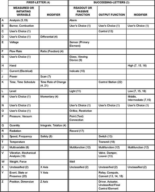
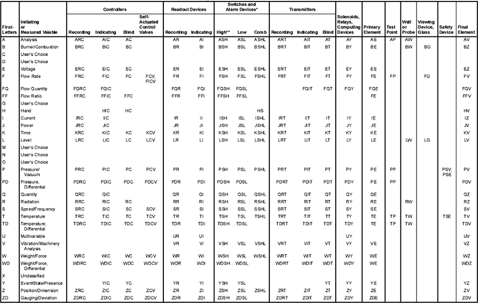
Instrument symbols
Bubbles
The ISA standard employs a simple system to identify instruments on process drawings by using “bubbles” – the terminology originating from the fact that the original symbol set used circles exclusively. The symbol set has now been expanded to account for the emergence of shared systems such as DCSs, PLCs and host software systems which all have multiple levels of functionality within one box. The system endeavors to identify the location of the instrument function (field, control room, auxiliary panel etc) and when used in conjunction with the instrument tag gives the reader of a diagram a clearer understanding of the overall control loop and strategy. The ISA bubble symbol set is shown in the attached table.
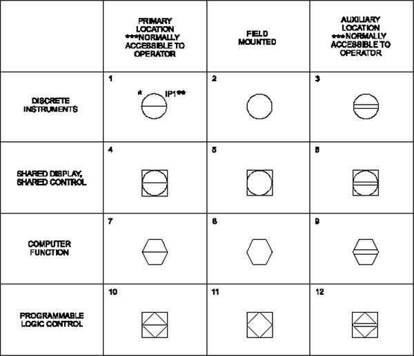
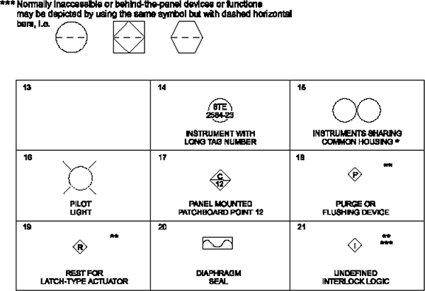
Primary and final elements
The ISA standard recognizes that many primary and final elements cannot be fully described by a bubble and tag number alone and therefore caters to the use of a wide variety of symbols to show the technology associated with a primary or final element. An example of these symbols is shown in the tables below.
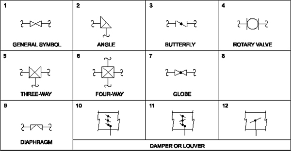
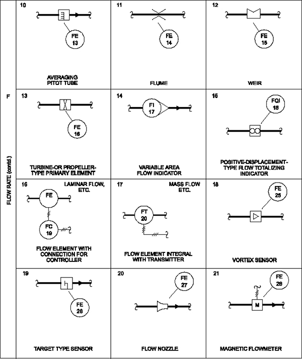
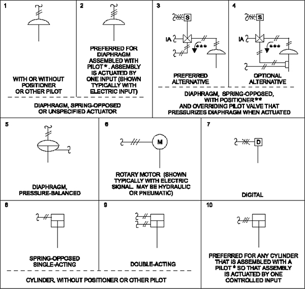
Extended functionality
The ISA standard further recognizes that certain instruments may have a complex or unique functionality that cannot be full described by a tag number and bubble and to this end it allows for the inclusion of a small box/boxes outside the bubble with a symbol to identify the specific detail of the instrument. A representative table of ISA functionality legends appears below.
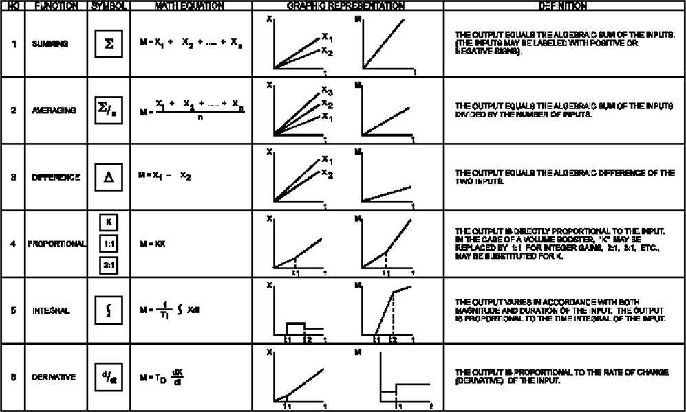
The SAMA system
The Scientific Apparatus and Manufacturers Association further expands on the ISA extended functionality system by using a range of blocks linked together to describe the functionality within a control loop. Although seldom employed these days it provides a useful tool for identifying control and measurement functions within complex loops. A table of SAMA functions and an example of the scheme are shown below.
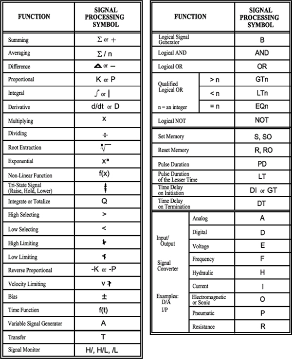
Example of a SAMA Scheme for describing the control strategy of a 3-element boiler drum level control system.
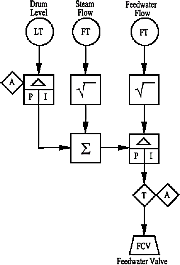
Instrument interconnections
The ISA standard also provides for the interconnection of bubbles to show, on process drawings, the media by which they communicate – be it pneumatic, electrical, non-contact etc. The table below lists how the bubbles are interconnected.
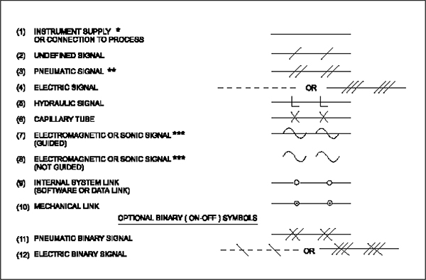
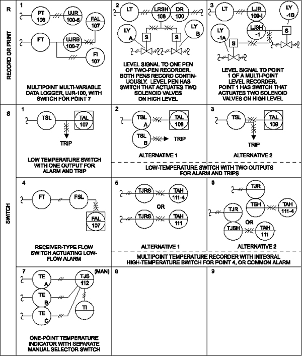
Electrical drawings and diagrams
Electrical equipment numbering
Component numbering
Components of an electrical circuit are numbered by means of a single alpha character combined with a sequential digit each time a component of a new type is used. The standards for the alpha character may vary from company to company and it is normal to draw a legend sheet to explain the use on a particular set of drawings. The attached table broadly coincides with the recommendations of the IEC Publication 27 standard for letter designations.
| Letter Code | Type | Examples |
| A | Assemblies, subassemblies | Amplifier with transistors, magnetic amp, laser |
| B | Transducers, from mechanical to electrical and vice versa. | Thermo electric sensor, transducer, loudspeaker |
| C | Capacitors | |
| D | Delay / storage devices | Bi-stable, mono-stable, register |
| E | Miscellaneous | Lighting and heating devices |
| F | Protective devices | Fuse, arrestor |
| G | Generators, supplies | Battery, supply device |
| H | Signaling devices | Optical and acoustic indicators |
| J | ||
| K | Relays, Contactors | |
| L | Inductors | Induction coil, line trap |
| M | Motors | |
| N | Amplifier, regulator | |
| P | Measuring/Test equipment | Indicating, recording devices |
| Q | Mechanical switching devices | Circuit breaker/isolator |
| R | Resistors | Potentiometer, rheostat, shunt, |
| S | Switches, selectors | Pushbutton, limit, selector |
| T | Transformers | Voltage, current transformer |
| U | Modulators, changers | |
| V | Tubes, semiconductors | Diode, transistor, |
| W | Transmission paths, waveguides, aerials | Jumper wire, cable, busbar, dipole |
| X | Terminals, plugs, sockets | Socket, test-jack |
| Y | Electrically operated mechanical devices | Brake, clutch |
| Z | Terminations, hybrid transformers, filters, equalizers |
Single line symbols
IEC Publication 617 provides an extensive range of symbols which are used in electrical circuits. These are normally employed in both single line and electrical schematics but differ from those symbols employed in ladder logic schematics. Typical examples of the IEC symbol set are shown below.
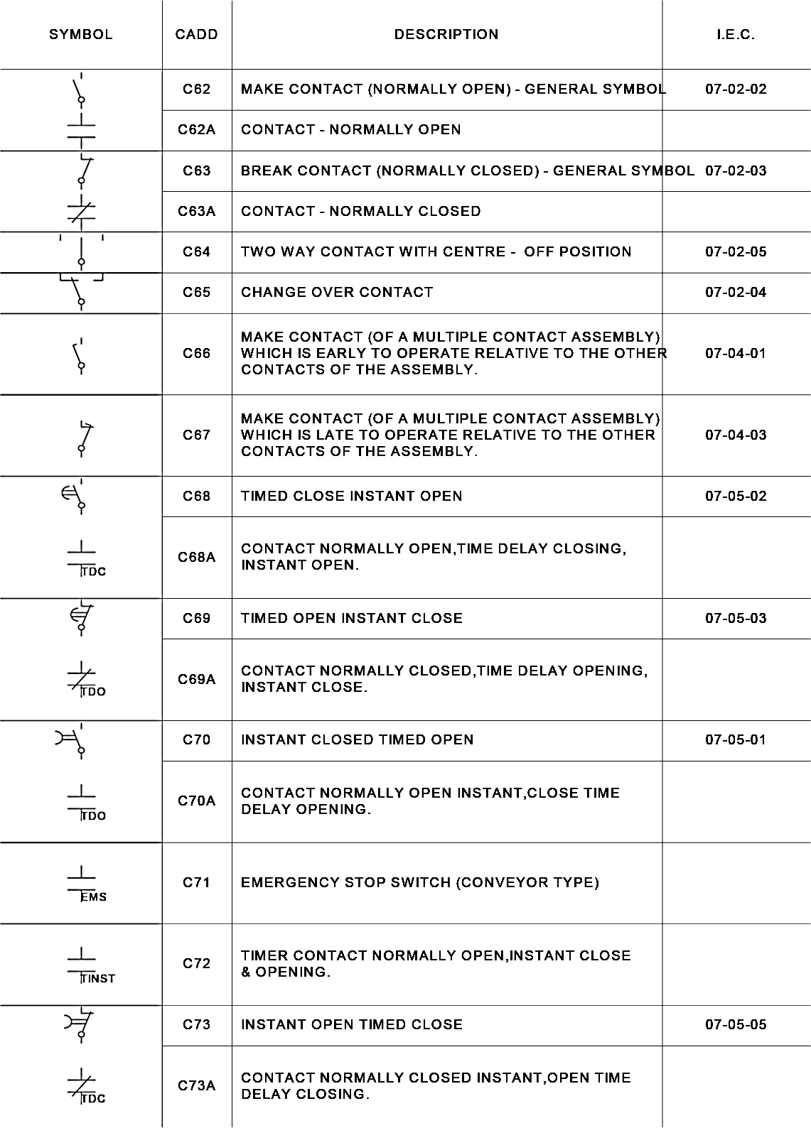
2.5.3 Wire numbering system
Although there is no set standard for wire numbering of electrical circuits the generally accepted rules are to use a numeric system with 3 (or more) digits in which the number increments each time there is a break in the circuit (i.e. terminal, fuse etc).
The reader should be aware that there are individual country standards (e.g. AS3000 – Australian Wiring Rules) that govern the use of certain letters (e.g. L, A, N, E) in wire numbering systems involving potentially lethal voltages.
Practical Exercises
Note that a selection of these practical exercises will be undertaken, not all of them. The selection depends on the particular group in the class and does not include all of these due to time constraints.
Practical 1
Pressure Testing
1.1 Objectives
- To check, range and calibrate various types of indicators and 4-20mA pressure transducers.
1.2 Equipment required for all exercises
- Pressure generator (on mounting board) comprising
SMC digital pressure switch ISE30A-01-N-F (incorporates
own pressure transducer) PT 104 - Bourdon tube mechanical type indicator
55mm dia, oil filled Austral KL.1,6
OR PI 101 - Bourdon tube mechanical type indicator
90mm dia, oil filled Stewart-Buchanan make PI 105 - Endress and Hauser PMP 46 Pressure Transducer PT 102
- Rosemount model 3051 DP pressure transmitter PT 103
- Connecting cables and pressure tubing
- Multimeter (various makes and models; must be digital)
- Conlog 4001 calibrator
- File containing copies of makers’ manuals
1.3 Procedure – Bourdon Tube pressure indicator PI 101 or PI105
Check equipment details:
Tag no.: PI 101 or PI105
Supply 24 VDC power to the board via terminals (D) and (E).by connecting the battery eliminator to 240 VAC mains. Check that the SMC pressure transducer display is lit up.
If not already done, set the pressure transducer to read kPa as follows:
Press the “s” button for 2 sewconds or longer until the function [F0] is displayed. Then press “s” and use the UP DOWN button to select the desired display units. For kPa the display will show “PA”. Then set this by pushing “s”.
With [F0] displayed again hold the “s” button for more than two seconds to return to measurement mode. Refer to page 23 of the ISE30A-01-N-F manual if necessary.
Note the readings on both the indicator (PI 101 or PI 105) and the LED display. The LED display acts as the calibrator for this exercise.
Note the reading with the indicator tubing unplugged. Record these two values in the table.
Now connect the pressure indicator to port (A), the open port of the second pressure release valve on PT104 with the 6mm tube supplied. (To disconnect the tube from the fitting at any time, first push the fitting’s plastic insert inwards and then pull gently on the tube).
Now pull on the metal handle connected to the cylinder shaft whilst watching the LED display. Set an LED value of close to 200kPa. Again note the readings on both the indicator (PI 101 or PI 105) and the LED display.
Repeat the exercise for a third time with an approximate value of 400kPa.
In the table determine the difference between the indicator and the calibrator and calculate the inaccuracy as a percent of the indicator span.
| Calibrator pressure (kPa) LED | PI 101 or PI 105 pressure (kPa) | Error (%) |
| 0 | ||
1.4 Procedure – Measuring cell pressure transmitter PT 102
Check equipment details:
| Tag no.: | PT 102 |
| Manufacturer: | Endress + Hauser |
| Model: | PMP 46 – RE 17M2HCDLE |
| Serial: | 4113D001024 |
| Range: | 0-1600 |
| Tag no: | PT104 |
| Manufacturer: | Pressure generator (on mounting board) comprising SMC digital pressure switch |
| Model: | SMC ISE30A-01-N-F |
Make the two electrical power connections between the PT 102 and PT104by connecting the pressure transmitter terminal 1(+) red to terminal (D) and 2(-) blue to terminal (E) on the pressure generator.
Set the scale of a multimeter to read 20mA. Connect the red output wire to the +ve terminal of the multimeter and the white output wire to the –ve terminal.
(see Figure E1.1 below).
Read the initial pressure (0 kPa) and check that the transmitter output is 4.0mA using a multimeter.
Make an air pressure connection between PT 102 and PT 104 (port A) using the 6mm blue plastic tubing and quick-release fittings.
Make sure both shut-off valves on PT 104 are open. Pull gently on the handle of the air cylinder. By doing this carefully set the pressures in the table below on the SMC LED transmitter display.
Note the required output currents and record them in milliamps for each 10% of pressure span. Plot these values using graph paper to confirm linearity of the transducer and transmitter.
Calculate the error as a percentage of the span. (Span in this case 20-4=16mA)
| Set Pressure (kPa) | Required current (mA) | Measured current (mA) using multimeter | Error (%) |
| 0 | 4 | ||
| 25 | 5.6 | ||
| 50 | 7.2 | ||
| 75 | 8.8 | ||
| 100 | 10.4 | ||
| 125 | 12.0 | ||
| 150 | 13.6 | ||
| 175 | 15.2 | ||
| 200 | 16.8 | ||
| 225 | 18.4 | ||
| 250 | 20.0 |
Refer to the Manufacturers brochure for the following:
What sensing principle does PT102 use?
What types of pressure can this device measure?
– Gauge
– Absolute
– Differential

1.5 Procedure – Rosemount Pressure transmitter PT 103
Check equipment details:
| Tag no.: | PT 103 |
| Manufacturer: | Rosemount |
| Model: | 3051C |
| Range: | 0-50kPa |
| Tag no: | PT104 |
| Manufacturer: | Pressure generator (on mounting board) comprising SMC digital pressure switch ISE30A-01-N-F (incorporates own pressure transducer) |

IMPORTANT: Locate and identify the H and L fittings on the base of the transmitter. The H indicates the high-pressure side (blue connector) and the L indicates the low pressure tapping side (orange connector).
PART 1.
Make the electrical connections between the transmitter and the calibrator; connecting the pressure transmitter +ve terminal to (D) and -ve to (E) on the “Xmtr” terminals on the pressure generator PT104. Put the multimeter, set on the 20mA scale, in series with these connections, observing the correct polarity. (see attached diagram).
Open the release valve on PT103 (the one in the central nut in the lower part of the transmitter, to the rear of the instrument, marked “U”). Check that its display reads 0 kPa. If not, adjust the transmitter zero by swinging aside the metal cover on the top of the unit by releasing one screw. Turn the “Z” switch (plug) only until free and hold for 2 and 10 seconds. If this does not zero, note the displayed KPa value. DO NOT touch the SPAN switch on this unit.
Connect the pressure calibrator port to the HIGH side of the Rosemount pressure transmitter using �” pipe. Close the PT103 transmitter release valve and ensure both shut-off valves on PT104 are open. (They are in series)
Using hand pump, set the pressure until the multimeter reading 20mA. Check the pressure reading on the LED display panel of the SMC switch. The display on the transmitter should also indicate this reading.
Note: This should read 100kPa. Do not exceed this reading, otherwise the display will generate a “press range” error signal.
As before, check and record the milliamp values of output for each 10% of pressure span on the table below. Plot these values to confirm linearity of the transducer and transmitter.
| Range | Required current (mA) | Measured current (mA) |
| 0% | 4 | |
| 10% | 5.6 | |
| 20% | 7.2 | |
| 30% | 8.8 | |
| 40% | 10.4 | |
| 50% | 12.0 | |
| 60% | 13.6 | |
| 70% | 15.2 | |
| 80% | 16.8 | |
| 90% | 18.4 | |
| 100% | 20.0 |
PART 2.
Zero the pressure in the system with the pressure release valve.
Connect the pressure calibrator to the LOW (blue) side of the Rosemount pressure transmitter using blue ¼” tube.
Set a pressure of about 25 kPa.
What are the differences between the calibrator pressure readings and the transmitter pressure readings?
Refer to the manufacturer’s brochure for the following:
What is the sensing principle used?
What types of pressure can this device measure?
– Gauge
– Absolute
– Differential
Practical 2
Level measurement with Ultrasonics
2.1 Objectives
- To demonstrate the use of ultrasonics in level measurement.
- To determine a suitable range of operation and provide a 4-20mA signal for that range.
2.2 Equipment Required
- Endress & Hauser FMU 40-ARB2A2 transmitter probe mounted
on tripod LE 201 - Adapter Box LT 201
- Tape Measure LI 202
- Multimeter 24V DC power supply
2.3 Ultrasonics configuration and familiarization
Often the requirement for level sensing may require that a non-contact and non-intrusive means may be required.
This may be due to a number of factors such as:
- temperature
- nature of the material
- distance
One of the most common types of non-contact sensors is the ultrasonic level measurement.
Procedure
Make connections as shown in Figure 1:

Unscrew the grey retaining ring of the display and put to one side. Apply power to the ultrasonic level transmitter and check that the display is operating.
On power up the FMU 40 executes a self-test and then displays the configured display parameter (e.g. distance, measured value, etc).
Using the local display pushbuttons on the FMU 40 allows the configuring and viewing of all measured values and configuration parameters.
To enter the configuration mode press the enter button (‘E’) once.

From the ‘Group Selection’ menu scroll up/down using the +/- keys until the ‘basic setup’ menu is highlighted – select by pressing enter once.
The menu will now take the user through a series of steps with each step requiring an option be selected – pressing enter at each selection takes the user to the next step.
Set up the FMU40 to the following conditions:
‘tank shape – no ceiling’
‘medium property – liquid’
‘process condition – calm surface’
‘empty calibration – 5.000 metres’ (the decimal vale is entered separately)
‘blocking distance – 0.25 metres’ (note this is a default value for this unit)
‘full calibration – 4.75 metres’
The unit will now display both the distance and measured values. Now determine whether the reading is correct or not. Press enter to continue.
‘Check distance – distance OK’
The unit will now map various echoes to allow fine tuning and elimination of any false echoes which may be present.
‘Range of mapping – 0.415m’ (leave the defaulted value as is for the moment)
‘Start mapping – on’
The unit will now proceed to map echoes – once completed, press ‘Enter’.
The unit will now display both distance and measured values.
Press BOTH ‘+’ & ’-’ buttons simultaneously to exit configuration and enter run time.
Angle the transducer black sensor cylindrical cover vertically down towards the floor, (or towards a wall) with no objects between the transducer and the wall. This is intended to measure level by raising and lowering the tripod stem.
Note that when the tripod stem is fully retracted, then a high level is simulated. When the stem is fully extended, this is the low level. There is no need to adjust the tripod legs for this exercise.
The response time needs to be configured (although default settings work well in most applications). Note that setting a response quicker than that of the system can lead to spurious errors in measurement. A too slow response can make the system difficult to control in closed loop applications. Refer Step 3, P003. 10m/min will work well for our application since it is not critical control.
The transmitter’s transducer is a XPS-15 and should be set up with parameter no. 4 containing the value 104. Refer Step 4, P004.
Measurement units may vary. The SI Standard is metres. To obtain a higer resolution millimetres (mm) can be used.
Alarms trips and other operational limits also operate as a percentage of the range of operation.
Configure the operating range of the system as follows:
For this exercise, when the tripod stem is extended to its highest, this will be considered the low level or the tank’s empty state.
Set the system to the empty state by ensuring that the tripod stem extension is wound down. (Please release the locks on the tripod first and do not use excessive force!) Note the distance using the tape measure. Enter this distance into parameter P006.
Retract the tripod stem to the minimum height. (Releasing the lock first!) This is considered the high level, or Tank Full state.
Note the difference between the high and low level readings ( about 350mm? ). This is the span or operating range of the system. Enter this distance into Parameter P007.
| P001 | 1 | Level – How full the vessel is |
| P002 | 2 | Solid Process material |
| P003 | 3 | Fast response –10m/min |
| P004 | 104 | (Head Type: XPS-15) |
| P005 | 3 | units of measurement – mm |
| P006 | Low Level | Value |
| P007 | Span | Value |
2.4 Calibration of the 4-20mA output
Most ultrasonic units will monitor and indicate the level in the engineering units without much configuration required. However in a control system, or to other display devices the information can be sent by means of a 4-20mA signal. For this milliamp signal to be of use, the range needs to be configured to represent the level.
This unit can measure from 0.3m to 9.6m. If however the range of operation is quite small then the resolution and accuracy of the signal can be increased by reducing the range of the signal (4-20mA) to that of the system.
Refer to the users manual for the level transmitter and configure the 4-20mA output for the range of operation as defined above.
| P200 | 2 | Select 4-20mA output |
| P201 | 1 | Level measurement |
| P202 | 1 |
Remember:
– The low level occurs when the stem is fully extended and should show 0% – 4mA.
– The high level occurs when the stem is fully retracted and should show 100% – 20mA.
Check the operation as follows:
Pressing the [5/mA] key when in RUN mode will display the output current in the Auxiliary reading window.
Vary the height of the transmitter and check the following:
Correct mA signal at low level
Correct mA signal at mid range
Correct mA signal at high level
2.5 Additional Exercises
Using the FMU40 instruction manuals the user is now encouraged to explore further functionality of the FMU40 including the following:
- What happens when an object is placed within the blocking distance of the unit?
- How do you change the displayed value from ullage to level?
- What happens when you setup a safety distance of 0.4 metres?
- What does the linearization function do?
- Plot the envelope curve and explain what is causing any other reflections? Is it possible for secondary reflections to have a greater amplitude than the primary reflection?
Note: Use of pictures and texts extracted from the Prosonic M instruction manuals have been done so with the kind permission of Endress & Hauser.
Practical 3A
Temperature (using the DataTaker DT80)
3.1 Objectives
- To calculate the response time for different thermocouple and RTD installations.
You may already find that the hardware connections have been made by a previous group. However please check that they are correct.
3.2 Equipment required:
- 1 x K Thermocouple (sheathed or enclosed) TT 301
- 1 x K Thermocouple (bare) TT302
- 2 x RTD – Pt 100 ( TT 303, TT 304
- 2 x Thermowells for the 2 x RTD’s (one with thermopaste and one without)
- Ice bath (or cold water)
- Boiling Water in container (or hot water)
- Datalogger (DT80)
- Computer (eg ACER Notebook)
- DeLogger Datataker software resident on computer
- 2 x Thermowells
- Thermopaste
- USB Communications Connecting cable (Computer to Data Logger)
- Small screwdriver suitable for screw terminals of Data Logger
3.3 Temperature response and accuracy
The response time is the time it takes to get to 63.2% of the final settling value. This is independent of the range of the device. If the device were a Pt 100 with a range of operation of -200 to 630oC and the temperature being monitored changed from 100 to 200 oC, then the response time would be the time it takes to go from 100 oC to 163.2 oC.
3.3.1 Procedure
Hardware Setup
- Collect all hardware and software components defined above.
- Connect the Serial communications cable supplied to the data logger RS232 port and to the Computer Serial port.
- Connect the power cable to the personal computer and power it up.
- Connect the Plug pack power supply to the data logger using the supplied plug and power cable. Be careful to observe polarity of the power connections.
- Plug the power supply into the mains supply and power on the data logger. The display on the logger should flash on and off.
- Click on DeLogger icon on desktop.
- You will then see a bewildering number of screens to select from. Select the Text1.dlt by clicking on it from the list of programs (Form1.dlf, Chart1.dlc, Text1, dlt,…Prog1.d80). Maximise the Text1.dlt to view better.
- At the Toolbar at the top of the screen (File Edit View Connections��.Help) Select Connections and then Connect. Select Serial Port1 under Connection. Click OK. You will receive confirmation that you have selected the correct settings when you hear the DataLogger relay clicks.
Please read Note1 at the end of this write-up if you cannot initiate communications between logger and computer.
- Your DeLogger Text1.dlf will be broken up into three windows:
- The Top windows which gives the datalogger responses (displays data returned from the data logger)
- The middle windows which is where you will type in commands (see later but to be sent to the data logger).
- The bottom windows which reports errors and status in the communications with the logger.
Resize the top and middle window of Text1.dlf so that each are approximately a third of the computer screen; to make for easier reading.
Go to the middle window and type in:
RESET <Enter>
A pop up screen will then ask you if you want to “Connect to the selected site”. Click Yes and select Serial Port 1 on the connection selection drop down menu below this pop up screen.
Sending commands to the Data Logger
- The currently highlighted line of information in the middle window can be sent to the data logger by entering the commands and hitting the <Enter> key
Obtaining Readings
- The best way to achieve this is by creating a whole series of readings which will be taken at regular intervals. To perform this task a schedule is sent to the logger. A schedule is a list which tells the device which channels to read and when.
- A standard reporting schedule which reads the thermocouple temperature and voltage on channel 1 every second, can be sent to the data logger by sending the command line:
RA1S 1TK 1V <Enter>
The meaning of the ASCII character sequence which makes up the schedule command is as follows:
- RA1S is the schedule command to report schedule A (or scan the channel list) every 1s.
- 1TK is the channel command to read the K-type thermocouple temperature on channel 1.
- 1V is the channel command to read the differential voltage input on channel 1.
- Additional channels may be added and read simultaneously e.g. RA1S 1TK 4TJ
- To temporarily halt the schedule RA send the command line:
HA <Enter>
- To continue send the command line:
GA <Enter>
Thermocouples
Connect the K-type sheathed thermocouple TT 301 to channel 2 of the data logger as shown in the figure below.
Check equipment details:
| Tag no.: | TT 301 |
| Model: | K-type thermocouple |
| Details: | Sheath – Yellow |
| Positive – Yellow | |
| Negative – Red |
The ANSI MC96.1 standard for thermocouples and extension wire specifies that for ‘K’ type thermocouples the outer cover is yellow and the terminals are as follows:
– Positive (+) terminal is yellow.
– Negative (-) terminal is red.
Ensure that each lead is correctly positioned and securely tightened by the (+) and (-) screw terminals of channel 2.
How can you distinguish quickly between a thermocouple and RTD using a multimeter?
(Clue: Resistance of a RTD will be about 100 Ohms and thermocouple will be a few ohms).
The differential measurement configuration shown is most commonly used where the signals from the sensor/transducer are very small and more susceptible to the effects of noise and/or where the cables from the transducer to the measuring equipment are very long and also more susceptible to noise.

Differential Thermocouple Configuration
In order to make a simultaneous continuous temperature measurement type the following at the highlighted command bar:
RA2S 2TK <Enter>
Try and interpret the flood of readings that come back from the data logger. These responses can be simplified; but the key parameters will be the last values on each line of the response from the logger.
Now connect the unsheathed K-type thermocouple to channel 3 and repeat the exercise. Adjust the commands for the new channel number. What do you notice ?
Now compare the response times for the two thermocouples in moving from ice to the hot water for the measurement to “settle down”. What do you notice ?
Remove the thermocouples after you have completed this practical session.
Examine the influence of thermowells on RTD response
Connect the RTD (with thermowell with no thermopaste) to channel 1 of the data logger using the four-wire configuration as shown in the figure below.
Check equipment details:
| Tag no.: | TT 303 |
| Model: | RTD |
| Type: | Pt100 |

Four-wire RTD input.
In the four wire configuration two excitation leads carry the constant excitation current which flows through the RTD. The value of this current should remain constant irrespective of the excitation lead resistance or the resistance of the RTD.
The other two measurement leads are used to measure the voltage drop across the RTD. The actual current flowing in these leads is very small due to the very high input impedance of the voltage measurement circuit. Therefore, voltage drops across the lead resistances are so small they can be assumed to be negligible.
Now connect up channel 2 of the data logger with the second RTD (which is in a thermowell with thermopaste). Add more thermopaste if necessary. DO NOT get the thermopaste on your clothes. Keep a box of tissues nearby to clean the “stuff” off.
Check equipment details:
| Tag no.: | TT 304 |
| Model: | RTD |
| Type: | Pt100 |
Create a schedule of readings by typing:
RA2S 1PT385(4W) 2PT385(4W)
Take the RTD in a thermowell (but with no thermopaste) connected to channel 1 and see how long it takes to stabilise in being moved from the ice bath to the hot water. Repeat the exercise with the RTD in the thermowell connected to channel 2 but with thermopaste. (Be careful with the thermopaste. It is very gluey!)
Note 1:
If you cannot establish communications with the Comm port listed you need to create a USB connection. First of all run the USB patch program to run the drivers.
Go to Connection in top row in DeLogger.
Click Properties
Click on New
Type in USB Port1 under Connection Name
Under settings for PC USB Port click on the “…” symbol and select USB (USB) – FTDI.
Initiate a forced connection (If necessary) back under the connections selection box.
Practical Exercise 3B
Temperature (using Datataker DT50)
3.1 Objectives
- To calculate the response time for different thermocouple and RTD installations
- To compare extension leads with compensation leads
There are two sections to this practical exercise.
You may already find that the hardware connections have been made by a previous group. However, please check that they are correct.
3.2 Equipment required
- 1 x K Thermocouple TT 301
- 1 x J Thermocouple TT 302
- 2 x RTD – Pt 100 TT 303, TT 304
- Ice bath
- Boiling water in container
- Datalogger and laptop computer OR Conlog 4001 Calibrator
- 2 x Thermowells
- Thermopaste
- Small screwdriver suitable for screw terminals of Data Logger
- Thermocouple connected to both extension (TT 305) and compensation leads (TT 306)
3.3 Temperature response and accuracy
The response time is the time it takes to get to 63.2% of the final settling value. This is independent of the range of the device. If the device were a Pt 100 with a range of operation of -200 to 630oC and the temperature being monitored changed from 100 to 200 oC, then the response time would be the time it takes to go from 100 oC to 163.2 oC.
3.3.1 Procedure
Hardware Setup
- Connect the 9-pin D-type male connector of the communications cable supplied, to the data logger 9-pin female RS232 Communications socket.
- Connect the other 9-pin female connector to either the COM1 or COM2 port of the Personal Computer.
- Power up the Personal Computer.
- Connect the Plug Pack power supply to the data logger AC/DC terminals. Although the output of the power supply is AC it doesn’t matter which lead goes into which terminal as the terminals are polarity independent. (Be careful not to short circuit the Plug Pack terminals!)
- Plug the power supply into the mains supply and power on the Data Logger. The LED on the logger should flash on and off.
- Start the DeTerminal Program by changing to the DT subdirectory and typing DT <ENTER> at the DOS command prompt. The sequence of characters should be as follows:
CD\DT <ENTER>
DT <ENTER>If the Data Logger has been found connected correctly you will first get the user message:
Found at 4800 baud
The DeTerminal Program will then show a user screen which has two windows. The top window displays data returned from the Data Logger, and from now on will be referred to as the data window. The bottom window is used for typing commands to be sent to the Data Logger and will be referred to as the command window. Both these windows can be scrolled, saved and cleared.
Sending commands to the Data Logger
- The currently highlighted line of information in the command window can be sent to the Data Logger by pressing the <ALT> and <L> keys together. This combination of keys is known as the Send Line command.
- If you want to toggle between the screen windows, you can use the <TAB> key controls movement between the two screen windows. The active window can be identified by the options showing at the top border of the window.
Obtaining Readings
- The best way to achieve this is by creating a whole series of readings which will be taken at regular intervals. To perform this task a schedule is sent to the logger. A schedule is a list which tells the device which channels to read and when to read them.
- A standard reporting schedule which reads the thermocouple temperature and voltage on channel 5 every second, can be sent to the Data Logger by sending the command line:
RA1S 5TK 10V <ALT> <L>
The meaning of the ASCII character sequence which makes up the schedule command is as follows:
- RA1S is the schedule command to report schedule A (or scan the channel list every 1s)
- 5TK is the channel command to read the K-type thermocouple temperature on channel 5
- 10 V is the channel command to read the differential voltage input on channel 10
- Additional channels may be added and read simultaneously e.g. RA1S 5TK 4TJ
- To temporarily halt the schedule RA, send the command line:
HA <ALT> <L>
- To continue, send the command line:
GA <ALT> <L>
Thermocouples
Connect the K-type sheathed thermocouple TT 301 to channel 5 of the Data Logger as shown in the figure below.
Check equipment details:
| Tag no.: | TT 301 |
| Model: | K-type thermocouple |
| Details: | Sheath – Yellow |
| Positive – Yellow | |
| Negative – Red |
The ANSI MC96.1 standard for thermocouples and extension wire specifies that for ‘K’ type thermocouples, the outer cover is yellow and the terminals are as follows:
– Positive (+) terminal is yellow.
– Negative (-) terminal is red.
Ensure that each lead is correctly positioned and securely tightened by the (+) and (-) screw terminals of channel 5.
The differential measurement configuration shown is most commonly used where the signals from the sensor/transducer are very small and more susceptible to the effects of noise – and/or where the cables from the transducer to the measuring equipment are very long and are also more susceptible to noise.

Differential Thermocouple Configuration.
In order to make a simultaneous continuous temperature measurement, type the following at the highlighted command bar:
RA2S 5TK 4TJ <ALT><L>
Next, connect in the J-type sheathed tip thermocouple to channel 4 using the same procedure as above. (The cover is black, the positive terminal is white, and the negative terminal is red).
Check equipment details:
| Tag no.: | TT 302 |
| Model: | J-type thermocouple |
| Details: | Sheath – Black |
| Positive – White | |
| Negative – Red |
Next, compare the response times for the two thermocouples in moving from ice to the hot water for the measurement to “settle down”.
Examine the influence of thermowells on RTD response
Connect the RTD (without thermowell) to channel 1 of the Data Logger using the four-wire configuration as shown in the figure below.
Check equipment details:
| Tag no.: | TT 303 |
| Model: | RTD |
| Type: | Pt100 |

Four-wire RTD input.
In the four wire configuration, two excitation leads carry the constant excitation current which flows through the RTD. The value of this current should remain constant irrespective of the excitation lead resistance or the resistance of the RTD.
The other two measurement leads are used to measure the voltage drop across the RTD. The actual current flowing in these leads is very small due to the very high input impedance of the voltage measurement circuit. Therefore, voltage drops across the lead resistances are so small, that they are assumed to be negligible.
Now connect up channel 2 of the Data Logger with the second RTD.
Check equipment details:
| Tag no.: | TT 304 |
| Model: | RTD |
| Type: | Pt100 |
Create a schedule of readings by typing:
RA2S 1PT385(4W) 2PT385(4W)
Take the RTD in a thermowell (but with no thermopaste) connected to channel 1 and see how long it takes to stabilise after being moved from the ice bath to the hot water. Repeat the exercise with the RTD in the thermowell connected to channel 2, but this time, use thermopaste. (Be careful with the thermopaste. It is very gluey!)
3.4 Thermocouple extension leads compared with compensation leads
There are two basic means of increasing the distance for which a thermocouple can be located from a transmitter.
The two types of leads are:
- Extension leads
- Compensation leads
Extension leads are typically of the same material as the thermocouple junction, whereas compensation leads are made from copper or a copper alloy.
Procedure
Connect up a thermocouple which has both extension leads and compensation leads connected to it.
Check equipment details:
| Tag no.: | TT 305 |
| Model: | K-type thermocouple with extension leads |
| Details: | Sheath – Yellow |
| Positive – Yellow | |
| Negative – Red |
| Tag no.: | TT 306 |
| Model: | K-type thermocouple with compensating leads |
| Details: | Sheath – Red |
| Positive – Brown | |
| Negative – Red |
Identify which is a compensation lead and which is an extension lead. Confirm the type of thermocouple.
Using the procedure as before, connect the extension leads to the channel 3 on the Data Logger and the compensation leads to channel 4 on the Data Logger.
Use the commands:
RA1S 3TK 4TK <ALT> <L>
Measure ice bath and hot water temperature with both set of leads and compare results.
What do you notice?
Practical 4
Flow Control Loop
(PC-Control Lab Software)
Getting started with PC-ControlLAB
1 Introduction
To get started on the simulation exercises you will first need to install PC-ControLAB on your PC and ensure that you are familiar with the tools and controls it provides. The software will be provided by your instructor on an installation CD supplied by IDC Technologies for your temporary use for the duration of the workshop and for a limited follow up period thereafter by means of a short term license key.
All the procedures required to get started are set out in the PC-ControLAB Quick Start Guide which is provided overleaf. This guide is also available as a PDF file in the CD package. The package includes a tool called “Builder” which is used to configure and modify simulations. This is very useful for you to inspect the models provides and to modify them if you wish.
The software is supplied with a suite of data files for training exercises.
2 Installing IDC exercise data files.
The IDC files are all contained in the folder to be supplied by IDC called “IDC PC Models” To install these files for use in the exercises proceed as follows:
- Start PC-ControLAB and select the command “PROCESS” then “SELECT MODEL”.
- The window opens to show a list of files.
- Copy the folder “IDC PC Models” and paste it into the files folder. The models will then be available by selecting the subfolder.
- In some exercises the instructions will call for a control strategy file (.stg) these files will be included with the above folder.
3 Tutorial
We recommend that as soon as you have installed PC-ControLAB you should work through the following 4 sheets of the “Quick-start Guide” and then you should go the “HELP” command and work through the sequence of tutorial exercises provided there before proceeding with the practical exercises. The Tutorial and Help files provide very useful descriptions of all the most commonly used configuration blocks for control systems.
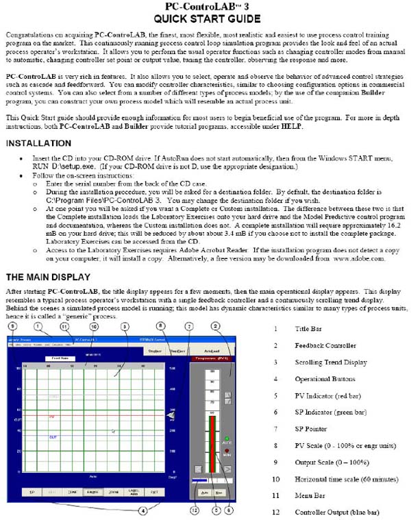


Before you start
To get started with the exercises you will first need to install PC ControLAB and the load the exercise data files all as described above.
The following is a reference list of the data files required for the exercises.
| Exercise No | PC Pracs Folder | File Name |
|---|---|---|
| 1 | EX-1 | IDC Flow 1.mdl |
| 2 | EX-2 | IDC Flow 1.mdl |
The data files provide the process model for each exercise and in some cases strategy files are used to preload controller settings. Details of how to start up each exercise are contained in the instruction steps given in the practical exercise sheets starting overleaf.
Exercise 4a
Flow Control Loop – Basic Example for Open Loop Control
1.1 Objective
This exercise will familiarize the student with the basic concepts of open loop and closed loop control. It provides an opportunity to get a first feel for the open loop response of the process being controlled. A flow control loop as shown in figure 1.1 below will serve as a practical example for this exercise. A flow control loop is generally not difficult to operate and illustrates the basic principles effectively.
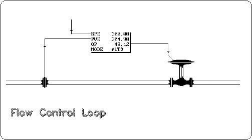
Basic Flow Control Loop
1.2 Operation
Since this is a relatively simple exercise, it can be used for familiarization with the principles of operation of the simulation software: “PC Control-Lab”. Firstly, you must ensure that you have installed the PC Lab software by following the instructions provided in the introduction. You should also have completed some of the first parts of the tutorial (Under HELP) to ensure you are familiar with the basic controls and operations. Then proceed with the following steps.
Step 1: Start the program in MS Windows by running PC-ControLab
Step 2: Open the project file for IDC Flow 1.mdl which is a pre-configured flow control loop with first order lag and dead time.
- Click on Process | Select Model.
- Select the file location “PC-Pracs” and then subfolder “Ex-1” Highlight “IDC Flow 1.mdl “and press Open.
- Set the Horizontal grid scale to “Seconds” (under View). NB: Most exercises in this workshop use the SECONDS scale. This has to be selected at the start of each exercise
- Set the LOAD value to 65% on screen by pressing STEP INCR
- Set the controller mode to Manual
- Use the OUT key to set the OUT value = 30%
You should now have a display on screen that simply indicates the output value to the control valve is steady at 30% and the PV is steady at 105 m3/hr as per Figure D1.2 below

Initial display for flow loop manual mode testing showing trend display (left) and controller faceplate display (right).
This display gives a general idea of the process and displays the major variables PV (process variable scaled 0 to 300 m3/hr) and OP (controller output signal to flow control valve scaled in range 0 to 100%). The SP (set point) is shown as an arrow on the right of the trend screen and as a red bar on the controller faceplate.
Note that the operating data with PV, SP and OP appears in a box on the left side whenever you press the “OUT” button. PV data appears in a similar box whenever you press the “PAUSE” button. The trend record screen must be set to a scale in seconds to suit the process model we are going to test.
Firstly, we will observe the general behavior of the process as will be seen on the trend display when the RUN control is pressed. In order to observe the process reaction, as a result of changes in the position of the control valve, keep the control mode in MANUAL with OP=30% and when PV is steady press PAUSE. Then, press OUT and change the value of the output to 60% and press OK. Now press the RUN button to see the response develop on the trend display.

Flow process reaction to step change in output manual mode
1.3 Observation
Observe the Process Variable PV as it changes in value due to the change in OP. There is a basic first order lag response between the output to the valve and the change in flow measured as the PV. This is an idealized response that has been configured into the simulation using the “Builder” tool supplied with the simulation package. This lag represents the response lag of the valve opening as the actuator and positioner respond to follow the controller output signal as well as the lag in the flow sensing stage.
Two very important process parameters can already be extracted from this response, which is the basis of an “open loop test” of the process. These are:
- The open loop gain of the process
- The time constant of the first order lag
Find the open loop gain Kp by measuring:
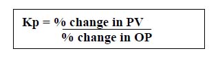
Because there is a control valve involved you cannot be sure that the process gain will be the same at all flow rates through the system. Therefore the value of Kp should be tested at different flow rates.
Carry out the following gain test in 20% increments starting at OP=10%
- Record PV(10) when OP = 10%
- Increase OP to 30% and allow the PV to stabilize
- Record PV (30) when OP = 30%
- Calculate Kp from the above equation.
- Repeat steps 1 to 4 for (30% to 50%) and (50% to 70%).
Remember to change the value of PV from the engineering scale of 300m3/hr to the percentage of full scale value
You should find that the gain Kp is reasonably constant = 1.5 over the range of operation. Very often this is not the case of course, particularly at the low and high ends of the control valve opening but for the moment we have set up an approximately linear relationship between 0 and 300m3/hr.
Now find the time constant of the first order lag in the process (process includes the valve). You can do this by repeating the step response from 30% to 60% OP in Manual and observing the time trace.

Finding the time constant of the first order lag
The lag is found by measuring the time from the initial movement of the PV until the PV reaches 62.3% of the new steady state value. Once you have most of the curve on screen press the PAUSE button and use the cursor on the trend display to read off the PV and time values. Record the original PV as PV1 and the new steady state value of PV as PV2. Then calculate the target PV point for the time constant as:
PVtc = PV1 + 62.3% (PV2 – PV1).
In the standard example you should be able to show that the time constant is 5.0 seconds as shown in Figure D1.4. Note that the response curve reaches approximately 99% of its final value after 4 time constants.
Changing parameters
The PC-Control Lab software allows you to inspect and change most parameters of the process being simulated. You should now experiment with changing and testing the gain and time constant values in the model by clicking on the command “ Process—Change Parameters”. Repeat the above the above tests to verify your chosen values.
Inserting dead time.
Caution: Dead time parameters in PC-Lab are stated in minutes. For example 0.1 minutes = 6seconds. Do not raise dead time above 1.0 minutes when operating in with the display grid set to SECONDS as this may cause corruption of the simulation. If this occurs simple reload PC-Lab.
Most processes exhibit some degree of dead time or “transport delay” in which the change in output to the process (more correctly the manipulated variable MV) has no effect at all on the PV until the change has had time to travel through a time period. (Opening the floodgates on a dam will not affect downstream residents until the surge has traveled to their neighborhood). In this simulation you may insert and observe the effect of dead time on a step change by increasing the parameter value from 0.01 to 1.0 or even higher. Figure D1.5 shows an example when dead time has been set to 6 seconds (0.1 minutes). This will make any a control loop much more difficult to stabilize so it should be restored to the minimum value of 0.01 before proceeding with the next stage of this practical.

Response to step change with dead time in the process
1.4 Open loop control
You can observe that without the advantage of automatic feedback from the PV your ability to drive the PV to a target value depends on knowing the gain of the process and zero offset or knowing what loading is placed on it.
Loading is the general term used in the simulation for an external disturbance on the process or for a measurement offset. The load on this particular process is the system pressure drop across the valve and flow meter. The normal pressure drop applies when the load parameter, displayed on the screen as a grey line, is at 50%. To observe the effect of a reduction in system pressure:
- Set the OP to 30% and allow the PV to stabilize, then just press the StepDecr button.
- Step the pressure down again until the grey line is on 40%. Observe that the flow falls each time as you might expect. The change in system pressure drop has changed the gain of the process
Now adjust the OP value to deliver PV = 180 m3/hr. Now increase the pressure drop by pressing the StepIncr button and observe the change in PV . Clearly , unless you know the exact amount of the disturbance you cannot easily restore the PV to 180 m3/hr unless you use feedback from the PV.
If the disturbance is caused by random noise in the process (in this case it could be a supply pressure deviation or a downstream pressure deviation) or in the measurement you will also not be able to maintain the PV at the target value by open loop control. For example: Insert noise by pressing the AutoLoad button and observe the random movement of the PV.
Conclusion for open loop control
Open loop control can only be used when the process characteristics are unchanging and undisturbed by external factors or if these factors can be accurately compensated out. In all other cases predicting the required output to achieve the desired PV will give poor results.
Exercise 4b
Flow Control Loop – Basic Example for Closed Loop Control
2.1 Objective
This exercise will familiarize the student with the basic concepts of closed loop control. It provides an opportunity to get a first feel for closed loop control and the open loop response of the process being controlled. A flow control loop as shown in Figure D2.1 will serve as a practical example for this exercise. A flow control loop is generally not difficult to operate and illustrates the basic principles effectively.

Basic Flow Control Loop
D2.2 Operation
This exercise follows directly from Exercise 1 in which you will have seen how to install and operate the PC ControLab simulation tool. Also in Exercise 1 you will have loaded the model IDC Flow1.mdl and tested its open loop response for gain and time constant. Make sure that you have completed these steps before proceeding with this exercise.
2.3 Operation in Auto mode
Prepare the model IDC Flow 1 for closed loop control by loading it from file folder Ex-2. Select the file location “PC-Pracs” and then subfolder “Ex-2” Highlight “IDC Flow 1.mdl “and press Open. Set the grid scale to seconds.
For some initial practice with the automatic control mode some suitable loop tuning values for controller gain and integral (reset) action must be loaded. Press the “Control” key on the toolbar and select the dropdown for “Retrieve strategy and tuning”. Select the file location to Ex-2, select: “IDC Flow Auto 1.stg” and open it. Now press the TUNE key and verify that you have Gain = 1.5 and Reset = 0.2 minutes per repeat.
The normal practice in setting a control loop to automatic is to first make sure that the set point (SP) is made equal to the present PV to avoid any disturbance as the automatic control action is started. Set point tracking has already been enabled in this strategy model so if you set the output to a starting value the set point will self-adjust to match the PV. Execute the following steps.
Step 1: Keep the controller in MAN and the display in RUN. Set OP = 20%.
Step 2: Note that the PV and SP settle at 45 m3/hr.
Step 3: Change the controller from MANUAL to AUTOMATIC mode.
Step 4: Change the set point to 210 m3/hr by using the SP button and typing in the new value.
Step 5: As soon you press OK you will see the response to this step change in the set point. You should obtain the response shown in Figure D2.2.

Basic flow loop auto response to step change in SP
2.4 Observation
As soon as the set point is changed the controller responds by driving the OUTPUT to reduce the error between SP and PV and the PV is steadily driven to the new Set Point. The controller tuning has been set up for proportional plus integral action control, hence you can see in Figure D2.2 that the proportional action brings the PV towards the SP but does not meet it until the integral action has increased the output over time until the error is zero.
2.5 Operation
You should now experiment on your own with changing the tuning parameters and repeating step changes to see the effect on the responses. The tuning parameters we are concerned with here are simple the controller gain and the integral action. Press TUNE on the display to access these parameters. If you want to get back to the settings used for the test run in Figure D2.2 simple reload the strategy file using the command CONTROL- RETRIEVE STRATEGY,MODEL and TUNING.
Since a flow control loop has no intrinsic stability problems, most effects can be observed clearly. You may also try introducing some dead time into the model as discussed in D2.3 above. Find how much dead time can be tolerated before the response becomes unstable.
This completes Exercises 1 and 2. By this stage you should be quite familiar with the basic features of the PC-Control Lab 3 facility.
Exercise 4c
Closed Loop Method – Tuning Exercise

3.1 Objective
This exercise will give some practical experience in the Closed Loop Tuning Method. It will show you how to recognize the characteristic responses shown by a close loop control system and how to use these features to guide you to find suitable PID tuning parameters.
We are going to use the exercise kindly provided by Wade Associates which involves an interactive step by step exercise in which you will record your answers on the question sheets.
Background: Tuning by closed loop process testing involves putting the controller in AUTOMATIC, removing all Reset and Derivative, and setting the Gain just high enough to cause a sustained process oscillation. From this test, the relevant parameters are the period of oscillation in minutes, and the Gain which ultimately caused the sustained oscillation. These are called the “ultimate Period” and “ultimate Gain”, respectively. From this data, the tuning parameters can be calculated.
Note: The open-loop (the subject of IDC Exercise 7) and the closed-loop methods (the closed-loop method is the subject of this exercise) may or may not produce similar tuning values, even when using the same process model. The “Generic” process model is used in these exercises; there is some difference in the results. For demonstration purposed, is you wish to obtain similar results from t he two methods, use the Generic2” model.
1. RUNNING THE PROGRAM
Start WINDOWS
Run PC-ControLAB
2. TUNING BY CLOSED LOOP PROCESS TESTS.
2.1 Setup
Confirm the following:
Process: GENERIC (see the top line, left hand side)
Select: Control Options/ Control Strategy: FEEDBACK (see the top line, right hand side)
Start PC-ControLAB
Select Control | Select Strategy | Feedback
Select Process | Select Model/ PC Pracs/EX-10/Generic.mdl
Select Process | Initialize to initialize the process model.
If you are more familiar with using Proportional Band, rather than Gain, for tuning controllers, or if you are more familiar with tuning the reset (integral) mode in Repeats per Minute, rather than Minutes per Repeat, then:
Press Tune then select the Options tab to set up the program to match the system you use:
Display GAIN as: Display RESET as:
GAIN Mins/Repeat
PROP BAND Repeats/Min
Press Tune then select the Options tab. Select Reset Action OFF.
2.2 Process Testing
| Set: | Gain: 1.0 or | PB:100% |
| Reset: | OFF (see above) | |
| Deriv: | 0.0 minutes |
Put the controller in Auto.
Make a set point change of 5% of full scale. (Press StepIncr once.)
If there is no oscillation, or if the oscillation dies out, increase the Gain (or decrease the Proportional Band) and repeat the set point change. (The Gain can initially be changed approximately 50% of its present value, or the PB can be changed to one-half of its present value. As the response gets closer to sustained oscillation, smaller changes should be made.) You should not have to observe the response for more than three cycles to determine whether or not the oscillation is decaying or not.)
When sustained oscillation is ultimately achieved, record the following:
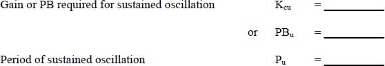
Use the table for the closed-loop Ziegler-Nichols method (Table 1 at the back of this exercise) to calculate tuning parameters for a P, PI and PID controller. Enter these in the table below:
(First calculate Gain (KC), Integral time (TI) and Derivative (TD) from the equations. Then, if your system uses PB rather than Gain, or Reset Rate rather than Reset Time, calculate those values.)
| P | PI | PID | |
|---|---|---|---|
| Gain (KC) | 4.5 | 4.0 | 5.4 |
| Prop Band (PB) | |||
| Integ Time (TI) (min/rpt) |
— | 5.8 | 3.5 |
| Reset Rate (rpt/min) |
— | — | |
| Deriv Time (TD) | — | — | 0.88 |
Before testing for the closed loop response, go to Tune | Options tab and set Reset Action ON.
For each type of controller, enter the parameters, put the controller in Auto and test the loop for a 10% (of full scale) set point change.
Calculate or measure the decay ratio, period and (for PI controller only) the period-to-integral time ratio. (This will be used in a subsequent exercise.)
Also, for each type of controller, make a 5% load change. (Press StepIncr or StepDecr.) Mark which controller type has the best, and the worst, response to a load change.
| P | PI | PID | |
|---|---|---|---|
| Decay Ratio | 0.16 | ||
| Period, mins | 9.2 | ||
| Period Integral Time |
— | — | |
| Load change, best and worst response | Worst | Best |
Table 1
Ziegler-Nichols Tuning Parameter Correlation For
Closed Loop Process Data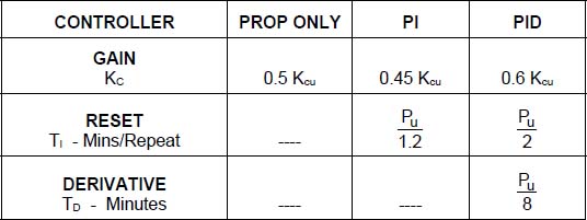
Kcu = Controller Gain that causes sustained oscillation
Pu = Period (in minutes) of sustained oscillation
= Time between any two successive peaks
Practical 5
Exercise in calculating CV for a liquid control valve
Question:
| Subject | Calculation of Cvs by application of sizing equations as applied to liquids |
| Objective | To developskills using the basic manual calculation method for Cv . This exercise is for individual participants |
| Relevance | The basis of all valve sizing work is to apply the relevant equations to calculate the valve capacity at various flowing consitions. Whilst computer tools are available for this knowing the fundamnetal methods allows the engineer to understanding the parameters involved in valve sizing . |
| Task detail | Two liquid sizing exercises are required. These are to be set down as set of cacluation steps based on the equations given in Chapter 3.The suggested approach is to set up a table containing the paramaters and calculated values for each step.
Task 1: Valve TV-1: Find the Cvs required for the flowing conditions given. Then from the table of valve data given select the most suitable sized valve for the job. Task 2: Valve FV-1: Find the Cvs required for the flowing conditions given. Then from the table of valve data given select the most suitable sized valve for the job. |
| Time Allowed | 45 minutes including time for discussion of answers. |
Task 1: Select a suitable size of control valve required for the performance requirements given below. Calculate the Cvs for the 3 flow rates given. Assume that a globe valve is to be used but using the range of valve sizes given select the most suitable body size for the valve.
| Valve tag | Line size-up | Line size-down | Type | Connection |
| TV-01 | 100 mm | 100 mm | Globe | 150 lb Flanged RF |
| Fluid | Max temp. | S.G at max temp | Vapour pressure Pv at max temp | Critical pressure Pc |
| Water | 80 C | .972 | 47.416 kPaA | 220.64 barA |
| Conditions | Max Flow | Normal | Min Flow | Units |
|---|---|---|---|---|
| Inlet Pressure | Inlet Pressure P1 | 800 | 850 | 900 |
| Outlet Pressure | Outlet Pressure P2 | 600 | 500 | 400 |
| Temperature | Temperature | 80 | 80 | 80 |
| Flow | Flow | 80 | 60 | 20 |
| Model | IDC-2 | IDC-3 | IDC-4 | IDC-6 |
| Body size | 50 | 80 | 100 | 150 |
| Max Cv | 46 | 110 | 195 | 400 |
| Cf (Fl) | .85 | .85 | 85 | .85 |
| Cfr (when D/d > 1.5) | .81 | .81 | .81 | .81 |
| Kc (incipient cavitation coefficient) | .58 | .58 | .58 | .58 |
Use the basic flow equations for liquid sizing as given in Chapter 3.
Task 2: Select a suitable size of control valve required for the performance requirements given below. Calculate the Cvs for the 3 flow rates given. Assume that a globe valve is to be used but using the range of valve sizes given select the most suitable body size for the valve.
| Valve tag | Line size-up | Line size-down | Type | Connection |
| FV-01 | 80 mm | 80 mm | Globe | 150 lb Flanged RF |
| Fluid | Max temp. | S.G at max temp | Vapour pressure Pv at max temp | Critical pressure Pc |
| Water | 90 C | .965 | 70.0 kPaA | 220.64 barA |
| Conditions | Max Flow | Normal | Min Flow | Units |
|---|---|---|---|---|
| Inlet Pressure | 400 | 450 | 500 | kPa(A) |
| Outlet Pressure | 300 | 250 | 150 | kPa(A) |
| Temperature | 90 | 90 | 90 | Deg C |
| Flow | 60 | 50 | 20 | m3/hr |
| Model | IDC-1.5 | IDC-2 | IDC-3 | IDC-4 |
| Body size | 40 | 50 | 80 | 100 |
| Max Cv | 25 | 46 | 110 | 195 |
| Cf (Fl) | .85 | .85 | .85 | 85 |
| Cfr (when D/d > 1.5) | .81 | .81 | .81 | .81 |
| Kc (incipient cavitation coefficient) | .58 | .58 | .58 | .58 |
Use the basic flow equations for liquid sizing as given in Chapter 3.
Answer:
Answer to task 1:
Using the basic flow equations for liquid sizing in metric units as given in Chapter 3.
The easiest way to set out the calculations is to make a table as shown below in which all the calculation steps can be recorded against each flow condition.
Step 1: Check for critical flow conditions: Find if ΔP>Cf2 (ΔPs)
The approximation for Δ Ps = P1 – Pv. Insert ΔP and Δ Ps in the table . Then insert Cf2 (ΔPs) and compare with ΔP. No chance of critical flow.
Step 2: for sub-critical flow use Cv = 1.16 q √ G f / Δ P inserted in the table and calculate the Cv
| Conditions | Max Flow | Normal | Min Flow | Units |
|---|---|---|---|---|
| Inlet Pressure P1 | 800 | 850 | 900 | kPa(A) |
| Outlet Pressure P2 | 600 | 500 | 400 | kPa(A) |
| Temperature | 80 | 80 | 80 | Deg C |
| Flow | 80 | 60 | 20 | m3/hr |
| Calc. ΔP in kPa | 200 | 350 | 500 | KPa |
| Calc ΔP in bar | 2 | 3.5 | 5 | Bar |
| Δ Ps = P1 – Pv. | 753 | 803 | 853 | KPa |
| Cf2 (ΔPs) | .852 x 753 = 544 | .852 x 853 = 580 | .852 x 1053 = 761 | |
| ΔP>Cf2 (ΔPs) Critical Flow? | No | No | No | |
| Calc Cv | 1.16 x 80 x (.972/ 2)1/2 | 1.16 x 60 x (.972 / 3.5)1/2 | 1.16 x 20 x (.972 / 5)1/2 | |
| 64.7 | 36.7 | 10.3 |
Step 3: Select the valve to provide the maximum required Cv when approximately 60% to 70 %of rated Cv. Minimum suggested rated Cv = 64.7/0.7 = 92
Step 4: Reference to the available valves in the question sheet indicates an 80 mm valve with Cv = 110.
This valve will be less than the line size of 100 mm so reducers will be needed. The flow capacity will be slightly reduced but for sub-critical flow the effect of the reduction where D/d is only 100/80 will be likely to be less than 5%. (based on data published in Masoneilan valve sizing manual).
N.B. Control valves are frequently sized below line size due to the much higher velocities permitted in the valve opening compared to the normal practice for pipelines.
Answer to task 2:
Using the basic flow equations for liquid sizing in metric units as given in Chapter 3.
Step 1: Check for critical flow conditions: Find if ΔP>Cf2 (ΔPs)
The approximation for Δ Ps = P1 – Pv. Insert ΔP and Δ Ps in the table. Then insert Cf2 (ΔPs) and compare with ΔP.
Critical flow occurs below the normal flow but above the minimum flow. If we are unable to change the flowing conditions we shall have to calculate the sizing based on the critical flow equations when dealing with the minimum flow condition.
Step 2: Cv = 1.16 q √ G f / Δ P for Max and Normal flows
For critical flow: Cv = 1.16q / Cf √ G f / Δ Ps and Δ Ps = P1 – Pv
| Conditions | Max Flow | Normal | Min Flow | Units |
|---|---|---|---|---|
| Inlet Pressure | 400 | 450 | 500 | kPa(A) |
| Outlet Pressure | 300 | 250 | 150 | kPa(A) |
| Temperature | 90 | 90 | 90 | Deg C |
| Flow | 60 | 50 | 20 | m3/hr |
| Calc. Δ P in kPa | 100 | 200 | 350 | kPa |
| Calc Δ P in bar | 1 | 2 | 3.5 | Bar |
| Δ Ps = P1 – Pv. (70.0) | 330 | 380 | 430 | kPa |
| Cf2 (ΔPs) | .852 x 330 = 238 | .852 x 380 = 275 | .852 x 430 = 311 | |
| ΔP>Cf2 (ΔPs) Critical Flow? | No | No | Yes | |
| Calc Cv | 1.16 x 60 x (.972/ 1)1/2 | 1.16 x 50 x (.972 / 2)1/2 | (1.16 x 20/0.85) x (.972 / 3.11)1/2 | |
| 68.6 | 40.4 | 12.2 |
Step 3: Select the valve to provide maximum required Cv when approximately 60% to 70 %of rated Cv. Minimum suggested rated Cv = 68.6/0.7 = 98
Step 4: Reference to the available valves in the question sheet indicates an 80 mm valve with Cv = 110.
This valve will be less than the line size of 100 mm so reducers will be needed. The flow capacity will be slightly reduced but for sub-critical flow the effect of the reduction where D/d is only 100/80 will be likely to be less than 5%. (Based on data published in Masoneilan valve sizing manual).
Practical 6
Exercise in calculating CV for a gas control valve
Question:
| Subject | Calculation of Cvs by application of sizing equations as applied to a valve to be used in flow control for a process using large volumes of compressed air. |
| Objective | To developskills using the basic manual calculation method for Cv . This exercise is for individual participants |
| Relevance | This is a typical air flow control problem. |
| Task detail | Task 1: For the valve FV-5: Find the Cvs required for the flowing conditions given. Then from the table of valve data given select the most suitable sized valve for the job.Task 2: When you have made your size selection check if reducers will be needed and try evaluating how much the Cv value for maximum flow will need to increase to compensate for the effect of reducers. Use the equation given in Chapter 4 for compensating for reducers. |
| Time Allowed | 30 minutes including time for discussion of answers. |
Task 1: Select a suitable size of control valve required for the performance requirements given below. Calculate the Cvs for the 3 flow rates given. Assume that a butterfly valve is to be used and select the most suitable body size for the valve using the range of valve sizes given Use the basic flow equations for liquid sizing as given in Chapter 4.
| Valve tag | Line size-up | Line size-down | Type | Connection |
| FV-05 | 200 mm | 200 mm | Butterfly | 150 lb Flanged RF |
| Fluid | Max temp. | S.G | ||
| Air | 50 C | 1 |
| Conditions | Max Flow | Normal | Min Flow | Units |
|---|---|---|---|---|
| Inlet Pressure | 1100 | 1000 | 900 | kPa(A) |
| Outlet Pressure | 800 | 800 | 800 | kPa(A) |
| Temperature | 80 | 80 | 80 | Deg C |
| Flow | 25000 | 20000 | 5000 | m3/hr |
| Model | IDC-3B | IDC-4B | IDC-6B | IDC –8B |
|---|---|---|---|---|
| Body size | 80 | 100 | 150 | 200 |
| Max Cv | 280 | 480 | 1330 | 2370 |
| Cf (Fl) | .65 | .65 | .65 | .65 |
| Cfr (when D/d > 1.5) | .6 | .6 | .6 | .6 |
Answer:
Answer to task 1:
Using the basic flow equations for gas sizing in metric units as given in Chapter 4.
Just as we established in P2 , the easiest way to set out the calculations is to make a table as shown below in which all the calculation steps can be recorded against each flow condition.
Step 1: Check for critical flow conditions: Find if ΔP> 0.50Cf2 P1
The critical condition is for sonic flow. From the table below it can be seen that this condition does not arise in this application..
Step 2: For sub-critical flow use Cv = (Q/295) √ GT / ( Δ P(P1+ P2). However because the flow is given in Normal m3/hr and the formula is based on a older USA convention of Standard m3/hr we have to correct the calculation for the difference in volumetric flow between these two reference values. The correction is to change temperature from 15 deg C to 0 deg c ( 288 K to 273K) and to change pressure from 101.3 kPa to 98.1 kPa.
So Q = Qn x (101.3/98.1) x ( 288/273) = 1.089 Qn
We then can modify the Cv formula as follows: Cv = (Qn/271) √ GT / ( Δ P(P1+ P2).
Using this version for volumetric flow when Qn = flow in Nm3/hr we can now tabulate the calculation just as was done for practical no 2.
| Conditions | Max Flow | Normal | Min Flow | Units |
|---|---|---|---|---|
| Inlet Pressure | 900 | 1000 | 1100 | kPa(A) |
| Outlet Pressure | 800 | 800 | 800 | kPa(A) |
| Temperature | 80 | 80 | 80 | Deg C |
| Flow Qn | 25000 | 20000 | 5000 | Nm3/hr |
| Calc. ΔP in kPa | 300 | 200 | 100 | kPa |
| Calc ΔP in bar | 1 | 2 | 3 | bar |
| 0.5Cf2 P1 | .5 x.652 x 300 = 63.4 | .5 x.652 x 200 = 42.2 | .5 x .652 x 100 = 21.1 | |
| ΔP> 0.5Cf2 P1 Critical Flow? | No | No | No | |
| Flow temperature T | 273+80 = 353 | 353 | 353 | Deg K |
| Calc Cv | (25000/271) x ((1 x 353)/1 x (9+8))1/2 | (20000/271) x ((1 x 353)/2 x (10+8))1/2 | (5000/271) x ((1 x 353)/3 x (11+8))1/2 | |
| 420.3 | 231.1 | 45.9 |
Step 3: Select the valve to provide the maximum required Cv when approximately 60% to 70 % of rated Cv. Minimum suggested rated Cv = 420.3/0.7 = 600
Step 4: Reference to the available valves in the question sheet indicates a 150 mm butterfly valve will be needed. This has a rated Cv = 1330. Whilst this may initially appear to be oversized it should be kept in mind that a butterfly valve flow characteristic is such that a fairly wide opening is required before Cvs rise to values above 50 % of rating.
We should also note that the 150 mm valve would require reducers to allow it to be fitted to a 200 mm line. Recall in Chapter 4 the reducer effect has the following formula:

Try inserting D = 200, d = 150, Cv = 420.3 to find R for the 150 mm valve at maximum flow. This is easiest to do on a spreadsheet. The value of R when Cv =420.3 is found to be: R = 0. 968. The reduction in Cv is therefore around 3%.
This means that we will need 3% more Cv in the valve to deliver the required Cv for the installed valve between reducers. The required Cv will rise to 434.
You can see that this result will not alter the valve selection but it is useful to see that the effect of reducers can be modeled. For more critical applications this correction may be significant.
Practical 7
Exercise in calculating CV for a steam control valve
Question:
| Subject | Calculation of Cvs by application of sizing equations as applied to a valve to be used in pressure control for a process using superheated steam |
| Objective | To developskills using the basic manual calculation method for Cv . This exercise is for individual participants |
| Relevance | This is a typical steam flow control problem. |
| Task detail | Task 1: For the valve PV-5: Find the Cvs required for the flowing conditions given. Then from the table of valve data given select the most suitable sized valve for the job. |
| Time Allowed | 30 minutes including time for discussion of answers. |
Task 1: Select a suitable size of control valve required for the performance requirements given below. Calculate the Cvs for the 3 flow rates given. Assume that a globe valve is to be used but using the range of valve sizes given select the most suitable body size for the valve.
| Valve tag | Line size-up | Line size-down | Type | Connection |
| PV-05 | 100 mm | 100 mm | Globe. Flow to close | 300 lb Flanged RF |
| Fluid | Temperature | Saturation temp at given pressures |
| Dry steam exiting from a superheater stage of a boiler | 400 C | |
| Pressure: 36 Bar a | 244.2 | |
| 34 Bar a | 240.9 | |
| 33 Bar a | 239.2 |
| Conditions | Max Flow | Normal | Min Flow | Units |
|---|---|---|---|---|
| Inlet Pressure | 33 | 34 | 36 | Bar a |
| Outlet Pressure | 30 | 30 | 30 | Bar a |
| Temperature | 400 | 400 | 400 | Deg C |
| Flow | 30000 | 25000 | 2000 | kg/hr |
| Model | 21000 | 21000 | 21000 | 21000 |
| Body size | 80 | 100 | 150 | 200 |
| Max Cv | 155 | 240 | 400 | 640 |
| Cf (Fl) | 0.94 | 0.94 | 0.92 | 0.92 |
| Cfr (when D/d > 1.5) | .87 | .87 | .87 | .87 |
Use the basic flow equations for dry steam sizing as given in Chapter 4.
Answer:
Answer to task 1:
This calculation uses the basic flow equations for steam flow valve sizing in metric units as given in Chapter 4.
Step 1: Decide which sizing equation is valid: Check for critical flow:
Is Δ P ≥ 0.5 Cf� P1?
Maximum Δ P = 5 bar
0.5 Cf� P1 = 0.5 x 0.92 x 0.92 x 33 = 13.9
So we can see that Δ P is much less than 0.5Cf� P1 and the flow regime is sub-critical. The transition to critical flow will occur if downstream pressure falls far enough to make Δ P greater than 13.9 bar. The equation to use for superheated steam is therefore:
For this calculation we need to know the degrees of superheat, Tsh. This value is easily obtained from steam tables and one very useful and convenient source for this data is the website: http://www.spiraxsarco.com/resources/steam-tables.asp. In this exercise we have already quoted the saturation temperature Tsat at the pressures we are using so you can alternatively obtain Tsh by subtracting Tsat from the steam temperature.
For 400 degree steam at the pressures we are using in this application the following Tsh values were returned:
| Steam pressure Bars absolute | Steam temperature Deg C | Tsh deg C | 1+0.00126Tsh |
| 36 | 400 | 155.8 | 1.196 |
| 34 | 400 | 159.0 | 1.200 |
| 33 | 400 | 160.7 | 1.202 |
The following results were obtained by creating a simple spreadsheet calculation table:
| Min Flow | Normal Flow | Max Flow | Units | |
|---|---|---|---|---|
| Inlet Pressure P1 | 36 | 34 | 33 | Bar a |
| Outlet Pressure P2 | 31 | 31 | 31 | Bar a |
| Pressure drop | 5 | 3 | 2 | Bar |
| Tsh | 155.8 | 159 | 160.7 | |
| 1+ .00126Tsh | 1.1963 | 1.2003 | 1.2025 | |
| Flow W | 2 | 20 | 30 | tons/hr |
| W ( 1+.00126Tsh) | 2.392616 | 24.0068 | 36.07446 | |
| DP ( P1 + P2) | 335 | 195 | 128 | |
| Sq root of above | 18.30 | 13.96 | 11.31 | |
| Cv = 72.4 x W()/above | 9.46 | 124.47 | 230.85 |
Valve Size Decision
The maximum Cv value obtained from the above calculation is compared with the Cvs of the available valves to find a valve that has a good margin of capacity above the maximum requirement. At the same time the valve must not be oversized since it is required to turndown its capacity to Cv = 9.46
Looking at the quoted Masoneilan 41000 series globe valves we find that the capacity values in the size range are as follows:
100mm size valve rated Cv = 195
150 mm size valve: rated Cv = 400
200 mm size valve : rated Cv = 640
Clearly the 100mm mm valve is too small and 200 mm valve is quite oversized. We conclude this case that the 150 mm valve would be a suitable choice. Because the application is for a pressure control task where the pressure drop does not change very much with the flow range it will be sensible to choose a linear characteristic. The percentage of rated Cv can be calculated as 230/400 = 57.5% . This will leave a good reserve for the boiler application in case where the boiler outlet pressure temporarily falls somewhat below 33 bar a.
Comparison with QuickSize results: When you have installed the Quicksize program as described in Chapter 5 you will be able to test this application on the software tool. Its is noticeable that the Quicksize program delivers the required Cv as 242.3 which is somewhat higher than this manual calculation. The reason for this is not apparent but it must be noted that the manual calculation is a basic tool that does not have the more complex correction factors used in computer calculations. In this case the deviation does not affect the decision in sizing.
Practical 8
Build a circuit, using 1 x NO (normally open) contact on each output, so that the light comes on each time the corresponding switch is flicked. (Please note that each switch operation may not result in a light switching on, if either the switch’s wires or the light’s wires have come loose, due to movement of the kit). However, most of the outputs should work correctly, and you will get the feel for your first successful project.
Practical 9
Keep the circuit almost exactly as it is, but change the bottom half of the contacts to NC (normally closed), as per Prac No 2 diagram. The idea, in this instance, is that the delegates can see how the PLC reads the altered inputs, and then inverts them before solving the logic.
Practical 10
Write a programme, so that any one of the switches, switches on all of the outputs. The actual idea of this prac is to see which switches and lamps work, and which do not. The delegate then marks these with a pen / tape, and avoids them for future exercises.
Practical 11
This practical really gets you to think. It takes a while, and there are three possible solutions.
Imagine there is a passage stairway, between two floors of a building. The passage has got one light bulb in the middle. On either floor, there is a switch, which operates the light. If you wish to move across the passage, and the light is of, flick the switch closest to you, in the opposite direction. When you get to the other end of the passage, and you wish to switch the light OFF, merely flick that switch to the opposite direction. Thus, from any side, you can switch the light on and off, at your own discretion. The idea is that you never have to walk in the passage, when it is dark. At the same time, you can switch off the passage light, to save electricity when not being used.
Just to help , the electrical diagram could be as follows:
Practical 12
With this practical, I would like to introduce the concept of motor control. You have a motor, which needs to be stopped and started. Use the top two (red) push buttons. The top button is for START, and the bottom is for STOP.
Practical 13
Here, I like to introduce you to counters. The idea is simple. Build an up-counter, and see how it works. NB – only build an up counter. A down counter, does not work well with this level of AB (Alan Bradley) PLC.
The task is simple. Build a counter, which will switch on a light, once a count of 5 is reached. Allow the counter to be reset.
Comments – see how the counter continues to count upwards, once the preset value is reached. (Some PLCs, such as Mitsubishi) stop accumulating, once this maximum value is reached.
To assign a timer, go to the left hand pane, double click on counters, and drag the full counter number (C5:0) to the counter in the PLC programme).
PS – when first loaded, you will only have one counter & one timer.
Double click on counter (in the left hand pane), click on properties. In the middle you will see:
LAST C5:0
Highlight this last number (i.e. the 0), and replace it with the number of counters you would like to have. Do the same, to increase timers at a later stage. The same applies, should you wish to increase the amount of bits (B’s).
To find the Counter-Done contact, double click on the counter pane (left hand side), and drag across the 0 directly under the DN letters. The same will apply to the timers, later on.
Practical 14
Here, I like to introduce you to timers. Build both timers at the same time, and compare their operations, by drawing a simple graph. The input is switched on, and the timer is checked, along with the corresponding light. Then the input is switched off, and the output is checked. You must play around with the time the switch is activated, to ensure all conditions are evaluated.
Notes
Remember to set the time base to 1.0!!!!!
With the On delay timer, the input must be closed for 5 seconds, before the light will switch on. As soon as the input falls away, the light goes off immediately.
With the Off delay timer, the light will illuminate, as soon as the input us closed. However, when the input is removed, the light remains on for 5 seconds.
Practical 15
CITECT practical
Objective
For Citect Version 5 Edit 3 (PROJECT NEW)
The Citect practical is designed to introduce the Citect software. This is accomplished by helping you set up, design, and run a working SCADA system. The system when running will display a main menu with seven buttons labelled TANK, ALARM, HARDWARE, TRENDS, SUMMARY, DISABLED and SHUTDOWN. You will be able to push any of the buttons and view the appropriate pages. The TANK page will show a working tank filling device. You will be able to move a tank fill switch and the tank on the screen will show a graph of the new tank level. If the tank is over-filled or underfilled an alarm will show on the screen. You will be able to view and clear the alarms in the ALARM and SUMMARY pages. You will be able to view a graph of the levels versus time in the TREND page. The SHUTDOWN button can be pressed to exit out of the system. The DISABLED page is used to disable alarms.
Citect design information
The Citect package is setup in a page format. Each page has to be opened, defined, and saved to a project. The pages used in this practical are kept simple because of time constraints. The Citect graphics builder and project editor are used to either design the pages or set up the software or compile and run the project. The flow of the project will be as follows. (Note the software must be setup in the following order.)
Hint – If you have any problems press the F1 key on the keyboard. This will show you the help screen.
Opening a new project
Open a Citect by clicking on the Citect icon on the desktop. Click on file then new project.
Type new. If this name is already used then put in one of your choosing. The screen should appear as follows (Add in the name new). Then press OK.
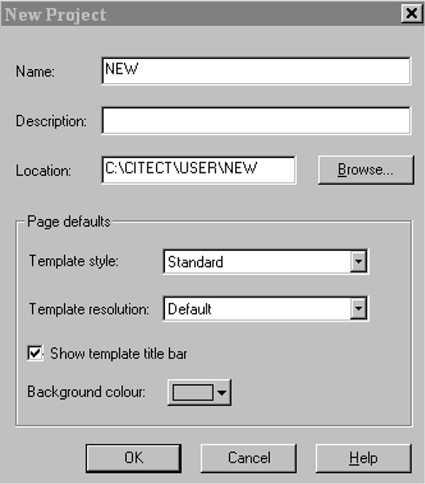
Do not press return. The ‘new’ project is now created.
Defining communications
Open the project editor by clicking on tools then project editor in the Citect explorer page.Define the type of communications by double clicking the express wizard in the communications menu. Follow the program to include the following selections;

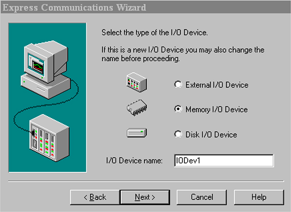
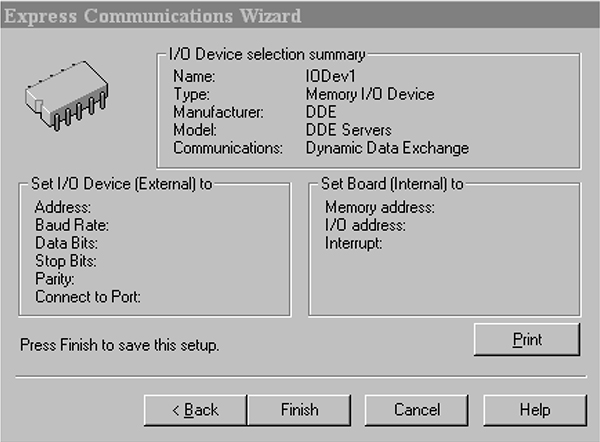
Defining tags
Go to the project editor. Click on tags on the menu. Setup your variable tag as shown and after the information is entered press add. Do not press return.
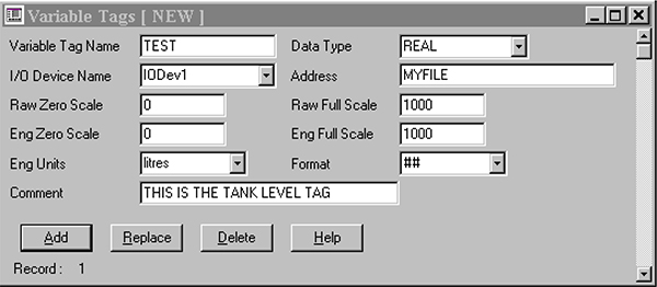
Trend tags
Still in the project editor, click on tags then trends tag on the menu. Setup your trends tag as shown and after the information is entered press add.
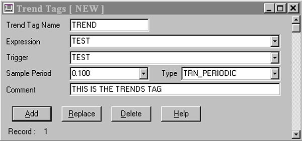
Analog alarm tags (found under alarms in the project editor)
There are four analogue alarm tags. These tags define the low, high, low low and high high alarms. The low alarm is set up for 250. The high alarm is set up for 750. The low low alarm is set for 100 and the high alarm is set for 900. Set up the four analogue alarms. Do this for all four alarms.
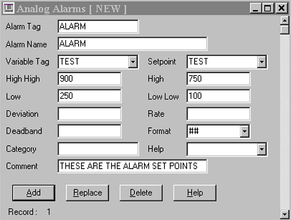
Creating the graphic pages

To change to the graphics builder click on tools then graphics builder. The graphic editor is used to add graphics pages to your project. You will create the pages (TANK, SUMMARY, DISABLED, ALARM, HARDWARE, TRENDS pages) in the graphics builder. Double click on new under the file menu. The screen should look like this:
Click on Page. The screen should change to:
Select the following pages and save them with the names provided. After opening each page, save and name each page with the following names.
ALARM – ALARM
HARDWARE – HARDWARE
NORMAL – TANK
SINGLE TREND – TRENDS
DISABLED – DISABLED
SUMMARY – SUMMARY
The only pages that need to be modified are the tank and trends pages. When all pages have been created and saved, open the tank page.
Building the tank page
The tank page will look like this when it is done.
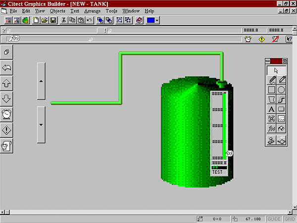
Use the paint menu on the right side of the page to select the switch and tank graph. Click on the small lamp icon and setup the switch as shown in the next picture.
Set up the tank by clicking on the small rubber stamp icon as shown in the next picture.
Set up the panel on the tank by selecting the panel under the lamp icon.
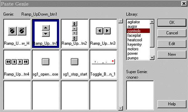
Selecting the trends page
Double click anywhere on the trends page, and the screen should come up as shown.
Double click again the trends page and the following page will come up. Set up as shown.

Compiling and running the project
Click on file at the top of the page and then again on compile. When the project has compiled click on file and then run.
When the program is running click on the switches and notice the tank graph will fill or empty. Notice the alarm at the top of the screen. Click on the flashing clock to view the alarm text. Click on the text and the alarm will be cancelled. To view the trends select the trends page.
Click and hold the tank button while moving the button up and down. Notice that the graph moves and if the level is over or under limits, the alarm will show up on the top of the screen. View the alarms by clicking on the flashing alarm clock on the top right of the screen. Also, view the trends by going back to the main menu and clicking on trends.
Practical 16
Configure SCADA Master Communications
Overview
This exercise will review the basic steps in configuring a SCADA master package to communicate with a MODBUS slave .
Hardware required
Two PCs with serial ports or USB to Serial adapters
Null modem cable
Software required
Citect Version 5.40.00 Service Pack C
Modbus Slave V3.10
Implementation
1. Setup SCADA master
Start Citect Explorer , Select Example Project then go to File menu and Copy Project to ..Copy Example project to New project called Modbus.
Select OK to copy project.
Go to Project Editor and open the Modbus project, then setup the device communication for Modbus as follows:
Note that some of the screens are not shown here. In most cases you can use the default values, but if unsure then consult the instructor.
Define the type of communications by double clicking the Express Wizard in the ‘Communications’ menu. Follow the program to include the following selections:

Select Add New I/O Device as we need to create a new communications link using the Modbus Protocol. Accept the I/O device name IODev. Click on An External I/O Device.
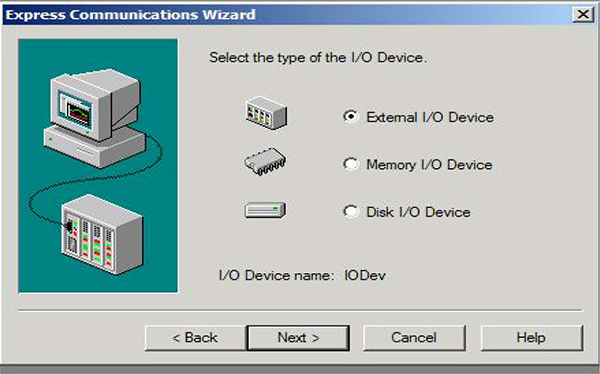
Choose Protocols. Select Modicon and then select Modicon then 484 and Serial (Modbus Binary Protocol)
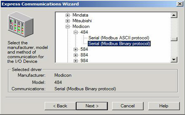
and Accept the Address. Select the serial COM Port to be used on the Computer ( in this case COM4). Finally select Save Changes and Close.
When the I/O device parameters are displayed hit Enter to confirm the default settings. These would be Address 1/ Baud Rate 19200/ Data Bits 8/ Stop Bits 1/ Even_P/
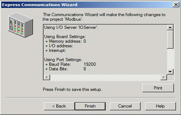
Confirm the settings by selecting Communication and reviewing each of the settings under Boards, Ports and I/O Devices. Under Ports modify the parameters to 9600baud/ 8 data bits/ 1stop bit/ no parity.
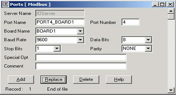
And Replace this record to modify the default setting
2. Modify analogue point in SCADA database
Select Tags and Variable Tags and scroll down to record 60 Loop_2_SP variable tag
Select the down arrow next to I/O Device Name and select IODev (as configured with Express Wizard). Modify the address to 30001. Observe the scales for the
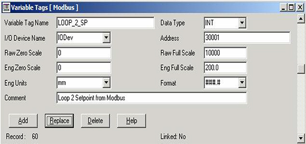
engineering units and the difference between raw full scale (which refers to the actual register values 0-10000) and Eng Full Scale (which refers to the real world engineering units 0-200mm).
Select Replace. The original record is now replaced. Close this window then Select File and Pack to consolidate all records.
The new configuration must now be compiled. Select Compile the Project. Once the compilation has successfully completed then select Run. As the program starts the following error will appear.

This is normal and click OK to run in Demo Mode.
Now go to the Loops Page and observe the Loop_2 details as follows:
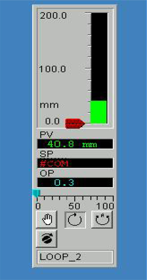
Note that the SP tag shows #COM which indicates a communication Error.
3. Setup Modbus slave
On another PC start Modbus Slave. Go to Setup, then Slave Definition and set Function 04 Address 1 Length 10 as shown. Note the display changes to addresses 30001- 30010.
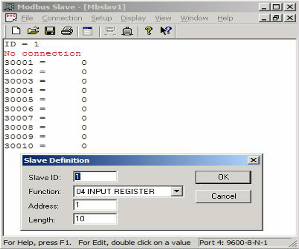
Go to Connection, then Connect and setup communication for the modbus simulator serial port Port 1 (if using COM1) , RTU mode and the same settings as the Master (9600 baud, 8 data bits, 1stop and No Parity.
4. Connect to Citect master
Connect a null modem cable between Modbus slave simulator and Citect Master COM4. Go to Display , Communications and observe the Modbus messages on the Slave.
You will notice that Citect eventually starts communicating with the RTU, but it initially sends an 02 Function Code to read the RTU status. When this occurs change RTU Function to 02 (using Slave Definition menu) and then the Citect Master starts sending the 04 messages to read 30001!
Change Function back to 04 on Slave and proper communication begins.
Note the Citect Master will show Loop_2 SP as 0 once communication has started. The Modbus Slave simulator is sending 0 for setpoint and the Citect master will then adjust the Loop2_PV to 0
On Modbus Slave double click on 30001 and change it within the range 0-10000 and observe the values change on the Master.
Practical 17
Protocol Analysis
Overview
This exercise is a brief introduction to protocol analysis, using a high-quality freeware Ethernet analyser.
Hardware required
Existing network infrastructure
Software required
Latest version of “Wireshark” or ‘Ethereal’ (from www.ethereal.com) plus the capture engine ‘winpcap’ version 3.1 or later.
Implementation
Install Wireshark (or Ethereal). Now set up your machine to ping another machine repetitively, e.g. ping 192.168.0.1 –t.
Click on the Ethereal GUI, or click start->programs->Ethereal

The Ethereal control panel will appear.
Click capture->start and select the appropriate network interface (in this case a Netgear 411 card).
You may experiment with the other default settings, but for now leave them as they are. It is possible to set up rather complex filters to screen out unwanted packets, but in this exercise we will set up the display filters afterwards.
Click OK. Capturing will commence and you will be able to observe some statistics regarding the packets being captured.
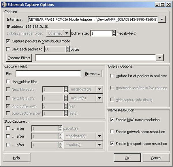
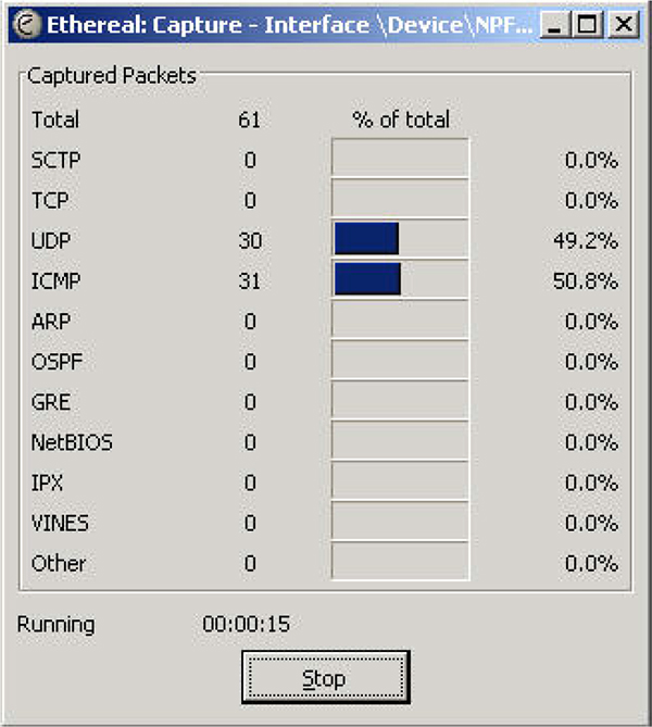
When you have captured a few ICMP packets, click stop and the captured packets will be displayed.
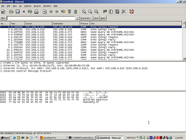
Now click analyze->display filters->expression?
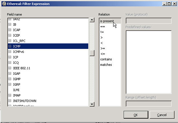
Select ‘+ICMP’ and ‘is present’, then click OK. Only the ping packets (ICMP) will now be displayed.
Highlight one of the echo request packets, then expand the Ethernet header (click on the ‘+’ next to ‘Ethernet’ ) in the middle screen.

Note the source and destination MAC addresses, with the first 6 characters decoded to show the manufacturer. In this case the destination is the D-Link DI-624 access point. Now expand the IP header.
Then the ICMP header.
In the bottom section of the screen you can observe the ICMP data (a, b, c, d, f, g, etc) embedded in the message.

Practical 18
Setting up Ethernet network
Overview
This exercise illustrates the setup of a very simple 10/100 Mbps Ethernet LAN. This will serve as the basis for our subsequent exercises.
Hardware required
The hardware required for this practical is as follows:
- Two or more laptops
- 1x Ethernet network interface card (NIC) per computer, unless the Ethernet interface is already built-in
- 1x Cat5 UTP fly-lead per computer
- 1 x hub. Note: the kit contains two small 5 port hubs (SureCom) that can be wired together if necessary.
Software required
The software required is as follows
- All the computers loaded with Windows 2000/XP
- Driver software for the NICs as provided by the manufacturer.
Implementation
To set up a basic network insert the NICs, if required, into the appropriate slots. Then connect each NIC to the hub with a flylead.
Hub connections
When the computer prompts you to log on, use the user name and password supplied by the instructor. You HAVE to log on if you require access to the LAN.
Now click Start -> Settings -> Control panel ->Network and Dial-up Connections. The red ‘X’ indicates that the NIC representing ‘local area connection 3’ is not currently connected to a hub.

Double-click the local area connection you wish to configure (e.g. local area connection 6 in this example). The following will appear:
Click on Properties.
Notice the following:
- The client (Client for Microsoft Networks) enables your computer to connect to other computers and access their resources
- ‘Connect using…..’ refers to the hardware device that physically connects your computer to the network, i.e. the Ethernet NIC in this case. The presence of the ‘adapter’ icon indicates that the driver for the card has been installed.
- The protocols occupying OSI layer 3 and 4 are, in our case, NetBEIU and TCP/IP. All hosts must use the same protocols in order to communicate with each other. Although TCP/IP would have been sufficient, NetBEUI had been added to facilitate file sharing between computers using NetBIOS names such as ‘computer1’. It will also allow you to access resources on the other machines in case TCP/IP is not working e.g. because of incorrect IP addresses.
- The service (File and Printer Sharing for Microsoft Networks) enables your computer to share its resources such as files, printers and other services with other computers on the network.
As soon as the NIC is inserted into the computer for the first time, the operating system prompts the user to provide the necessary device drivers. Thus the Client, Service, Adapter and Protocol components are automatically installed. TCP/IP is normally installed by default. If NetBEUI is not installed, you may have a problem seeing all the interconnected machines under ‘My Network Places’. You can add it with the ‘Install’ button just below the list of checked components.
Click OK and Close.
Now right click on My Computer, and then click on Properties and select Network Identification.

Now click on Properties and check/edit the computer name as well as the workgroup or domain name.
Computer name is a unique identity for your host computer on the network e.g. ‘Computer1’ (check with the instructor). This is also referred to as the NetBIOS name.
Workgroup is the name of the workgroup in which the host computer will appear e.g. ‘idc’ (check with the instructor). In the snag above, the workgroup name is shown as ‘domain’ but only because that was the name of the workgroup at that given moment in time; it does not refer to an actual domain.
You will be prompted for a user name and a password after rebooting. ALWAYS log on otherwise you will not get access to the network.
The computer should now be suitably configured for networking, and you can explore some troubleshooting of the wiring and hubs.
You will notice that the NIC and associated port on the hub both have their link integrity lights illuminated. Unplug the UTP cable and observe both lights extinguish. The link integrity lights are illuminated only when both devices are operational and correctly wired.
Unplug the UTP cable at both the NIC and hub and replace it with the crossover cable. Note that both sets of lights are extinguished because the wiring is now incorrect. If the hub has a crossover (Uplink) port then plug the crossover cable into this and observe the link integrity lights illuminate as the wiring is once again correct.
Plug the crossover cable directly into another NIC and observe both sets of lights illuminate. This is a useful way of connecting two computers without a hub, for file transfers etc.
If the link integrity light at the hub is not illuminated simply swap that cable to another working port on the hub to check that the port itself is not faulty.
Whenever data is being sent on the network the network activity lights on ALL ports and NICs will flicker since all messages on an Ethernet network are sent to all users. As other computers are being booted up onto the network activity should be noted. (NB: This is true for a hub, but not for a switch).
Some of the newer devices such as access points we will be using have auto MDIX on all or some ports, meaning that you can use either straight or crossover cable and the port will automatically configure itself.
Invoke Windows (e.g. right click on Start, then click Explore).
Select the C drive and then using the right mouse button right click on the same and select Sharing.
Select Share this folder and provide a share name for this resource. Click on Permissions to set access permissions. Click on Apply followed by OK.
Notice the small hand symbol under the C drive icon indicating that this drive is now shared.
Other resources may similarly be shared.
This concludes the basic network setup of host computers. To verify whether the network setup is OK, double click on My network places and Computers near me to view the other computers on the network. To see the shared resources available on a specific computer, just click its icon.
You may now browse the network neighborhood and the other computers’ shared resources. You may also transfer files back and forth across the network, view a remote file, execute a remote program, etc., all from the comfort of the local host computer.
Notes:
During boot-up, there may be errors displayed stating that there is already another computer on the network with the same name, and all networking services would be disabled. Follow the procedure described above and choose another computer name and restart
Some users may not be able to browse the network neighborhood (‘My network places’) since they have not logged in with an appropriate username and password at the time of boot-up. Log-off and logon as a valid user.
Others may not be able to either see their own host computer or one or more of the other host computers. This may be a result of not sharing any resources. Follow the procedure described above and share some resource, such as a folder.

Professional Certificate of Competency in Advanced TCP/IP-Based Industrial Networking
Designed for engineers and technicians who need practical knowledge in…Read more
Professional Certificate of Competency in Allen Bradley Controllogix / Logix5000 PLC Platforms
Designed for engineers and technicians who need practical knowledge in…Read more
Professional Certificate of Competency in Arc Flash Protection
Designed for engineers and technicians who work in the electrical…Read more
Professional Certificate of Competency in Chemical Engineering and Plant Design
Designed for engineers and technicians who need practical knowledge in…Read more
Professional Certificate of Competency in Circuit Breakers, Switchgear and Power Transformers
Designed for engineers and technicians who need practical knowledge regarding…Read more
Professional Certificate of Competency in Control Valve Sizing, Selection and Maintenance
Designed for engineers and technicians who need a solid understanding…Read more
Professional Certificate of Competency in Electrical Power System Fundamentals for Non Electrical Engineers
Designed for engineers and technicians who need to understand the…Read more
Professional Certificate of Competency in Electrical Power System Protection
Designed for engineers and technicians who need practical skills and…Read more")
Professional Certificate of Competency in Electrical Wiring Standards: AS/NZS 3000:2018 (Australia and New Zealand Only)
This professional development course is designed for engineers and technicians…Read more
Professional Certificate of Competency in Fundamental E & I Engineering for Oil and Gas Facilities
Designed for engineers and technicians who need to update their…Read more
Professional Certificate of Competency in Gas Turbine Engineering
Designed for engineers and technicians who need practical skills in…Read more
Professional Certificate of Competency in Hazardous Areas and Intrinsic Safety For Engineers and Technicians
Designed for engineers and technicians who need to understand the…Read more")
Professional Certificate of Competency in Heating, Ventilation and Air-Conditioning (HVAC)
Designed for engineers and technicians from a wide range of…Read more
Professional Certificate of Competency in IEC 61850 Based Substation Automation
Designed for engineers and technicians who need to understand the…Read more
Professional Certificate of Competency in Industrial Data Communications
Designed for engineers and technicians who need to understand how…Read more
Professional Certificate of Competency in Instrumentation, Automation and Process Control
Designed for engineers and technicians who need to gain practical…Read more
Professional Certificate of Competency in Machine Learning and Artificial Intelligence
This professional development course is designed for engineers and technicians…Read more
Professional Certificate of Competency in Mechanical Engineering
This professional development course is designed for engineers and technicians…Read more
Professional Certificate of Competency in Onshore and Offshore Pipeline Systems
Designed for engineers and technicians who need to gain an…Read more
Professional Certificate of Competency in Power Distribution
designed for engineers and technicians who need to gain a…Read more
Professional Certificate of Competency in Practical Machine Learning Using Python for Engineers and Technicians
Designed to use Python Programming to work with machine learning…Read more
Professional Certificate of Competency in Practical Python for Engineers and Technicians
Designed for engineers and technicians who need to understand the…Read more & SCADA Systems")
Professional Certificate of Competency in Programmable Logic Controllers (PLCs) & SCADA Systems
Designed for engineers and technicians who need to get practical…Read more
Professional Certificate of Competency in Project Management for Engineers & Technicians
This professional development course is designed for engineers and technicians…Read more
Professional Certificate of Competency in Safety Instrumentation Systems for Process Industries
Professional development course designed for engineers and technicians who want…Read more
Professional Certificate of Competency in Sewage and Effluent Treatment Technologies
Designed for engineers and technicians who need practical skills and…Read more
Professional Certificate of Competency in Structural Design for Non Structural Engineers
Professional development course designed for engineers and technicians who need…Read more")
Professional Certificate of Competency in Substation Design (Main Equipment)
Professional development course is designed for engineers and technicians who…Read more")
Professional Certificate of Competency in Substation Design (Control, Protection and Facility Planning)
Designed for engineers and technicians who need to gain practical…Read more
Professional Certificate of Competency in the Fundamentals of Process Plant Layout & Piping Design
Professional development course is designed for engineers and technicians who…Read more
Professional Certificate of Competency in Practical Mechanical Sealing
This professional development course is designed for engineers and technicians…Read more
Professional Certificate of Competency in Road Construction
This professional development course is designed for engineers and technicians…Read more
Professional Certificate of Competency in Specification and Technical Writing
Master the art of writing clear, accurate, and professional technical…Read more
Professional Certificate of Competency in Hydraulics and Pneumatics
Overview of all aspects related to the construction, design, operation,…Read more
Professional Certificate of Competency in Big Data and Analytics in Electricity Grids
This course explores the use of big data & data…Read more
Professional Certificate of Competency in Renewable Energy Systems
This course covers various renewable energy systems that are popular…Read more
Professional Certificate of Competency in Smart Grids
A smart grid is an electricity network that uses digital…Read more
Professional Certificate of Competency in Hydrogen Energy – Production, Delivery, Storage and Use
Hydrogen energy short course designed for engineers and professionals interested…Read more")
Professional Certificate of Competency in Building Information Modelling (BIM)
This professional development course is covering practical aspects of using…Read more
Professional Certificate of Competency in Industrial Internet of Things
Internet of Things (IoT) is the most sort after technology…Read more