")
52896WA Advanced Diploma of Civil and Structural Engineering (Materials Testing)
Investigation of the properties of construction materials, the principles which…Read more")
Graduate Diploma of Engineering (Safety, Risk and Reliability)
The Graduate Diploma of Engineering (Safety, Risk and Reliability) program…Read more
Professional Certificate of Competency in Fundamentals of Electric Vehicles
Learn the fundamentals of building an electric vehicle, the components…Read more
Professional Certificate of Competency in 5G Technology and Services Overview
Learn 5G network applications and uses, network overview and new…Read more
Professional Certificate of Competency in Clean Fuel Technology - Ultra Low Sulphur Fuels
Learn the fundamentals of Clean Fuel Technology - Ultra Low…Read more
Professional Certificate of Competency in Battery Energy Storage and Applications
Through a scientific and practical approach, the Battery Energy Storage…Read more
52910WA Graduate Certificate in Hydrogen Engineering and Management
Hydrogen has become a significant player in energy production and…Read more
Professional Certificate of Competency in Hydrogen Powered Vehicles
This course is designed for engineers and professionals who are…Read more
This manual covers the main aspects of TCP/IP and Ethernet in detail, including practical implementation, troubleshooting and maintenance.
Revision 6
Website: www.idc-online.com
E-mail: idc@idc-online.com
IDC Technologies Pty Ltd
PO Box 1093, West Perth, Western Australia 6872
Offices in Australia, New Zealand, Singapore, United Kingdom, Ireland, Malaysia, Poland, United States of America, Canada, South Africa and India
Copyright © IDC Technologies 2013. All rights reserved.
First published 2001
ISBN: 978-1-922062-07-9
All rights to this publication, associated software and workshop are reserved. No part of this publication may be reproduced, stored in a retrieval system or transmitted in any form or by any means electronic, mechanical, photocopying, recording or otherwise without the prior written permission of the publisher. All enquiries should be made to the publisher at the address above.
Disclaimer
Whilst all reasonable care has been taken to ensure that the descriptions, opinions, programs, listings, software and diagrams are accurate and workable, IDC Technologies do not accept any legal responsibility or liability to any person, organization or other entity for any direct loss, consequential loss or damage, however caused, that may be suffered as a result of the use of this publication or the associated workshop and software.
In case of any uncertainty, we recommend that you contact IDC Technologies for clarification or assistance.
Trademarks
All logos and trademarks belong to, and are copyrighted to, their companies respectively.
Acknowledgements
IDC Technologies expresses its sincere thanks to all those engineers and technicians on our training workshops who freely made available their expertise in preparing this manual.
Preface
One of the great protocols that has been inherited from the Internet is TCP/IP and this is being used as the open standard today for all network and communications systems. The reasons for this popularity are not hard to find. TCP/IP and Ethernet are truly open standards available to competing manufacturers and provide the user with a common standard for a variety of products from different vendors. In addition, the cost of TCP/IP and Ethernet is relatively low. Initially TCP/IP was used extensively in military applications and the purely commercial world such as banking, finance, and general business. But of great interest has been the strong movement to universal usage by the hitherto disinterested industrial and manufacturing spheres of activity who has traditionally used their own proprietary protocols and standards. These proprietary standards have been almost entirely replaced by the usage of the TCP/IP suite of protocols.
This is a hands-on book that has been structured to cover the main areas of TCP/IP and Ethernet in detail, while covering the practical implementation of TCP/IP in computer and industrial applications. Troubleshooting and maintenance of TCP/IP networks and communications systems in industrial environment will also be covered.
After reading this manual we would hope you would be able to:
- Understand the fundamentals of the TCP/IP suite of protocols
- Gain a practical understanding of the application of TCP/IP
- Learn how to construct a robust Local Area Network (LAN)
- Learn the basic skills in troubleshooting TCP/IP and LANs
- Apply the TCP/IP suite of protocols to both an office and industrial environment
Typical people who will find this book useful include:
- Network technicians
- Data communications managers
- Communication specialists
- IT support managers and personnel
- Network planners
- Programmers
- Design engineers
- Electrical engineers
- Instrumentation and control engineers
- System integrators
- System analysts
- Designers
- IT and MIS managers
- Network support staff
- Systems engineers
You should have a modicum of computer knowledge and know how to use the Microsoft Windows operating system in order to derive maximum benefit from this book.
The structure of the book is as follows.
Chapter 1: Introduction to Communications. This chapter gives a brief overview of what is covered in the book with an outline of the essentials of communications systems.
Chapter 2: Networking Fundamentals. An overview of network communication, types of networks, the OSI model, network topologies and media access methods.
Chapter 3: Half-duplex (CSMA/CD) Ethernet Networks. A description of the operation and performance of the older 10 Mbps Ethernet networks commencing with the basic principles.
Chapter 4: Fast and Gigabit Ethernet Systems. A minimum speed of 100 Mbps is becoming de rigeur on most Ethernet networks and this chapter examines the design and installation issues for Fast Ethernet and Gigabit Ethernet systems, which go well beyond the traditional 10 Mbps speed of operation.
Chapter 5: Introduction to TCP/IP. A brief review of the origins of TCP/IP to lay the foundation for the following chapters.
Chapter 6: Internet layer protocols. This chapter fleshes out the Internet Protocol (both IPv4 and IPv6) – perhaps the workhorses of the TCP/IP suite of protocols – and also examines the operation of ARP, RARP and ICMP.
Chapter 7: Host-to-Host (Transport) layer protocols. The TCP (Transmission Control Protocol) and UDP (User Datagram Protocol) are both covered in this chapter.
Chapter 8: Application layer protocols. A thorough coverage of the most important Application layer protocols such as FTP, TFTP, TELNET, DNS, WINS, SNMP, SMTP, POP, BOOTP and DHCP.
Chapter 9: TCP/IP utilities. A coverage focusing on the practical application of the main utilities such as PING, ARP, NETSTAT NBTSTAT, IPCONFIG, WINIPCFG, TRACERT, ROUTE and the HOSTS file.
Chapter 10: LAN system components. A discussion on the key components for interconnecting networks such as repeaters, bridges, switches and routers.
Chapter 11: VLANs. An overview of Virtual LANS; what they are used for, how they are set up, and how they operate.
Chapter 12: VPNs. This chapter discusses the rationale behind VPN deployment and takes a look at the various protocols and security mechanisms employed.
Chapter 13: The Internet for communication. The various TCP/IP protocols used for VoIP (Voice over IP) are discussed here, as well as the H.323 protocols and terminology.
Chapter 14: Security considerations. The security problem and methods of controlling access to a network will be examined in this chapter. This is a growing area of importance due to the proliferation attacks on computer networks by external parties.
Chapter 15: Process automation. The legacy architectures and the factory of the future will be examined here together with an outline of the key elements of the modern Ethernet and TCP/IP architecture.
Chapter 16: Troubleshooting Ethernet. Various troubleshooting techniques as well as the required equipment used will be described here, focusing on the medium as well as layers 1 and 2 of the OSI model.
Chapter 17: Troubleshooting TCP/IP. This chapter covers the troubleshooting and maintenance of a TCP/IP network, focusing on layers 3 and 4 of the OSI model and dealing with the use of protocol analyzers.
Chapter 18: Satellites and TCP/IP. An overview of satellites and the problems/solutions associated with running TCP/IP over a satellite link.
Learning objectives
When you have completed study of this chapter you should:
- Understand the main elements of the data communication process
- Understand the difference between analog and digital transmission
- Explain how data transfer is affected by attenuation, bandwidth and noise in the channel
- Comprehend the importance of synchronization of digital data systems
- Describe the basic synchronization concepts used with asynchronous and synchronous systems
- Explain the following types of encoding:
- Manchester
- RZ
- NRZ
- MLT-3
- 4B/5B
- Describe the basic error detection principles.
1.1 Data communications
Communications systems transfer messages from one location to another. The information component of a message is usually known as data (derived from the Latin word for items of information). All data is made up of unique code symbols or other entities on which the sender and receiver of the messages have agreed. For example, binary data is represented by two states viz. ‘0’ and ‘1’. These are referred to as binary digits or ‘bits’ and are represented inside computers by the level of the electrical signals within storage elements; a high level could represent a ‘1’, and a low-level could represent a ‘0’. Alternatively, the data may be represented by the presence or absence of light in an optical fiber cable.
1.2 Transmitters, receivers and communication channels
A communications process requires the following components:
- A source of the information
- A transmitter to convert the information into data signals compatible with the communications channel
- A communications channel
- A receiver to convert the data signals back into a form the destination can understand
- The destination of the information
This process is shown in Figure 1.1.

Communications process
The transmitter encodes the information into a suitable form to be transmitted over the communications channel. The communications channel moves this signal from the source to one or more destination receivers. The channel may convert this energy from one form to another, such as electrical to optical signals, whilst maintaining the integrity of the information so the recipient can understand the message sent by the transmitter.
For the communications to be successful the source and destination must use a mutually agreed method of conveying the data.
The main factors to be considered are:
- The form of signaling and the magnitude(s) of the signals to be used
- The type of communications link (twisted pair, coaxial, optic fiber, radio etc)
- The arrangement of signals to form character codes from which the message can be constructed
- The methods of controlling the flow of data
- The procedures for detecting and correcting errors in the transmission
The form of the physical connections is defined by interface standards. Some agreed-upon coding is applied to the message and the rules controlling the data flow and the detection and correction of errors are known as the protocol.
1.2.1 Interface standards
An interface standard defines the electrical and mechanical aspects of the interface to allow the communications equipment from different manufacturers to interoperate.
A typical example is the TIA-232-F interface standard (commonly known as RS-232). This specifies the following three components:
- Electrical signal characteristics – defining the allowable voltage levels, grounding characteristics etc
- Mechanical characteristics – defining the connector arrangements and pin assignments
- Functional description of the interchange circuits – defining the function of the various data, timing and control signals used at the interface
It should be emphasized that the interface standard only defines the electrical and mechanical aspects of the interface between devices and does not define how data is transferred between them.
1.2.2 Coding
A wide variety of codes have been used for communications purposes. Early telegraph communications used Morse code with human operators as transmitter and receiver. The Baudot code introduced a constant 5-bit code length for use with mechanical telegraph transmitters and receivers. The commonly used codes for data communications today are the Extended Binary Coded Decimal Interchange Code (EBCIDIC) and the American Standard Code for Information Interchange (ASCII).
1.2.3 Protocols
A protocol is essential for defining the common message format and procedures for transferring data between all devices on the network. It includes the following important features:
- Initialization: Initializes the protocol parameters and commences the data transmission
- Framing and synchronization: Defines the start and end of the frame and how the receiver can synchronize to the data stream
- Flow control: Ensures that the receiver is able to advise the transmitter to regulate the data flow and ensure no data is lost.
- Line control: Used with half-duplex links to reverse the roles of transmitter and receiver and begin transmission in the other direction.
- Error control: Provides techniques to check the accuracy of the received data to identify transmission errors. These include block redundancy checks and cyclic redundancy checks
- Time out control: Procedures for transmitters to retry or abort transmission when acknowledgments are not received within agreed time limits
1.2.4 Some commonly used communications protocols
- X/ Y/ Z modem and Kermit for asynchronous file transmission
- Binary Synchronous Protocol (BSC), Synchronous Data Link Control (SDLC) or High-Level Data Link Control (HDLC) for synchronous transmissions
- Industrial protocols such as Modbus and DNP3
1.3 Types of communication channels
An analog communications channel conveys signals that change continuously in both frequency and amplitude. A typical example is a sine wave as illustrated in Figure 1.2. On the other hand, digital transmission employs a signal of which the amplitude varies between a few discrete states. An example is shown in Figure 1.3.

Analog signal
Digital signal
1.4 Communications channel properties
1.4.1 Signal attenuation
As the signal travels along a communications channel its amplitude decreases as the physical medium resists the flow of the signal energy. This effect is known as signal attenuation. With electrical signaling some materials such as copper are very efficient conductors of electrical energy. However, all conductors contain impurities that resist the movement of the electrons that constitute the electric current. The resistance of the conductors causes some of the electrical energy of the signal to be converted to heat as the signal progresses along the cable resulting in a continuous decrease in the electrical signal. The signal attenuation is measured in terms of signal loss per unit length of the cable, typically dB/km.
To allow for attenuation, a limit is set for the maximum length of the communications channel. This is to ensure that the attenuated signal arriving at the receiver is of sufficient amplitude to be reliably detected and correctly interpreted. If the channel is longer than this maximum specified length, repeaters must be used at intervals along the channel to restore the signal to acceptable levels.

Signal repeaters
Signal attenuation increases as the frequency increases. This causes distortion to practical signals containing a range of frequencies. This problem can be overcome by the use of amplifiers that amplify the higher frequencies by greater amounts.
1.4.2 Channel bandwidth
The quantity of information a channel can convey over a given period is determined by its ability to handle the rate of change of the signal, i.e. the signal frequency. The bandwidth of an analog channel is the difference between the highest and lowest frequencies that can be reliably transmitted over the channel. These frequencies are often defined as those at which the signal at the receiving end has fallen to half the power relative to the mid-band frequencies (referred to as the -3 dB points), in which case the bandwidth is known as the -3 dB bandwidth.

Channel bandwidth
Digital signals are made up of a large number of frequency components, but only those within the bandwidth of the channel will be able to be received. It follows that the larger the bandwidth of the channel, the higher the data transfer rate can be and more high frequency components of the digital signal can be transported, and so a more accurate reproduction of the transmitted signal can be received.

Effect of channel bandwidth on digital signal
The maximum data transfer rate (C) of the transmission channel can be determined from its bandwidth, by use of the following formula derived by Shannon.
C= 2B log2 M bps
Where:
B = bandwidth in hertz and M levels are used for each signaling element.
In the special case where only two levels, ‘ON’ and ‘OFF’ are used (binary), M = 2 and C = 2 B. For example, the maximum data transfer rate for a PSTN channel with 3200 hertz bandwidth carrying a binary signal would be 2 × 3200 = 6400 bps. The achievable data transfer rate would then be reduced by half because of the Nyquist rate. It is further reduced in practical situations because of the presence of noise on the channel to approximately 2400 bps unless some modulation system is used.
1.4.3 Noise
As the signals pass through a communications channel the atomic particles and molecules in the transmission medium vibrate and emit random electromagnetic signals as noise. The strength of the transmitted signal is normally large relative to the noise signal. However, as the signal travels through the channel and is attenuated, its level can approach that of the noise. When the wanted signal is not significantly higher than the background noise, the receiver cannot separate the data from the noise and communication errors occur.
An important parameter of the channel is the ratio of the power of the received signal (S) to the power of the noise signal (N). The ratio S/N is called the Signal to Noise ratio, normally expressed in decibels (dB).
S/N = 10 log10 (S/N) dB
Where signal and noise levels are expressed in watts, or
S/N = 20 log10 (S/N) dB
Where signal and noise levels are expressed in volts
A high signal to noise ratio means that the wanted signal power is high compared to the noise level, resulting in good quality signal reception
The theoretical maximum data transfer rate for a practical channel can be calculated using the Shannon-Hartley law, which states that:
C = B log2 (1+S/N) bps
Where:
C = data rate in bps
B = bandwidth of the channel in hertz
S = signal power in watts and
N = noise power in watts
It can be seen from this formula that increasing the bandwidth or increasing the S/N ratio will allow increases to the data rate, and that a relatively small increase in bandwidth is equivalent to a much greater increase in S/N ratio.
Digital transmission channels make use of higher bandwidths and digital repeaters or regenerators to regenerate the signals at regular intervals and maintain acceptable signal to noise ratios. The degraded signals received at the regenerator are detected, then retimed and retransmitted as nearly perfect replicas of the original digital signals, as shown in Figure 1.7. Provided the signal to noise ratios is maintained in each link, there is no accumulated noise on the signal, even when transmitted over thousands of kilometers.

Digital link
1.5 Data transmission modes
1.5.1 Direction of signal flow
Simplex
A simplex channel is unidirectional and allows data to flow in one direction only, as shown in Figure 1.8. Public radio broadcasting is an example of a simplex transmission. The radio station transmits the broadcast program, but does not receive any signals back from the receiver(s).

Simplex transmission
This has limited use for data transfer purposes, as we invariably require the flow of data in both directions to control the transfer process, acknowledge data etc.
Half-duplex
Half-duplex transmission allows simplex communication in both directions over a single channel, as shown in Figure 1.9. Here the transmitter at ‘A’ sends data to a receiver at ‘B’. A line turnaround procedure takes place whenever transmission is required in the opposite direction. Transmitter ‘B’ is then enabled and communicates with receiver ‘A’. The delay in the line turnaround reduces the available data throughput of the channel.

Half-duplex transmission
Full-duplex
A full-duplex channel gives simultaneous communications in both directions, as shown in Figure 1.10.
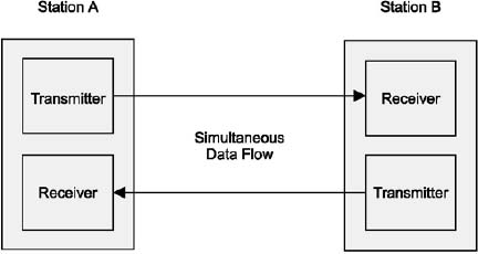
Full-duplex transmission
1.5.2 Synchronization of digital data signals
Data communications depends on the timing of the signal transmission and reception being kept correct throughout the message transmission. The receiver needs to look at the incoming data at correct instants before determining whether a ‘1’ or ‘0’ was transmitted. The process of selecting and maintaining these sampling times is called synchronization.
In order to synchronize their transmissions, the transmitting and receiving devices need to agree on the length of the code elements to be used, known as the bit time. The receiver also needs to synchronize its clock with that of the sender in order to determine the right times at which to sample the data bits in the message. A device at the receiving end of a digital channel can synchronize itself using either asynchronous or synchronous means as outlined below.
1.5.3 Asynchronous transmission
Here the transmitter and receiver operate independently, and the receiver synchronizes its clock with that of the transmitter (only) at the start of each message frame. Transmissions are typically around one byte in length, but can also be longer. Often (but not necessarily) there is no fixed relationship between one message frame and the next, such as a computer keyboard input with potentially long random pauses between keystrokes.

Asynchronous data transmission
At the receiver the channel is monitored for a change in voltage level. The leading edge of the start bit is used to set a bistable multivibrator (flip-flop), and half a bit period later the output of the flip-flop is compared (ANDed) with the incoming signal. If the start bit is still present, i.e. the flip-flop was set by a genuine start bit and not by a random noise pulse, the bit clocking mechanism is set in motion. In fixed-rate systems this half-bit delay can be generated with a monostable (one-shot) multivibrator, but in variable-rate systems it is easier to feed a 4-bit (binary or BCD) counter with a frequency equal to 16 times the data frequency and observing the ‘D’ (most significant bit) output, which changes from 0 to 1 at a count of eight, half-way through the bit period.

Clock synchronization at the receiver
The input signal is fed into a serial-in parallel-out shift register. The data bits are then captured by clocking the shift register at the data rate, in the middle of each bit. For an eight-bit serial transmission (data plus parity), this sampling is repeated for each of the eight data bits and a final sample is made during the ninth time interval to identify the stop bit and to confirm that the synchronization has been maintained to the end of the frame. Figure 1.13 illustrates the asynchronous data reception process.

Asynchronous data reception (clock too slow)
The receiver here is initially synchronized with the transmitter, and then maintains this synchronization throughout the continuous transmission of multiple bytes. This is achieved by special data coding schemes, such as Manchester, which ensure that the transmitted clock is encoded into the transmitted data stream. This enables the synchronization to be maintained at the receiver right to the last bit of the message, and thus allows larger frames of data (up to several thousand bytes) to be efficiently transferred at high data rates.
The synchronous system packs many bytes together and sends them as a continuous stream, called a frame. Each frame consists of a header, data field and checksum. Clock synchronization is provided by a predefined sequence of bits called a preamble.
In some cases the preamble is terminated with a ‘Start of Frame Delimiter’ or SFD. Some systems may append a post-amble if the receiver is not otherwise able to detect the end of the message. An example of a synchronous frame is shown in Figure 1.14. Understandably all high-speed data transfer systems utilize synchronous transmission systems to achieve fast, accurate transfers of large amounts of data.

Synchronous frame
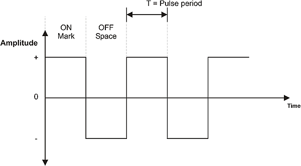
1.6 Encoding methods
1.6.1 Manchester
Manchester is a bi-phase signal-encoding scheme, and is used in the older 10 Mbps Ethernet LANs. The direction of the transition in mid-interval (negative to positive or positive to negative) indicates the value (‘1’ or ‘0’, respectively) and provides the clocking.
The Manchester codes have the advantage that they are self-clocking. Even a sequence of one thousand ‘0s’ will have a transition in every bit; hence the receiver will not lose synchronization. The price paid for this is a bandwidth requirement double that which is required by the RZ-type methods.
The Manchester scheme follows these rules:
- +V and –V voltage levels are used
- There is a transition from one to the other voltage level halfway through each bit interval
- There may or may not be a transition at the start of each bit interval, depending on whether the bit value is a ‘0’ or ‘1’
- For a ‘1’ bit, the transition is always from a –V to +V; for a ‘0’ bit, the transition is always from a +V to a –V
In Manchester encoding, the beginning of a bit interval is used merely to set the stage. The activity in the middle of each bit interval determines the bit value: upward transition for a ‘1’ bit, downward for a ‘0’ bit.
1.6.2 Differential Manchester
Differential Manchester is a bi-phase signal-encoding scheme used in Token Ring LANs. The presence or absence of a transition at the beginning of a bit interval indicates the value; the transition in mid-interval just provides the clocking.
For electrical signals, bit values will generally be represented by one of three possible voltage levels: positive (+V), zero (0 V), or negative (–V). Any two of these levels are needed – for example, + V and –V.
There is a transition in the middle of each bit interval. This makes the encoding method self-clocking, and helps avoid signal distortion due to DC signal components.
For one of the possible bit values but not the other, there will be a transition at the start of any given bit interval. For example, in a particular implementation, there may be a signal transition for a ‘1’ bit.
In differential Manchester encoding, the presence or absence of a transition at the beginning of the bit interval determines the bit value. In effect, ‘1’ bits produce vertical signal patterns; ‘0’ bits produce horizontal patterns. The transition in the middle of the interval is just for timing.
1.6.3 RZ (return to zero)
The RZ-type codes consume only half the bandwidth taken up by the Manchester codes. However, they are not self-clocking since a sequence of a thousand ‘0s’ will result in no movement on the transmission medium at all.
RZ is a bipolar signal-encoding scheme that uses transition coding to return the signal to a zero voltage during part of each bit interval. It is self-clocking.
In the differential version, the defining voltage (the voltage associated with the first half of the bit interval) changes for each ‘1’ bit, and remains unchanged for each ‘0’ bit.
In the non-differential version, the defining voltage changes only when the bit value changes, so that the same defining voltages are always associated with ‘0’ and ‘1’. For example, +5 volts may define a ‘1’, and –5 volts may define a ‘0’.
1.6.4 NRZ (non-return to zero)
NRZ is a bipolar encoding scheme. In the non-differential version it associates, for example, +5 V with ‘1’ and –5 V with ‘0’.
In the differential version, it changes voltages between bit intervals for ‘1’ values but not for ‘0’ values. This means that the encoding changes during a transmission. For example, ‘0’ may be a positive voltage during one part and a negative voltage during another part, depending on the last occurrence of a ‘1’. The presence or absence of a transition indicates a bit value, not the voltage level.
1.6.5 MLT-3
MLT-3 is a three-level encoding scheme that can also scramble data. This scheme is one proposed for use in FDDI networks. The MLT-3 signal-encoding scheme uses three voltage levels (including a zero level) and changes levels only when a ‘1’ occurs.
It follows these rules:
- +V, 0 V, and –V voltage levels are used
- The voltage remains the same during an entire bit interval; that is, there are no transitions in the middle of a bit interval
- The voltage level changes in succession; from +V to 0 V to –V to 0 V to +V, and so on
- The voltage level changes only for a ‘1’ bit
MLT-3 is not self-clocking, so that a synchronization sequence is needed to make sure the sender and receiver are using the same timing.
1.6.6 4B/5B
The Manchester codes, as used for 10 Mbps Ethernet, are self-clocking but consume unnecessary bandwidth (at 10 Mbps it introduces a 20 MHz frequency component on the medium). For this reason it is not possible to use it for 100 Mbps Ethernet, even over Cat5 cable. A solution is to revert back to one of the more bandwidth efficient methods such as NRZ or RZ. The problem with these, however, is that they are not self-clocking and hence the receiver loses synchronization if several zeros are transmitted sequentially. This problem, in turn, is overcome by using the 4B/5B technique.
The 4B/5B technique codes each group of four bits into a five-bit code. For example, the binary pattern 0110 is coded into the five-bit pattern 01110. This code table has been designed in such a way that no combination of data can ever be encoded with more than 3 zeros on a row. This allows the carriage of 100 Mbps data by transmitting at 125 MHz, as opposed to the 200 Mbps required by Manchester encoding.
 Table 1.1
4B/5B data coding
1.7 Error detection
All practical data communications channels are subject to noise, particularly where equipment is situated in industrial environments with high electrical noise, such as electromagnetic radiation from adjacent equipment or electromagnetic induction from adjacent cables. As a consequence the received data may contain errors. To ensure reliable data communication we need to check the accuracy of each message.
Asynchronous systems often use a single bit checksum, the parity bit, for each message, calculated from the seven or eight data bits in the message. Longer messages require more complex checksum calculations to be effective. For example the Longitudinal Redundancy Check (LRC) calculates an additional byte covering the content of the message (up to 15 bytes) while a two-byte arithmetic checksum can be used for messages up to 50 bytes in length. Most high-speed LANs use a 32-bit Cyclic Redundancy Check (CRC)
The CRC method detects errors with very high degree of accuracy in messages of any length and can, for example, detect the presence of a single bit error in a frame containing tens of thousands of bits of data. The CRC treats all the bits of the message block as one binary number that is then divided by a known polynomial. For a 32-bit CRC this is a specific 32-bit number, specially chosen to detect very high percentages of errors, including all error sequences of less than 32 bits. The remainder found after this division process is the CRC. Calculation of the CRC is carried out by the hardware in the transmission interface of LAN adapter cards.
Learning objectives
When you have completed study of this chapter you should be able to:
- Explain the difference between circuit switching and packet switching
- Explain the difference between connectionless and connection oriented communication
- Explain the difference between a datagram service and a virtual circuit
- List the differences between LANs, MANs and WANs
- Describe the concept of layered communications model
- Describe the functions of each layer in the OSI reference model
- Indicate the structure and relevance of the IEEE 802 Standards and Working Groups
- Identify hub, ring and bus topologies – from a physical as well as from a logical point of view
- Describe the basic mechanisms involved in contention, token passing and polling media access control methods
2.1 Overview
Linking computers and other devices together to share information is nothing new. The technology for Local Area Networks (LANs) was developed in the 1970s by minicomputer manufacturers to link widely separated user terminals to computers. This allowed the sharing of expensive peripheral equipment as well as data that may have previously existed in only one physical location.
A LAN is a communications path between two or more computers, file servers, terminals, workstations and various other intelligent peripheral equipment, generally referred to as devices or hosts. A LAN allows access to devices to be shared by several users, with full connectivity between all stations on the network. It is usually owned and administered by a private owner and is located within a localized group of buildings.
The connection of a device such as a PC or printer to a LAN is generally made through a Network Interface Card or NIC. The networked device is then referred to as a node. Each node is allocated a unique address and every message sent on the LAN to a specific node must contain the address of that node in its header. All nodes continuously watch for any messages sent to their own addresses on the network. LANs operate at relatively high speeds (Mbps range and upwards) with a shared transmission medium over a fairly small geographical (i.e. local) area.
On a LAN the software controlling the transfer of messages among the devices on the network must deal with the problem of sharing the common resources of the network without conflict or corruption of data. Since many users can access the network at the same time, some rules must be established by which devices can access the network, when, and under what conditions. These rules are covered under the general heading of Media Access Control.
When a node has access to the channel to transmit data, it sends the data within a packet (or frame) that generally includes, in its header, the addresses of both the source and the destination nodes. This allows each node to either receive or ignore data on the network.
2.2 Network communication
There are two basic types of communications processes for transferring data across networks, viz. circuit switching and packet switching. These are illustrated in Figure 2.1

Circuit switched and packet switched data
2.2.1 Circuit switching
In a circuit switched process a continuous connection is made across the network between the two different points. This is a temporary connection that remains in place as long as both parties wish to communicate, i.e. until the connection is terminated. All the network resources are available for the exclusive use of these two parties whether they are sending data or not. When the connection is terminated the network resources are released for other users. A call in an older (non-digital) telephone system is an example of a circuit switched connection.
The advantage of circuit switching is that the users have an exclusive channel available for the transfer of their data at any time while the connection is made. The obvious disadvantage is the cost of maintaining the connection when there is little or no data being transferred. Such connections can be very inefficient for the bursts of data that are typical of many computer applications.
2.2.2 Packet switching
Packet switching systems improve the efficiency of the transfer of bursts of data, by sharing the one communications channel with other similar users. This is analogous to the efficiencies of the mail system as discussed in the following paragraph.
When you send a letter by mail you post the stamped, addressed envelope containing the letter in your local mailbox. At regular intervals the mail company collects all the letters from your locality and takes them to a central sorting facility where the letters are sorted in accordance with the addresses of their destinations. All the letters for each destination are sent off in common mailbags to those locations, and are subsequently delivered in accordance with their addresses. Here we have economies of scale where many letters are carried at one time and are delivered by the one visit to your street/locality. Efficiency is more important than speed, and some delay is normal – within acceptable limits.
Packet switched messages are broken into a series of packets of certain maximum size, each containing the destination and source addresses and a packet sequence number. The packets are sent over a common communications channel, interleaved with those of other users. The ‘switches’ (routers) in the system forward the messages based on their destination address. Messages sent in multiple packets are reassembled in the correct order by the destination node.
All packets do not necessarily follow the same path. As they travel through the network they may get separated and handled independently from each other, but eventually arrive at their correct destination albeit out of their transmitted sequence. Some packets may even be held up temporarily (stored) at a node, due to unavailable lines or technical problems that might arise on the network. When the time is right, the node then allows the packet to pass or be ‘forwarded’.
The Internet is an example of a global packet switching network.
2.2.3 Datagrams and virtual circuits
Packet switched services generally support two types of services viz. datagram services and virtual circuits. In a self-contained LAN all packets will eventually reach their destination. However, if packets are to be switched ACROSS networks i.e. on an internetwork such as a Wide Area Network (WAN), then a routing decision must be made.
There are two possible approaches. The first is referred to as a ‘datagram’ service. The destination address incorporated in the data header will allow the routing to be performed. There is no guarantee when any packet will arrive at its destination, and sequential packets may well arrive out of sequence. The principle is similar to the mail service. You may send four postcards from your holiday in the South of France, but there is no guarantee that they will arrive in the same order that you posted them. If the recipient does not have a telephone, there is no easy method of determining that they have, in fact, been delivered.
Such a service is called an ’unreliable’ service. The term ‘unreliable’ is here not used in its everyday context, but instead refers to the fact that there is no mechanism for informing the sender whether the packet had been delivered or not. The service is also called ‘connectionless’ since there is no logical connection between sender and recipient.
The second approach is to set up a logical connection between transmitter and receiver, and to send packets of data along this connection or ‘virtual circuit’. Whilst this might seem to be in conflict with the earlier statements on circuit switching, it should be quite clear that this does NOT imply a permanent physical circuit being dedicated to the one packet stream of data. Instead, the circuit shares its capacity with other traffic. The important point to note is that the route for the data packets to follow is taken up-front when all the routing decisions are taken. The data packets just follow that pre-established route. This service is known as ‘reliable’ and is also referred to as a connection oriented service.
2.3 Types of networks
2.3.1 LANs
LANs are characterized by high-speed transmission over a restricted geographical area. Gigabit Ethernet (1000BaseX), for example, operates at 1000 Mbps. The restriction on size, though, is a deployment and cost issue and not a technical one, as current Ethernet technology allows switches to be interconnected with fiber into networks covering distances of thousands of kilometers.

Example of a LAN
2.3.2 WANs
While LANs operate where distances are relatively small, Wide Area Networks (WANs) are used to link LANs that are separated by large distances that range from a few tens of meters to thousands of kilometers. WANs normally use the public telecommunication system to provide cost-effective connection between LANs. Since these links are supplied by independent telecommunications utilities, they are commonly referred to (and illustrated as) a ‘communications cloud’. Routers perform this type of activity. They store the message at LAN speed and re-transmit it across the communications cloud at a different speed. When the entire message has been received at the access router of the remote LAN, it is once again forwarded at LAN speed. A typical speed at which a WAN interconnects varies between 9600 bps for a leased line to 40 Gbps for SDH/SONET. This concept is shown in Figure 2.3.

Example of a WAN
If reliability is needed for a time critical application, WANs can be considered quite unreliable, as delay in the information transmission is varied and wide. For this reason, WANs can only be used if the necessary error detection/correction software is in place, and if propagation delays can be tolerated within certain limits.
2.3.3 MANs
An intermediate type of network – a Metropolitan Area Network (MAN) – operates typically at 100Mbps. MANs use fiber optic technology to communicate over distances of up to several hundred kilometers. They are normally used by telecommunication service providers or utilities within or around cities. The distinction between MANs and LANs is, however, becoming rather academic since current Ethernet LAN technology (100 Mbps switches with 120 km fiber links) are also used to implement MANs.
2.3.4 Coupling ratio
The coupling ratio provides an academic yardstick for comparing the performance of these different kinds of networks. It is useful to give us an insight into the way these networks operate.
Coupling ratio α = τ / T
Where:
τ Propagation delay for packet
T Average packet transmission time
α = <<1 indicates a LAN
α = 1 indicates a MAN
α = >>1 indicates a WAN
This is illustrated in the following examples and Figure 2.4.
- 200 m LAN: With a propagation delay of about 1 mS, a 1000 byte packet takes about 0.8 ms to transmit at 10 Mbps. Therefore α is about 1 mS/0.8 ms or 1/800 which is very much less than 1. This means that for a LAN the packet quickly reaches the destination and the transmission of the packet then takes, say, hundreds of times longer to complete.
- 200 km MAN: With a propagation delay of about 1 mS, a 4000 byte packet takes about 0.4 ms to transmit at 100 Mbps. Therefore α is about 1 mS/0.4 ms or 2.4 which is reasonably close to 1. This means that for a MAN the packet reaches the destination and then may only take about the same time again to complete the transmission.
- 100 000 km WAN: With a propagation delay of about 0.5–2 seconds, a packet of 128 bytes takes about 10 ms to transmit at 1 Mbps. Therefore α is about 1 S/10 ms or 100. This means that for a WAN the packet reaches the destination after a delay of 100 times the packet length.

Coupling ratios
2.3.5 VPNs
A cheaper alternative to a WAN, which uses dedicated packet switched links (such as X.25) to interconnect two or more LANs, is the Virtual Private Network (VPN), which interconnects LANs by utilizing the existing Internet infrastructure.
A potential problem is the fact that the traffic between the networks shares all the other Internet traffic and hence all communications between the LANs are visible to the outside world. This problem is solved by utilizing encryption techniques to make all communications between the LANs transparent (i.e. illegible) to other Internet users.
2.4 The OSI model
A communication framework that has had a tremendous impact on the design of LANs is the Open Systems Interconnection (OSI) model. The objective of this model is to provide a framework for the coordination of standards development and allows both existing and evolving standards activities to be set within that common framework.
2.4.1 Open and closed systems
The wiring together of two or more devices with digital communication is the first step towards establishing a network. In addition to the hardware requirements as discussed above, the software problems of communication must also be overcome. Where all the devices on a network are from the same manufacturer, the hardware and software problems are usually easily overcome because all the system components have usually been designed within the same guidelines and specifications.
When devices from several manufacturers are used on the same application, the problems seem to multiply. Networks that are specific to one manufacturer and work with proprietary hardware connections and protocols are called closed systems. Usually these systems were developed at a time before standardization became popular, or when it was considered unlikely that equipment from other manufacturers would be included in the network.
In contrast, ‘open’ systems conform to specifications and guidelines that are ‘open’ to all. This allows equipment from any manufacturer that complies with that standard to be used interchangeably on the network. The benefits of open systems include wider availability of equipment, lower prices and easier integration with other components.
2.4.2 The OSI concept
Faced with the proliferation of closed network systems, the International Organization for Standardization (ISO) defined a ‘Reference Model for Communication between Open Systems’ (ISO 7498) in 1978. This has since become known as the OSI model. The OSI model is essentially a data communications management structure, which breaks data communications down into a manageable hierarchy (‘stack’) of seven layers. Each layer has a defined purpose and interfaces with the layers above it and below it. By laying down functions and services for each layer, some flexibility is allowed so that the system designers can develop protocols for each layer independently of each other. By conforming to the OSI standards, a system is able to communicate with any other compliant system, anywhere in the world.
The OSI model supports a client/server model and since there must be at least two nodes to communicate, each layer also appears to converse with its peer layer at the other end of the communication channel in a virtual (‘logical’) communication. The concept of isolation of the process of each layer, together with standardized interfaces and peer-to-peer virtual communication, are fundamental to the concepts developed in a layered model such as the OSI model. This concept is shown in Figure 2.5.

The OSI layering concept
The actual functions within each layer are provided by entities (abstract devices such as programs, functions, or protocols) that implement the services for a particular layer on a single machine. A layer may have more than one entity – for example a protocol entity and a management entity. Entities in adjacent layers interact through the common upper and lower boundaries by passing physical information through Service Access Points (SAPs). A SAP could be compared to a predefined ‘postbox’ where one layer would collect data from the previous layer. The relationship between layers, entities, functions and SAPs is shown in Figure 2.6.

Relationship between layers, entities, functions and SAPs
In the OSI model, the entity in the next higher layer is referred to as the N+1 entity and the entity in the next lower layer as N–1. The services available to the higher layers are the result of the services provided by all the lower layers.
The functions and capabilities expected at each layer are specified in the model. However, the model does not prescribe how this functionality should be implemented. The focus in the model is on the ‘interconnection’ and on the information that can be passed over this connection. The OSI model does not concern itself with the internal operations of the systems involved.
When the OSI model was being developed, a number of principles were used to determine exactly how many layers this communication model should encompass. These principles are:
- A layer should be created where a different level of abstraction is required
- Each layer should perform a well-defined function
- The function of each layer should be chosen with thought given to defining internationally standardized protocols
- The layer boundaries should be chosen to minimize the information flow across the boundaries
- The number of layers should be large enough that distinct functions need not be thrown together in the same layer out of necessity and small enough that the architecture does not become unwieldy
The use of these principles led to seven layers being defined, each of which has been given a name in accordance with its process purpose. The diagram below shows the seven layers of the OSI model.

The OSI reference model
The service provided by any layer is expressed in the form of a service primitive with the data to be transferred as a parameter. A service primitive is a fundamental service request made between protocols. For example, layer W may sit on top of layer X. If W wishes to invoke a service from X, it may issue a service primitive in the form of X.Connect.request to X. An example of a service primitive is shown in Figure 2.8. Service primitives are normally used to transfer data between processes within a node.

Service primitive
Typically, each layer in the transmitting site, with the exception of the lowest, adds header information, or Protocol Control Information (PCI), to the data before passing it through the interface between adjacent layers. This interface defines which primitive operations and services the lower layer offers to the upper one. The headers are used to establish the peer-to-peer sessions across the sites and some layer implementations use the headers to invoke functions and services at the N+1 or N–1 adjacent layers.
At the transmitter, the user application (e.g. the client) invokes the system by passing data, primitive names and control information to the highest layer of the protocol stack. The stack then passes the data down through the seven layers, adding headers (and possibly trailers), and invoking functions in accordance with the rules of the protocol at each layer. At each level, this combined data and header is called a Protocol Data Unit or PDU. At the receiving site, the opposite occurs with the headers being stripped from the data as it is passed up through the layers. These header and control messages invoke services and a peer-to-peer logical interaction of entities across the sites. Generally speaking, layers in the same stack communicate with parameters passed through primitives, and peer layers communicate with the use of the PCI (headers) across the network.
At this stage it should be quite clear that there is no physical connection or direct communication between the peer layers of the communicating applications. Instead, all physical communication is across the Physical, or lowest layer of the stack. Communication is down through the protocol stack on the transmitting node and up through the stack on the receiving node. Figure 2.9 shows the full architecture of the OSI model, whilst Figure 2.10 shows the effects of the addition of headers to the respective PDUs at each layer. The net effect of this extra information is to reduce the overall bandwidth of the communications channel, since some of the available bandwidth is used to pass control information.
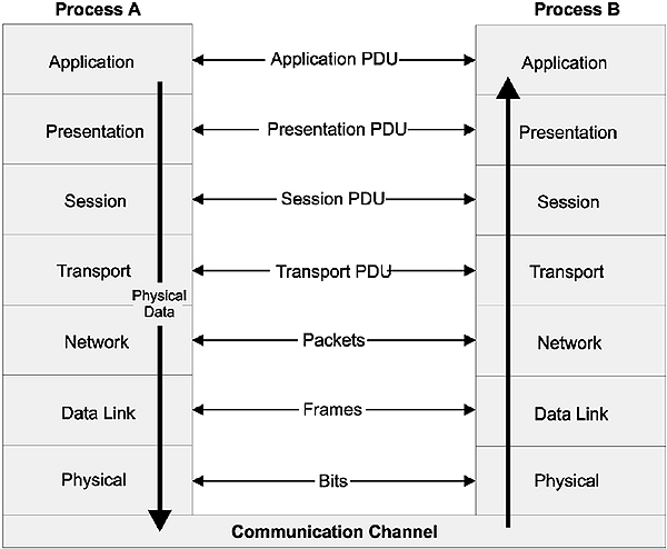
Full architecture of the OSI model
OSI message passing
2.4.3 OSI layer services
Briefly, the services provided at each layer of the stack are:
- Application
Provision of network services to the user’s application programs such as clients and servers. Note that the actual application programs do NOT reside here - Presentation
Maps the data representations into an external data format that will enable correct interpretation of the information on receipt. The mapping can also possibly include encryption and/or compression of data - Session
Control of the communications sessions between the users. This includes the grouping together of messages and the co-ordination of data transfer between grouped layers. It also inserts checkpoints for (transparent) recovery of aborted sessions - Transport
The management of the communications between the two end systems - Network
Responsible for the remote delivery of data packets. Functions include routing of data, network addressing, fragmentation of large packets, congestion and flow control. - Data Link
Responsible for sending a frame of data from one system to another. Attempts to ensure that errors in the received bit stream are not passed up into the rest of the protocol stack. Error correction and detection techniques are used here - Physical
Defines the electrical and mechanical connections at the physical level, or the communication channel itself. Functional responsibilities include modulation, multiplexing and signal generation.
The medium itself is not part of the Physical layer, although the Physical layer defines which medium is to be used. A more specific discussion of each layer is now presented.
2.4.4 Application layer
The Application layer is the topmost layer in the OSI reference model. This layer is responsible for giving applications access to the network. Examples of application-layer tasks include file transfer, electronic mail (e-mail) services, and network management. Application-layer services are much more varied than the services in lower layers, because the entire range of application and task possibilities is available here. The specific details depend on the framework or model being used. For example, there are several network management applications. Each of these provides services and functions specified in a different framework for network management. Programs can get access to the application-layer services through Application Service Elements (ASEs). There are a variety of such application service elements; each designed for a class of tasks. To accomplish its tasks, the application layer passes program requests and data to the presentation layer, which is responsible for encoding the Application layer’s data in the appropriate form.
2.4.5 Presentation layer
The Presentation layer is responsible for presenting information in a manner suitable for the applications or users dealing with the information. Functions such as data conversion from EBCDIC to ASCII (or vice versa), the use of special graphics or character sets, data compression or expansion, and data encryption or decryption are carried out at this layer. The Presentation layer provides services for the Application layer above it, and uses the Session layer below it. In practice, the presentation layer rarely appears in pure form, and it is the least well defined of the OSI layers. Application- or Session-layer programs will often encompass some or all of the Presentation layer functions.
2.4.6 Session layer
The Session layer is responsible for synchronizing and sequencing the dialog and packets in a network connection. This layer is also responsible for ensuring that the connection is maintained until the transmission is complete and that the appropriate security measures are taken during a ‘session’ (i.e., a connection). The Session layer is used by the Presentation layer above it, and uses the Transport layer below it.
Transport layer
In the OSI reference model, the Transport layer is responsible for providing data transfer at an agreed-upon level of quality, such as at specified transmission speeds and error rates. To ensure delivery, some Transport layer protocols assign sequence numbers to outgoing packets. The Transport layer at the receiving end checks the packet numbers to make sure all have been delivered and to put the packet contents into the proper sequence for the recipient. The Transport layer provides services for the session layer above it, and uses the Network layer below it to find a route between source and destination. The Transport layer is crucial in many ways, because it sits between the upper layers (which are strongly application-dependent) and the lower ones (which are network-based).
The layers below the Transport layer are collectively known as the ‘subnet’ layers. Depending on how well (or not) they perform their functions, the Transport layer has to interfere less (or more) in order to maintain a reliable connection.
2.4.7 Network layer
The Network layer is the third layer from the bottom up, or the uppermost ‘subnet layer’. It is responsible for the following tasks:
- Determining addresses or translating from hardware to network addresses. These addresses may be on a local network or they may refer to networks located elsewhere on an internetwork. One of the functions of the network layer is, in fact, to provide capabilities needed to communicate on an internetwork
- Finding a route between a source and a destination node or between two intermediate devices
- Fragmentation of large packets of data into frames small enough to be transmitted by the underlying Data Link layer through a process called fragmentation. The corresponding Network layer at the receiving node undertakes reassembly of the packet
2.4.8 Data Link layer
The Data Link layer is responsible for creating, transmitting, and receiving data packets. It provides services for the various protocols at the Network layer, and uses the Physical layer to transmit or receive material. The Data Link layer creates packets appropriate for the network architecture being used. Requests and data from the Network layer are part of the data in these packets (or frames, as they are often called at this layer). These packets are passed down to the Physical layer and from there they are transmitted to the Physical layer on the destination host via the medium. Network architectures (such as Ethernet, ARCnet, Token Ring, and FDDI) encompass the Data Link and Physical layers.
The IEEE 802 networking working groups have refined the Data Link layer into two sub-layers viz, the Logical Link Control (LLC) sub-layer at the top and the Media Access Control (MAC) sub-layer at the bottom. The LLC sub-layer provides an interface for the Network layer protocols, and control the logical communication with its peer at the receiving side. The MAC sub-layer controls physical access to the medium.
2.4.9 Physical layer
The Physical layer is the lowest layer in the OSI reference model. This layer gets data packets from the Data Link layer above it, and converts the contents of these packets into a series of electrical signals that represent ‘0’ and ‘1’ values in a digital transmission. These signals are sent across a transmission medium to the Physical layer at the receiving end. At the destination, the physical layer converts the electrical signals into a series of bit values. These values are grouped into packets and passed up to the Data Link layer.
The required mechanical and electrical properties of the transmission medium are defined at this level. These include:
- The type of cable and connectors used. Cable may be coaxial, twisted-pair, or fiber optic. The types of connectors depend on the type of cable
- The pin assignments for the cable and connectors. Pin assignments depend on the type of cable and also on the network architecture being used
- The format for the electrical signals. The encoding scheme used to signal ‘0’ and ‘1’ values in a digital transmission or particular values in an analog transmission depend on the network architecture being used
The medium itself is, however, not specific here. For example, Fast Ethernet dictates that Cat5 cable should be used, but the cable itself is specified in TIA/EIA-568B.
2.5 Interoperability and internetworking
Interoperability is the ability of network users to transfer information between different communications systems; irrespective of the way those systems are supported. One definition of interoperability is:
‘The capability of using similar devices from different manufacturers as effective replacements for each other without losing functionality or sacrificing the degree of integration with the host system. In other words, it is the capability of software and hardware systems on different devices to communicate together. This results in the user being able to choose the right devices for an application independent of the supplier, control system and the protocol.’
Internetworking is a term that is used to describe the interconnection of differing networks so that they retain their own status as a network. What is important in these concepts is that internetworking devices be made available so that the exclusivity of each of the linked networks is retained, but that the ability to share information, and physical resources if necessary, becomes both seamless and transparent to the end user.
At the plant floor level the requirement for all seven layers of the OSI model is often not required or appropriate. Hence a simplified OSI model is often preferred for industrial applications where time critical communications is more important than full communications functionality provided by the full seven layer model. Such a protocol stack is acceptable since there will be no internetworking at this level. A well-known stack is that of the S-50 Fieldbus standard, which is shown in Figure 2.11.
Generally most industrial protocols are written around the Data Link layer (to send/receive frames) and the Application layer (to deal with clients and servers). The Physical layer is required for access to the bus.
When the reduced OSI model is implemented the following limitations exist:
- The maximum size of the application messages is limited by the maximum size allowed on the channel, as there is no Network layer to fragment large packets
- No routing of messages is possible between different networks, as there is no Network layer
- Only half-duplex communications is possible, as there is no Session layer
- Message formats must be the same for all nodes (as there is no Presentation layer)
One of the challenges with the use of the OSI model is the concept of interoperability and the need for definition of another layer above the Application layer, called the ‘User’ layer. The user layer is not formally part of the OSI model but is found in systems such as DeviceNet, ProfiBus and Foundation Fieldbus to accommodate issues such as device profiles and software building blocks (‘function blocks’) for control.
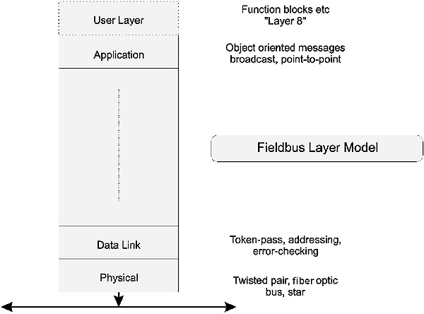
Reduced OSI stack
Most modern field buses no longer adhere to the 3 layer concept, and implement a full stack (including TCP/IP) in order to provide routing and hence allow large-scale deployment. Examples are ProfiNet, IDA and Ethernet/IP.
From the point of view of internetworking, TCP/IP operates as a set of programs that interacts at the transport and network layer levels without needing to know the details of the technologies used in the underlying layers. As a consequence this has developed as a de facto industrial internetworking standard. Many manufacturers of proprietary equipment are using TCP/IP to facilitate internetworking.
2.6 Protocols and protocol standards
A protocol has already been defined as the rules for exchanging data in a manner that is understandable to both the transmitter and the receiver. There must be a formal and agreed set of rules if the communication is to be successful. The rules generally relate to such responsibilities as error detection and correction methods, flow control methods, and voltage and current standards. However, there are other properties such as the size of the data packet that are important in the protocols that are used on LANs.
Another important responsibility is the method of routing the packet, once it has been assembled. In a self-contained LAN i.e. intranetwork, this is not a problem since all packets will eventually reach their destination by virtue of design. However, if the packet is to be switched across networks i.e. on an internetwork – such as a WAN – then a routing decision must be made. In this regard we have already examined the use of a datagram service vis à vis a virtual circuit.
In summary, there are many different types of protocols, but they can be classified in terms of their functional emphasis. One scheme of classification is:
- Master/slave vs peer-to-peer
A master/slave relationship requires that one of the communicators act as a master controller. Peer-to-peer protocols allow all communications to take place as and when required - Connection oriented
A connection-oriented protocol first establishes a logical connection with its counterpart before transmitting data. A connectionless protocol just sends the data regardless. - Asynchronous vs synchronous
Synchronous protocols send data in frames at the clock rate of the network. Asynchronous protocols send data one byte at a time, with a varying delay between each byte - Layered vs monolithic
The OSI model illustrates a layered approach to protocols. The monolithic approach uses a single layer to provide all functionality - Heavy vs light
A heavy protocol has a wide range of functions built in, and consequently incurs a high processing delay overhead. A light protocol incurs low processing delay but only provides minimal functionality
2.7 IEEE/ISO standards
The Institute of Electrical and Electronic Engineers in the USA has been given the task of developing standards for local area networking under the auspices of the IEEE 802 LAN/MAN Standards Committee (LMSC). Some IEEE LAN/MAN standards (but not all) are also ratified by the International Organization for Standardization and published as an ISO-IEC standard with an ‘8’ in front of the 802 designation. To date, the following LAN/MAN standards have been published by the ISO: ISO/IEC 8802.1, ISO/IEC 8802.2 ISO.IEC 8802.3, ISO/IEC 8802.5 and ISO/IEC 8802.11.
The LMSC assigns various topics to working groups and Technical Advisory Groups (TAGs). Some of them are listed below, but it must be kept in mind that it is an ever-changing situation.
2.7.1 IEEE 802.1 Bridging and Management
This sub-committee is concerned with issues such as high level interfaces, internetworking and addressing.
There are a series of sub-committees (thirteen at present), such as:
- 802.1B LAN/WAN management
- 802.1D MAC bridges
- 802.1E System Load Protocol
- 802.1F Common Definitions and Procedures for IEEE 802 Management Information
- 802.1G Remote MAC bridging
- 802.1X Port Based Network Access Control
2.7.2 IEEE 802.2 Logical Link Control
This is the interface between the Network layer and the specific network environments at the Physical layer. The IEEE has divided the Data Link layer in the OSI model into two sub-layers viz. the Media Access Control (MAC) sub-layer, and the Logical Link Control (LLC) sub-layer. The LLC protocol is common for most IEEE 802 standard network types. This provides a common interface to the network layer of the protocol stack. The IEEE 802.2 protocol used at this sub-layer is based on IBM’s HDLC protocol, and can be used in three modes.
These are:
- Type 1: Unacknowledged connectionless link service
- Type 2: Connection oriented link service
- Type 3: Acknowledged connectionless link service, used in real time applications such as manufacturing control
2.7.3 IEEE 802.3 CSMA/CD
The Carrier Sense, Multiple Accesses with Collision Detection type LAN is commonly, but strictly speaking incorrectly, known as Ethernet. Ethernet actually refers to the original DEC/INTEL/XEROX product known as Version II (Bluebook) Ethernet.
Subsequent to ratification this system has been known as IEEE 802.3. IEEE 802.3 is virtually, but not entirely, identical to Bluebook Ethernet. The frame contents differ marginally and the following chapter will deal with this anomaly.
Subsequently, several additional specifications have been approved such as IEEE 802.3u (100 Mbps or Fast Ethernet), IEEE 8023z (1000 Mbps or Gigabit Ethernet) and IEEE 802.3ae (10000 Mbps or Ten Gigabit Ethernet).
2.7.4 IEEE 802.5 Token Ring
This standard is the ratified version of the original IBM Token Ring LAN. In IEEE 802.5, data transmission can only occur when a station holds a token. The logical structure of the network wiring is in the form of a ring, and each message must cycle through each station connected to the ring.
The original specification called for a single ring, which creates a problem if the ring gets broken. A subsequent enhancement of the specification, IEEE 802.5u, introduced the concept of a dual redundant ring, which enables the system to continue operating in case of a cable break.
The original IBM Token Ring specification supported speeds of 4 and 16 Mbps. IEEE 802.5 at first supported only 1 and 4 Mbps, but currently includes 100 Mbps and 1 Gbps versions.
The physical media for Token Ring can be unshielded twisted pair, shielded twisted pair, coaxial cable or optical fiber.
2.7.5 IEEE 802.11 Wireless LANs
The IEEE 802.11 Wireless LAN standard uses the 2.4 GHz band and allows operation to 1 or 2 Mbps. The 802.11b standard also uses the 2.4 GHz band, but allows operation at 11 Mbps. The IEEE 802.11a specification uses the 5.7 GHz band instead and allows operation at 54 Mbps. The IEEE 802.11g specification allows operation at 54 Mbps using the 2.4 Ghz band. The next generation of products (IEEE 802.11n) will support 100 Mbps.
2.7.6 IEEE 802.12 Demand Priority Access
This specification covers the system known as 100VG AnyLAN. Developed by Hewlett-Packard, this system operates on voice grade (Cat3) cable – hence the VG in the name. The AnyLAN indicates that the system can interface with both IEEE 802.3 and IEEE 802.5 networks (by means of a special speed adaptation bridge).
Other working groups and TAGs include:
- IEEE 802.15 Wireless PAN
- IEEE 802.16 Broadband wireless access
- IEEE 802.17 Resilient packet ring
- IEEE 802.18 Radio Regulatory TAG
- IEEE 802.19 Coexistence TAG
- IEEE 802.20 Mobile Broadband Wireless Access
- IEEE 802.21 Media Independent Handoff
- IEEE 802.22 Wireless Regional Area Network
There is no ‘dot 13’ working group. Many of the older working groups and TAGS (IEEE 802.4,6,7,8,9,10 and 14) have been disbanded while new ones are added as and when required.
2.8 Network topologies
2.8.1 Broadcast and point-to-point topologies
The way in which the nodes are connected to form a network is known as its topology. There are many topologies available but they can be categorized as either broadcast or point-to-point.
Broadcast topologies are those where the message ripples out from the transmitter to reach all nodes. There is no active regeneration of the signal by the nodes and so signal propagation is independent of the operation of the network electronics. This then limits the size of such networks.
Figure 2.12 shows an example of a broadcast topology.

Broadcast topology
In a point-to-point communications network, however, each node is communicating directly with only one node. That node may actively regenerate the signal and pass it on to its nearest neighbor. Such networks have the capability of being made much larger. Figure 2.13 shows some examples of point-to-point topologies.
Point-to-point topologies
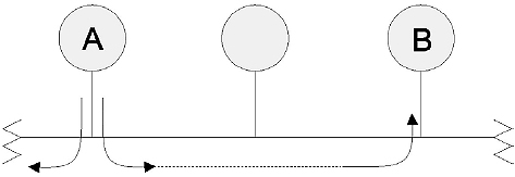
A logical topology defines how the elements in the network communicate with each other and how information is transmitted through a network. The different types of media access methods determine how a node gets to transmit information along the network. In a bus topology information is broadcast, and every node gets the same information within the amount of time it actually takes a signal to propagate down the entire length of cable. This time interval limits the maximum speed and size for the network. In a ring topology each node hears from exactly one node and talks to exactly one other node. Information is passed sequentially, in a predefined order. A polling or token mechanism is used to determine who has transmission rights, and a node can transmit only when it has this right.
A physical topology defines the wiring layout for a network. This specifies how the elements in the network are connected to each other electrically. This arrangement will determine what happens if a node on the network fails. Physical topologies fall into three main categories viz. bus, star, and ring. Combinations of these can be used to form hybrid topologies in order to overcome weaknesses or restrictions in one or other of these three component topologies.
2.8.3 Bus topology
A bus refers to both a physical and a logical topology. As a physical topology a bus describes a network in which each node is connected to a common single communication channel or ‘bus’. This bus is sometimes called a backbone, as it provides the spine for the network. Every node can hear each message packet as it goes past.
Logically, a passive bus is distinguished by the fact that packets are broadcast and every node gets the message at the same time. Transmitted packets travel in both directions along the bus, and need not go through the individual nodes, as in a point-to-point system. Instead, each node checks the destination address included in the frame header to determine whether that packet is intended for it or not. When the signal reaches the end of the bus, an electrical terminator absorbs the packet energy to keep it from reflecting back again along the bus cable, possibly interfering with other frames on the bus. Both ends of the bus must be terminated, so that signals are removed from the bus when they reach the end.
If the bus is too long, it may be necessary to boost the signal strength using some form of amplification, or repeater. The maximum length of the bus is primarily limited by signal attenuation issues. Figure 2.14 illustrates the bus topology.
Bus topology
Advantages of a bus topology
Bus topologies offer the following advantages:
- A bus uses relatively little cable compared to other topologies, and arguably has the simplest wiring arrangement
- Since nodes are connected by high impedance taps across a backbone cable, it is easy to add or remove nodes from a bus. This makes it easy to extend a bus topology
- Architectures based on this topology are simple and flexible
- The broadcasting of messages is advantageous for one-to-many data transmissions
Disadvantages of a bus topology
These include:
- There can be a security problem, since every node may see every message, even those that are not destined for it
- Troubleshooting can be difficult, since the fault can be anywhere along the bus
- There is no automatic acknowledgment of messages, since messages get absorbed at the end of the bus and do not return to the sender
- The bus can be a bottleneck when network traffic gets heavy. This is because nodes can spend much of their time trying to access the network
- In baseband systems a bus can only support half-duplex
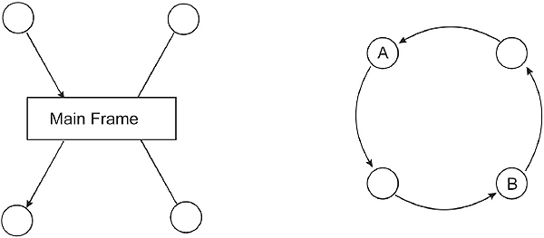
2.8.4 Star topology
In a physical star topology multiple nodes are connected to a central component, generally known as a hub. The hub of a star is often just a wiring center; i.e. a common termination point for the node cables. In some cases the hub may actually be a file server (a central computer that contains a centralized file and control system), with all the nodes attached to it with point-to-point links. When used as a wiring center a hub may, in turn, be connected to the file server or to another hub.
All frames going to and from each node must pass through the hub to which the node is connected. The telephone system is the best known example of a star topology, with lines to individual subscribers coming from a central telephone exchange location.
There are not many LAN implementations that use a logical star topology. The low impedance ARCNet networks are probably the best example. However, the physical layout of many other LANs physically resemble a star topology even though they are logically interconnected in a different way. An example of a star topology is shown in Figure 2.15.

Star topology
Advantages of a star topology
- Troubleshooting and fault isolation is easy
- It is easy to add or remove nodes, and to modify the cable layout
- Failure of a single node does not isolate any other node
- The inclusion of a central hub allows easier monitoring of traffic for management purposes
Disadvantages of a star topology
- If the hub fails, the entire network fails. Sometimes a backup central machine is included, to make it possible to deal with such a failure
- A star topology requires a lot of cable
2.8.5 Ring topology
In a physical ring topology the frames are transmitted sequentially from node to node, in a predefined order. Nodes are arranged in a closed loop, so that the initiating node is the last one to receive a frame. As such it is an example of a point-to-point system.
Information traverses a one-way path, so that a node receives frames from exactly one node and transmits them to exactly one other node. A message frame travels around the ring until it returns to the node that originally sent it. Each node checks whether the message frame’s destination node matches its address. When the frame reaches its destination, the destination node accepts the message and then sends it back to the sender in order to acknowledge receipt.
Since ring topologies use token passing to control access to the network, the token is returned to sender together with the acknowledgment. The sender then releases the token to the next node on the network. If this node has nothing to say, it passes the token on to the next node, and so on. When the token reaches a node with a frame to send, that node sends its frame. Physical ring networks are rare, because this topology has considerable disadvantages compared to a more practical star-wired ring hybrid, which is described later.

Ring topology
Advantages of a ring topology
- A physical ring topology has minimal cable requirements
- No wiring center or closet is needed
- The message can be automatically acknowledged
- Each node can regenerate the signal
Disadvantages of a ring topology
- If any node goes down, the entire ring goes down
- Diagnosis/troubleshooting (fault isolation) is difficult because communication is only one-way
- Adding or removing nodes disrupts the network
As well as these three main topologies, some of the more important variations will now be considered. These are just variations, and should not be considered as topologies in their own right.
2.8.6 Other topologies
Star-wired ring topology
IBM Token Ring networks are the best-known example of a star-wired ring topology. A star-wired ring topology is a hybrid physical topology that combines features of the star and ring topologies. Individual nodes are connected to a central hub, as in a star network. Within the hub, however, the connections are arranged into an internal ring. Thus, the hub constitutes the ring, which must remain intact for the network to function. The hubs, known as Multistation Access Units (MAUs), may be connected to other hubs. In this arrangement, each internal ring is opened and connected to the attached hubs, to create a larger, multi-hub ring.
The advantage of using star wiring instead of simple ring wiring is that it is easy to disconnect a faulty node from the internal ring. The IBM data connector is specially designed to close a circuit if an attached node is disconnected physically or electrically. By closing the circuit, the ring remains intact, but with one less node. In Token Ring networks a secondary ring path can be established and used if part of the primary path goes down. The star-wired ring is illustrated in Figure 2.17.
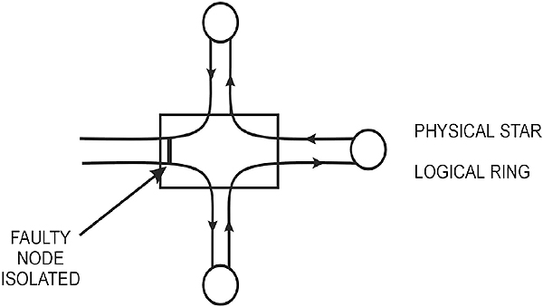
Star-wired ring
The advantages of a star-wired ring topology include:
- Troubleshooting, or fault isolation, is relatively easy
- The modular design makes it easy to expand the network, and makes layouts extremely flexible
- Individual hubs can be connected to form larger rings
- Wiring to the hub is flexible
The disadvantages of a star-wired ring topology include:
- Configuration and cabling may be complicated because of the extreme flexibility of the arrangement.
Distributed star topology
A distributed star topology is a physical topology that consists of two or more hubs, each of which is the center of a star arrangement. A good example of such a topology is an ARCNet network with at least one active hub and one or more active or passive hubs. The 100VG ANYLAN uses a similar topology.

Distributed star topology
Mesh topology
A mesh topology is a physical topology in which there are at least two paths to and from every node. This type of topology is advantageous in hostile environments in which connections are easily broken. If a connection is broken, at least one substitute path is always available. A more restrictive definition requires each node to be connected directly to every other node. Because of the severe connection requirements, such restrictive mesh topologies are feasible only for small networks.

Mesh network
Tree topology
A tree topology, also known as a distributed bus or a branching tree topology, is a hybrid physical topology that combines features of star and bus topologies. Several buses may be daisy-chained together, and there may be branching at the connections (which will be hubs). The starting end of the tree is known as the root or head end. This type of topology is used in delivering cable television services.
The advantages of a tree topology are:
- The network is easy to extend by just adding another branch
- Fault isolation is relatively easy
The disadvantages include:
- If the root goes down, the entire network goes down
- If any hub goes down, all branches off that hub go down
- Access becomes a problem if the entire network becomes too big

Tree topology
2.9 Media access control methods
A common and important method of differentiating between different LAN types is to consider their media access methods. Since there must be some method of determining which node can send a message, this is a critical area that determines the efficiency of the LAN. There are a number of methods that can be considered, of which the two most common in current LANs are the ‘contention’ and ‘token passing’ methods. .
2.9.1 Contention
Contention is the basis for a first-come-first-served media accesses control method. This operates in a similar manner to polite human communication. We listen before we speak, deferring to anyone who already is speaking. If two of us start to speak at the same time, we recognize that fact and both stop, before starting our messages again a little later. In a contention-based access method, the first node to seek access when the network is idle will be able to transmit. Contention is at the heart of the Carrier Sense Multiple Access/Collision Detection (CSMA/CD) access method used by Ethernet.
The ‘carrier sense’ component requires a node to listen out for a ‘carrier’ before it transmits. There is no actual carrier present but the name relates back to the original Aloha project of the University of Hawaii. ’Carrier sense’ in the Ethernet context simply means to listen out for any current transmission on the medium. The length of the channel and the finite signal propagation delay means that there is still a distinct probability that more than one transmitter will attempt to transmit at the same time, as they both will have heard ‘no carrier’. The collision detection logic ensures that more than one simultaneous transmission on the channel will be detected. The system is a probabilistic system, since the exact timing of access to the channel cannot be ascertained in advance.
2.9.2 Token passing
Token passing is a ‘deterministic’ media access method in which a token is passed from node to node, according to a predefined sequence. A token is a special frame consisting of a few bytes that cannot be mistaken for a message. At any given time the token can be available or in use. When an available token reaches a node, that node can access the network for a maximum predetermined time, before passing the token on.
This deterministic access method guarantees that every node will get access to the network within a given length of time, usually in the order of a few milliseconds. This is in contrast to a probabilistic access method (such as CSMA/CD), in which nodes check for network activity when they want to access the network, and the first node to claim the idle network gets access to it. Because each node gets its turn within a fixed period, deterministic access methods are more efficient on networks that have heavy traffic. With such networks, nodes using probabilistic access methods spend much of their time competing to gain access and relatively little time actually transmitting data over the network. Network architectures that support the token passing access method include ARCNet, FDDI, and Token Ring.
To transmit, the node first marks the token as ‘in use’, and then transmits a data packet, with the token attached. In a ring topology network, the packet is passed from node to node, until the packet reaches its destination. The recipient acknowledges the packet by sending the message back to the sender, who then sends the token on to the next node in the network.
In a bus topology network, the next recipient of a token is not necessarily the node that is nearest to the current token passing node. Instead, the next node is determined by some predefined rule. The actual message is broadcast on to the bus for all nodes to ‘hear’. For example, in a Modbus Plus network the token is passed on to the node with the next higher network address. Networks that use token passing generally have some provision for setting the priority with which a node gets the token. Higher-level protocols can specify that a message is important and should receive higher priority.

Token passing
A Token Ring network requires an Active Monitor (AM) and one or more Standby Monitors (SMs). The AM keeps track of the token to make sure it has not been corrupted, lost, or sent to a node that has been disconnected from the network. If any of these things happens, the AM generates a new token, and the network is back in business. The SM makes sure the AM is doing its job and does not break down and get disconnected from the network. If the AM is lost, one of the SMs becomes the new AM, and the network resumes operation. These monitoring capabilities result in complex circuitry on the NICs.
The deterministic nature of token passing does not necessarily mean fast access to the bus, but merely predictable access to the bus. A heavily loaded Modbus Plus network can have a token rotation time of 500 milliseconds!
2.9.3 Polling
Polling refers to a process of checking elements such as computers or queues, in some defined order, to see whether the polled element needs attention (wants to transmit, contains jobs, and so on). In roll call polling, the polling sequence is based on a list of elements available to the controller. In contrast, in hub polling, each element simply polls the next element in the sequence.
In LANs, polling provides a deterministic media access method in which the controller polls each node in succession to determine whether that node wants to access the network. In some systems the polling is done by means of software messages being passed to and fro, which could slow down the process. In order to overcome this problem, systems such as 100VG AnyLAN employ a hardware-polling mechanism that uses voltage levels to determine whether a node needs to be serviced or not.
Learning objectives
When you have completed study of this chapter you should be able to:
- Describe the major hardware components of an IEEE 802.3 CSMA/CD network
- Explain the method of connection for 10Base2, 10Base5 and 10BaseT networks
- Explain the operation of CSMA/CD
- Describe the fields in the IEEE 802.3 (Ethernet) data frame
- Describe the causes of Ethernet collisions and how to reduce them
3.1 The origins of Ethernet
The Ethernet network concept was developed by Xerox at its Palo Alto Research Center (PARC) in the mid-seventies. It was based on the work done by researchers at the University of Hawaii where campus sites on the various islands were interconnected with the ALOHA network, using radio as the medium. This network was colloquially known as ‘Ethernet’ since it used the ‘ether’ as the transmission medium.
The philosophy was quite straightforward. Any station that wanted to broadcast to another station would do so without deferring to any transmission in progress. The receiving station then had the responsibility of acknowledging the message, advising the transmitting station of a successful reception. This primitive system did not rely on any detection of collisions (two radio stations transmitting at the same time) but, instead, expected acknowledgment within a predefined time.
The initial system was so successful that Xerox soon applied it to their other sites, typically interconnecting office equipment and shared resources such as printers and computers acting as repositories of large databases.
In 1980 the Ethernet Consortium consisting of Xerox, Digital Equipment Corporation and Intel (the DIX consortium) issued a joint specification based on the Ethernet concept, known as Ethernet Version 1. This was later superseded by the Ethernet Version 2 (Blue Book) specification. Version 2 was offered to the IEEE for ratification as a formal standard and in 1983 the IEEE issued the IEEE 802.3 CSMA/CD (Ethernet) standard.
Although IEEE 802.3 effectively replaced the old standard, the Blue Book legacy still remains in the form of a slightly different data encapsulation in the frame. This is, however, a software issue.
Later versions of Ethernet (from 100 Mbps upwards) also support full-duplex, although they have to support CSMA/CD for the sake of backward compatibility. Industrial versions of Ethernet typically operate at 100 Mbps and above in full-duplex mode, and often support the IEEE 802.1p/Q modified (tagged) frame structure. This allows a reasonable degree of deterministic operation. Many modern Ethernet based field buses make use of additional measures such as the IEEE 1588 clock synchronizing standard to achieve real-time operation with deterministic behavior in the microsecond region.
3.2 Physical layer implementations
The original IEEE 802.3 standard defines a range of cable types. They include coaxial, twisted pair and fiber optic cable. Despite 10 Mbps Ethernet being a legacy technology, it is still used in older installations and therefore a brief overview of the technology is in order. In addition, many of the design issues in the newer versions can only be understood against the backdrop of the original technology.
The IEEE 802.3 standard has several variants. Many of them died an early death, but the following versions are still used in older installations:
-
- 10Base5
Thick wire coaxial cable (RG-8), single cable bus
-
- 10Base2
Thin wire coaxial cable (RG-8), single cable bus
-
- 10BaseT
Unscreened Twisted Pair cable (TIA/IEA 568B Cat3) star topology
-
- 10BaseFL
Optical fiber, 10 Mbps, twin fiber point to point
3.2.1 10Base5
10Base5 (Thicknet) is a legacy technology but some systems are still in use in industrial applications. We will therefore deal with it rather briefly. It uses a coaxial cable as a bus (also referred to as a ‘trunk’). The RG-8 cable has a 50-ohm characteristic impedance and is yellow or orange in color. The naming convention ‘10Base5’ indicates a 10 Mbps data rate, baseband signaling, and 500-meter segment lengths. The cable is difficult to work with, and so cannot normally be taken to the node directly. Instead, it is laid in a cabling tray and the transceiver electronics (the Medium Attachment Unit or MAU) is installed directly on the cable. From there an intermediate cable, known as an Attachment Unit Interface (AUI) cable is used to connect to the NIC. The AUI cable can be up to 50 meters long. and consists of 5 individually shielded pairs viz. two pairs each for transmit and receive (control plus data) plus one for power.
The MAU connection to the trunk is made by cutting the cable and inserting an N-connector and a coaxial T-piece, or by using a ‘vampire’ tap. The latter is a mechanical connection that clamps directly over the cable. Electrical connection is made via a screw-in probe that connects to the center conductor, and sharp teeth that puncture the cable sheath to connect to the braid. These hardware components are shown in Figure 3.1.

10Base5 hardware components
The location of the connection is important to avoid multiple electrical reflections on the cable and the trunk cable is marked every 2.5 meters with a black or brown ring to indicate where a tap should be placed. Fan-out boxes can be used if there are a number of nodes to be connected, allowing a single tap to feed multiple nodes. Connection at either end of the AUI cable is made through a 25-pin D-connector, with a slide latch, often called a DIX connector. This has been shown in Figure 3.2.

AUI cable
There are certain rules to be followed. These include:
- Segments must be less than 500 meters in length
- There may be no more than 100 taps on each segment
- Taps must be placed at integer multiples of 2.5 meters
- The cable must be terminated with a 50-ohm terminator at each end
- One end of the cable shield must be grounded
The physical layout of a 10Base5 segment is shown in Figure 3.3

10Base5 Ethernet segment
With 10Base5 there is no on-board transceiver on the NIC. Instead, the transceiver is located in the MAU and this is fed with power from the NIC via the AUI cable. Since the transceiver is now remote from the NIC, the node needs to be aware that the termination can detect collisions if they do occur. This confirmation is performed by a Signal Quality Error (SQE), or heartbeat, test function in the MAU. The SQE signal is sent from the MAU to the node on detecting a collision on the bus. However, on completion of every frame transmission by the MAU, the SQE signal is also sent to ensure that the circuitry remains active, and that collisions can be detected. Mixing devices that support SQE with those that don’t could cause problems, as non-SQE-enabled NICs could perceive ‘normal’ SQE pulses as collisions, leading to jam signals and repetitive re-broadcasting of messages.
3.2.2 10Base2
The other type of coaxial cable Ethernet network is 10Base2 and this is sometimes referred to as ‘Thinnet’ or ‘thinwire Ethernet’. It uses the thinner (5 mm diameter) RG-58 A/U or C/U coax cable with a 50-ohm characteristic impedance. The cable is connected to the 10Base2 NICs or 10Base5 MAUs by means of BNC T-piece connectors.
Connectivity requirements stipulate that:
- It must be terminated at each end with a 50-ohm terminator
- The maximum length of a cable segment is 185 meters
- No more than 30 transceivers may be connected to any one segment
- There must be a minimum spacing of 0.5 meters between nodes
- It may not be used as a link segment between two ‘Thicknet’ segments
- The minimum bend radius is 5 cm
The physical layout of a 10Base2 Ethernet segment is shown in Figure 3.4.

10Base2 Ethernet segment
3.2.3 10BaseT
10BaseT uses Cat3 (or better) AWG24 UTP cable for connection to the node. The physical topology is a star, with nodes connected to hub. Logically it forms a (chained) bus, since when one station transmits all others can ‘hear’ it. The four-pair cable from hub to node has a maximum length of 100 meters. One pair is used for receive and another is used for transmit. The connectors specified are RJ-45. Figure 3.5 shows schematically how the 10BaseT nodes are interconnected by the hub. This is also known as a ‘chained bus’ configuration, as opposed to 10Base5 and 10Base2 that are ‘branched bus’ configurations.

Schematic 10BaseT system
Collisions are detected by the NIC and so a signal received by the hub must be retransmitted on all ports. The electronics in the hub must also ensure that the stronger retransmitted signal does not interfere with the weaker input signal. The effect is known as far end crosstalk (FEXT), and is handled by special adaptive crosstalk echo cancellation circuits.
The 10BaseT star topology became very popular but has been largely superseded by faster versions such as Fast and Gigabit Ethernet. The shared hubs have also been replaced with switching hubs, and the preferred mode of operation is full-duplex instead of CSMA/CD. This will be discussed in the next chapter.
3.2.4 10BaseF
The 10BaseF was a star topology using wiring hubs, and comprised three variants namely 10BaseFL, 10BaseFP and 10BaseFB. Of these, only 10BaseFL survived. 10BaseFL is a point-to-point technology using two fibers, with a range of 2000m.
3.3 Signaling methods
10 Mbps Ethernet signals are encoded using Manchester encoding as described in chapter 1, which allows the clock to be extracted at the receiver end in order to synchronize the transmission/reception process
The voltage swings were from –0.225 to –1.825 volts in the original Bluebook Ethernet specification. In IEEE 802.3 voltages on coax cables are specified to swing between 0 and –2.05 volts with a rise and fall time of 25 ns at 10 Mbps. IEEE 802.3 voltages on UTP swing between -0.7V and +0.7V .
3.4 Medium access control
The method used is one of contention. Each node has a connection via a transceiver to the common bus. The transceiver can transmit and receive simultaneously. It can, therefore, be in any one of three states namely idle (listen only), transmit, or be in contention. In the idle state the node merely listens to the bus, monitoring all traffic. If it then wishes to transmit information, it will defer whilst there is any activity on the bus since this is the ‘carrier sense’ component of the access method. At some stage the bus will become silent. After a period of 96 bit times, known as the inter-frame gap (to allow the passing frame to be received and processed by the destination node) the transmission process commences. The node is now in the transmit mode, and will transmit and listen at the same time. This is because there is no guarantee that another node at some other point on the bus has not also started transmitting having recognized the absence of traffic.
After a short delay, as the two signals propagate towards each other on the cable, there will be a collision of signals. Obviously the two transmissions cannot coexist on the common bus, since this is a baseband system. The transceiver detects this collision, since it is monitoring both its input and output, and recognizes the difference. The node now goes into a state of contention. It will continue to transmit for a short time (the jam signal) to ensure the other transmitting node detects the contention, and then perform a back-off algorithm to determine when it should again attempt to transmit its waiting frames.
3.5 Frame transmission
Since there is a finite time for the transmission to propagate to the ends of the bus, and thus ensure that all nodes recognize that the medium is busy, the transceiver turns on a collision detection circuit whilst the transmission takes place. Once a certain number of bits (576) have been transmitted, provided that the network cable segment specifications have been complied with, the collision detection circuitry can be disabled. If a collision should take place after this, it will be the responsibility of higher level protocols to request retransmission. This is a far slower process than the hardware collision detection process.
Here is a good reason to comply with cable segment specifications. The initial ‘danger’ period is known as the collision window and is effectively twice the time interval for the first bit of a transmission to propagate to all parts of the network. The ‘slot time’ for the network is then defined as the worst-case time delay that a node must wait before it can reliably know that a collision has occurred. This is defined as:
Slot time = 2 * (transmission path delay) + safety margin
The slot time is fixed at 512 bits or 64 bytes, i.e. 51.2 microseconds for 10 Mbps Ethernet.
3.6 Frame reception
The transceiver of each node is constantly monitoring the bus for a signal. As soon as one is recognized, the NIC activates a carrier sense signal to indicate that transmissions cannot be made. The first bits of the MAC frame are a preamble and consist of 56 bits of 1010 etc. On recognizing these, the receiver synchronizes its clock and converts the Manchester encoded signal back into binary form. The eighth byte is a start of frame delimiter, and is used to indicate to the receiver that it should strip off the first eight bytes and commence determining whether this frame is for its node by reading the destination address in the frame header. If the address is recognized, the data is loaded into a frame buffer within the NIC.
Further processing then takes place, including the calculation and comparison of the frame CRC, and checking it against with the transmitted CRC. The NIC also checks that the frame contains an integral number of bytes and is neither too short nor too long. Provided all is correct, the frame is passed to the Data Link layer for further processing.
3.7 Collisions
Collisions are a normal part of a CSMA/CD network since the monitoring and detection of collisions is the method by which a node ensures unique access to the shared medium. It is only a problem when there are excessive collisions. This reduces the available bandwidth of the cable and slows the system down while retransmission attempts occur. There are many reasons for excessive collisions and this will be addressed shortly.
The principle of collision cause and detection is shown in the following diagram.

CSMA/CD collisions
Assume that both node 1 and node 2 are in listen mode and node 1 has frames queued to transmit. All previous traffic on the medium has ceased, and the inter-frame gap from the last transmission has expired. Node 1 now commences to transmit its preamble signal, which propagates both left and right across the cable. At the left end the termination resistance absorbs the transmission, but the signal continues to propagate to the right. However, the Data Link layer in node 2 also has a frame to transmit and since the NIC ‘sees’ a free cable, it also commences to transmit its preamble. Again, the signals propagate down the cable, and some short time later they ‘collide’. Almost immediately, node 2’s transceiver recognizes that the signals on the cable are corrupted, and the logic incorporated in the NIC asserts a collision detect signal. This causes node 2 to send a jam signal of 32 bits, and then stop transmitting. The standard allows any data to be sent as long as, by design, it is not the value of the CRC field of the frame. It appears that most nodes will send the next 32 bits of the data frame as a jam, since that is instantly available.
This jam signal continues to propagate along the cable, superimposed on the signal still being transmitted from node 1. Eventually node 1 recognizes the collision, and goes through the same jam process as node 2. The frame from node 1 must therefore be at least twice the end-to-end propagation delay of the network, or else the collision detection will not work correctly. The jam signal from node 1 will continue to propagate across the network until absorbed at the far end terminator, meaning that the system vulnerable period is three times the end to end propagation delay.
After the jam sequence has been sent, the transmission is halted. The node then schedules a retransmission attempt after a random delay controlled by a process known as the truncated binary exponential back off algorithm. The length of the delay is chosen so that it is a compromise between reducing the probability of another collision and delaying the retransmission for an unacceptable length of time. The delay is always an integer multiple of the slot time. In the first attempt the node will choose, at random, either one or zero slot times delay. If another collision occurs, the delay will be chosen at random from 0, 1, 2 or 3 slot times, thus reducing the probability that a further collision will occur. This process can continue for up to 10 attempts, with a doubling of the range of slot times available for the node to delay transmission at each attempt. After ten attempts the node will attempt 6 more retries, but the slot times available for the delay period will remain as they were at the tenth attempt. After sixteen attempts it is likely that there is a problem on the network and the node will cease to retransmit.
3.8 Frame format
The basic Ethernet/IEEE 802.3 frame format is shown below. Each field in the frame will now be described in detail.

Frame format
3.8.1 Synchronization
This field is used for the synchronization of the receiver clocks.
3.8.2 Preamble
This consists of 7 bytes containing 10101010, resulting in a square wave being transmitted. The preamble is used by the receiver to synchronize its clock to the transmitter.
3.8.3 Start Frame Delimiter (SFD)
This single byte field consists of 10101011. It enables the receiver to recognize the commencement of the address fields. Technically speaking this is just another byte of the preamble and, in fact, in the Ethernet version 2 specification it was simply viewed as part of an 8-byte preamble.
3.8.4 Header
This field contains three fields, allocated as follows:
3.8.5 Source and Destination Address
These are the physical addresses of both the source and destination nodes and are usually embedded in the firmware of the NICs. The fields are 6 bytes long and made up of two three-byte blocks. The first three bytes are known as the Organizationally Unique Identifier (OUI) and identifies the manufacturer. This is administered by the IEEE. The second block is the device identifier, and each card will have a unique address under the terms of the license to manufacture. This means there are 224 unique addresses for each OUI. These addresses are known as MAC addresses, media addresses or hardware addresses.
There are three addressing modes:
-
- Broadcast
The destination address is set to all ‘1’s or FF-FF-FF-FF-FF-FF
-
- Multicast
The first bit of the destination address is set to a 1. It provides group restricted communications
-
- Individual, or point-to-point
First bit of the address is 0. A typical unicast MAC address is 00-06-5B-12-45-FC
3.8.6 Length/Type
This two-byte field contains the length of the data field. If the frame is transmitted in Blue Book format, then this field contains an IEEE registered ‘type’ number, identifying the higher level protocol that is sending the data. An example is 0x800 (800 Hex) for IP. It is easy for the software to take care of this, since any number larger than 1500 (maximum number of data bytes) denotes a type number.
3.8.7 Data
The information that has been handed down to the Data Link layer for transmission. This varies from 0 to 1500 bytes.
The padding is conceptually part of the data field. Since the minimum frame length is 64 bytes (512 bits), the pad field will pad out any frame that does not meet this minimum specification. This pad, if incorporated, is normally random data. The CRC is calculated over the data in the pad field. Once the CRC checks OK, the receiving node discards the pad data. Pad data therefore varies between 0 and 46 bytes.
3.8.8 Frame Check Sequence
A 32-bit CRC value that is computed in hardware at the transmitter and appended to the frame. It is the same algorithm used in the IEEE 802.5 standard.
3.9 Reducing collisions
The main reasons for collision rates on a half-duplex Ethernet network are:
- The number of packets per second
- The signal propagation delay between transmitting nodes
- The number of stations initiating packets
- The bandwidth utilization
A few suggestions on reducing collisions are:
- Keep all cables as short as possible
- Keep all high activity sources and their destinations as close as possible. Possibly isolate these nodes from the main network backbone with bridges/routers to reduce backbone traffic
- Use buffered repeaters rather than bit repeaters
- Check for unnecessary broadcast packets that are aimed at non-existent nodes
- Remember that the monitoring equipment to check out network traffic can contribute to the traffic (and the collision rate)
3.10 Half-duplex Ethernet design rules
Legacy (half duplex) Ethernet systems had several ‘design rules’, that are irrelevant in the context of modern high-performance switched full duplex systems. However, an awareness of these rules may be necessary in the case of maintenance work, so they are briefly addressed here.
It is important to maintain the overall Ethernet requirements as far as length of the cable is concerned. Each variant (e.g. 10Base5) has a particular maximum segment length allowable. The recommended maximum length is 80% of this figure.
Coaxial cable segments need not be made from a single homogenous length of cable, and may comprise multiple lengths joined by coaxial connectors. Although 10Base5 and 10Base2 cables have the same nominal 50-ohm impedance they can only be mixed within the same 10Base2 cable segment (not within a 10Base5 segment) to achieve greater segment length.
On 10Base5 cable segments it is preferable that the total segment be made from one length of cable or from sections off the same drum of cable. If multiple sections of cable from different manufacturers are used, then these should be standard lengths of 23.4 m, 70.2 m or 117 m (± 0.5 m), which are odd multiples of 23.4 m (half wavelength in the cable at 5 MHz). These lengths ensure that reflections from the cable-to-cable impedance discontinuities are unlikely to add in phase. Using these lengths exclusively a mix of cable sections should be able to be made up to the full 500 m segment length.
If the cable is from different manufacturers and there are potential mismatch problems, it should be confirmed that signal reflections due to impedance mismatches do not exceed 7% of the incident wave.
In 10Base5 systems the maximum length of the transceiver cables is 50 m but this only applies to specified IEEE 802.3 compliant cables. Other AUI cables using ribbon or office grade cables can only be used for short distances (less than 12.5 m).
Connection of MAUs to the cable causes signal reflections due to their bridging impedance. Their placement must therefore be controlled to ensure that these reflections do not significantly add in phase. In 10Base5 systems the MAUs are spaced at 2.5 m multiples, coinciding with the cable markings. In 10Base2 systems the minimum MAU spacing is 0.5 m.
The maximum bus length is made up of five segments, connected by four repeaters. The total number of segments can be made up of a maximum of three coax segments, containing nodes, and two 10BaseFL link segments (see Figure 3.8). This is referred to as the ‘5-4-3-2 rule’ and the number of repeaters is referred to as the ‘repeater count’. It is important to verify that the above transmission rules are met by all paths between any two nodes on the network.

Maximum transmission path
The maximum network size is, therefore, as follows:
- 10Base5 = 2800 m node to node
(5 × 500 m segments + 4 repeater cables + 2 AUI) - 10Base2 = 925 m node to node (5 × 185 m segments)
- 10BaseT = 100 m node to hub
IEEE 802.3 states that the shield conductor of the RG-8 coaxial cable should make electrical contact with an effective ground reference at one point only. This is normally done at a terminator, since most RG-8 terminators have a screw terminal to which a ground lug can be attached, preferably using a braided cable, to ensure good grounding.
All other splices, taps or terminators should be jacketed so that no contact can be made with any metal objects. Insulating boots or sleeves should be used on all in-line coaxial connectors to avoid unintentional ground contact.
Learning objectives
When you have studied this chapter you should be able to:
- List the basic methods used to achieve high transmission speeds on UTP cable
- Describe the operation of 100Base-T
- List the different physical media options for 100Base-T systems
- Explain the basic differences between Class I and Class II hubs (‘repeaters’)
- Explain the packet bursting technique used by Gigabit Ethernet
- Describe the different media options used by Gigabit Ethernet
4.1 Achieving higher speed
Although 10 Mbps Ethernet with over 200 million installed nodes world-wide became the most popular method of linking computers on networks, its speed was too slow for data- intensive or real-time applications.
From a philosophical point of view there are several ways to increase speed on a network. The easiest, conceptually, is to increase the bandwidth and allow faster changes of the data signal. This requires a high bandwidth medium and generates a considerable amount of high frequency electrical noise on copper cables, which is difficult to suppress. The second approach is to move away from the serial transmission of data on one circuit to a parallel transmission over multiple circuits. A third approach is to use data compression techniques in order to transfer multiple bits for each electrical transition. A fourth approach (used with Gigabit Ethernet) is to operate circuits in full-duplex mode, allowing simultaneous transmission in both directions. All these approaches are used to implement 100 Mbps Fast Ethernet and 1000 Mbps Gigabit Ethernet transmission on fiber optic as well as copper cables.
Typically most LAN systems use coaxial cable, Shielded Twisted Pair (STP), Unshielded Twisted Pair (UTP) or fiber optic cables. The capacitance of the coaxial cable imposes a serious limit on the distance over which the higher frequencies can be handled and also prohibits the use of full duplex. Consequently 100 Mbps systems do not use coaxial cable.
The UTP is obviously popular because of ease of installation and low cost. This is the basis of the 10BaseT Ethernet standard. The Cat3 cable allows only 10 Mbps over 100m while Cat5 allows 100 Mbps data rates over 100m. The four pairs in the standard cable allow several parallel data streams to be handled.
Fiber optic cables have enormous bandwidths and excellent noise immunity, thus they are the obvious choice for long-haul connections and installation in areas with a high degree of noise.
4.2 100Base-T
The 100Base-T variants use the existing Ethernet MAC layer with various enhanced Physical Media Dependent (PMD) sub-layers to improve the speed. They are described in the IEEE 802.3u and 802.3y standards as follows.
IEEE 802.3u defines three variants, namely:
- 100Base-TX, which uses two pairs of Cat5 UTP or STP
- 100Base-T4, which uses four pairs of wires of Cat3, 4 or 5 UTP
- 100Base-FX, which uses multi-mode or single-mode fiber optic cable
100Base-TX and 100Base-FX are collectively known as 100Base-X. Another specification, IEEE 802.3y, defines a single variant, 100Base-T2, which uses two pairs of wires of Cat3 or better. 100Base-T2 was, unfortunately, released much later than its counterparts and did not ‘make it’ to the marketplace, with the result that most documents and articles on Fast Ethernet do not even refer to it. 100Base-BX and 100Base-LX10 are the new versions of Fast Ethernet.
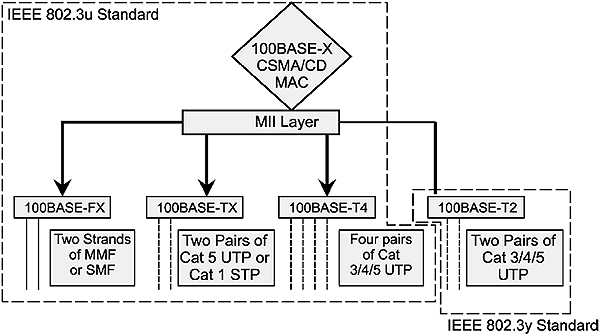
Summary of 100Base-T standards
The approach illustrated in Figure 4.1 is possible because the original IEEE 802.3 specifications defined the MAC sub-layer independently of the various physical PMD layers it supports. The MAC sub-layer defines the format of the Ethernet frame as well as the operation of the CSMA/CD mechanism. The time dependent parameters are defined in IEEE 802.3 in terms of bit-time intervals, so they are speed dependent. The 10 Mbps Ethernet inter-frame gap is actually defined as a time interval of 96 bit times, which translates to 9.6 microseconds for 10 Mbps Ethernet and 960 nanoseconds for Fast Ethernet.
One of the limitations of 100Base-T systems operating in half-duplex mode is the size of the collision domain, which is 250 m. This is the maximum size network in which collisions can be detected; ten times smaller than the maximum size of a 10 Mbps network. Since the distance between workstation and hub is limited to 100 m, the same as with 10BaseT, and usually only one hub is allowed in a collision domain, networks larger than 200 m must be logically interconnected by store-and-forward type devices such as bridges, routers or switches. This is not necessarily a bad thing, since it segregates the traffic within each collision domain, reducing the number of collisions on the network.
Since all modern Fast Ethernet systems (especially industrial implementations) are full duplex in any case, this is not really a problem.
The dominant 100Base-T systems are 100Base-TX and 100Base-FX. The other two variants are only included here from an academic viewpoint.
100Base-BX was developed to provide service over a single strand of optical fiber (unlike 100Base-FX, which uses a pair of fibers). Single-mode fiber along with a special multiplexer splits the signal into transmit and receive wavelengths (1310/1550nm). The terminals on each side of the fiber are not equal, as downstream transmission uses a wavelength of 1550nm, and upstream transmission uses 1310 nm wavelength. It has a nominal reach of 10, 20 or 40 km.
The version 100Base-LX10 provides service over two single-mode optical fibers up to 10 km using 1310 nm wavelength.
4.2.1 IEEE 802.3u 100Base-T standards arrangement
The IEEE 802.3u standard fits into the OSI model as shown in Figure 4.2. Note that the unchanged IEEE 802.3 MAC layer sits beneath the LLC sub-layer as the lower half of the Data Link layer of the OSI model.
Its Physical layer is divided into the following sub-layers and their associated interfaces:
- PHY – Physical medium independent layer
- MII – Medium Independent Interface
- PMD – Physical Medium Dependent layer
- MDI – Medium Dependent Interface
A convergence sub-layer is added for the 100Base-TX and FX systems, which use the ANSI X3T9.5 PMD layer developed for the twisted pair version of FDDI. The FDDI PMD layer operates as a continuous full-duplex 125 Mbps transmission system, so a convergence layer is needed to translate this into the 100 Mbps half-duplex data bursts expected by the IEEE 802.3 MAC layer.

100Base-T standards architecture
4.2.2 PHY and PMD sub-layers
The PHY layer specifies 4B/5B coding of the data, data scrambling and the non return to zero – inverted (NRZI) data coding together with the clocking, data and clock extraction processes. The 4B/5B technique is described in Chapter 1.
The PMD sub-layer uses the ANSI TP-X3T9.5 PMD layer and operates on two pairs of Cat5 cable. It uses stream cipher scrambling for data security and MLT-3 bit encoding as described in Chapter 1. Hence for a 31.25 MHz baseband signal this allows for a 125 Mbps signaling bit stream providing a 100 Mbps throughput (4B/5B encoder). The MAC outputs a NRZ code. This code is then passed to a scrambler, which ensures that there are no invalid groups in its NRZI output. The NRZI converted data is passed to the three level code block and the output is then sent to the transceiver.
The three-level code results in a lower frequency signal. Noise tolerance is not as high as in the case of 10BaseT because of the multi-level coding system, hence Cat5 cable is required.
Cat5 wire, RJ-45 connectors and a hub or switch are requirements for 100Base-TX. These factors and a maximum distance of 100 m between the nodes and hubs result in an architecture identical to that of 10BaseT.
4.2.3 100Base-T hubs and adapters
The IEEE 802.3u specification defines two classes of 100Base-T hubs, also called ‘repeaters’:
- Class I (translational) hubs, which can support both TX/FX and T4 systems
- Class II (transparent) hubs, which support only one signaling system
Class I hubs have a greater delay (0.7 μs maximum) and so only permit one hub in a collision domain. The class I hub fully decodes each incoming TX or T4 packet into its digital form at the MII; then sends the packet out as an analog signal from each of the other ports in the hub. Hubs are available with all T4 ports, all TX ports or combinations of TX and T4 ports. The latter are called translational hubs. Their layout is shown in Figure 4.4.
Class II hubs operate like 10BaseT hubs, connecting the ports (all of the same type) at the analog level. These then have lower inter-repeater delays (0.46 μs maximum) and so two repeaters are permitted in the same collision domain, but only 5 m apart. Alternatively, in an all-fiber network, the total length of all the fiber segments is 228 meters. This allows two 100 m segments to the nodes with 28 m between the hubs or any other combination. Most Fast Ethernet hubs available today are class II.

Class I and class II Fast Ethernet hubs
100Base-T adapter cards (NICs) are readily available as standard 100Mbps and as 10/100Mbps. These cards are interoperable at the hub at both speeds.
4.3 Fast Ethernet design considerations
4.3.1 UTP cabling distances
As in the case of 10BaseT, the maximum distance between hub and NIC is 100 meters, made up as follows:
- 5 meters from hub to patch panel
- 90 meters horizontal cabling from patch panel to office punch-down block
- 5 meters from punch-down block to desktop NIC
4.3.2 Fiber optic cable distances
The following maximum cable distances are in accordance with the 100Base-T bit budget (see next section). These are only applicable to 100Base-FX hubs. With switches there is no distance limitation, and distances between 3km (multimode fiber) and 120 km (single mode fiber) are common.
- Node to hub: the maximum distance of multimode cable (62.5/125) is 160 meters for connections using a single Class II hub.
- Node to switch: the maximum multimode cable distance is 210 meters.
- Switch-to-switch: the maximum distance of multimode cable for a backbone connection between two 100Base-FX switch ports is 412 meters.
- Switch-to-switch, full-duplex: maximum distance of multimode cable for a full-duplex connection between two 100Base-FX switch ports is 2000 meters.
4.3.3 100Base-T hub rules
The cable distance and the number of hubs that can be used in a 100Base-T collision domain depend on the delay in the cable, the time delay in the hubs and NIC delays. The maximum round-trip delay for 100Base-T systems is the time to transmit 64 bytes or 512 bits, and equals 5.12 μs. A frame has to go from the transmitter to the most remote node and back to the transmitter for collision detection within this round trip time. Therefore the one-way time delay will be half this.
The maximum-sized collision domain can then be determined by the following calculation:
Repeater delays + Cable delays + NIC delays + Safety factor (5 bits min.) < 2.56μs
Table 4.1 gives typical maximum one-way delays for various components. Hub and NIC delays for specific components can be obtained from the manufacturers.
Maximum one-way Fast Ethernet component delays
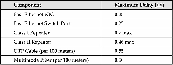
Notes
If the desired distance is too great it is possible to create a new collision domain by using a switch instead of a hub.
Most 100Base-T hubs are stackable, which means that multiple units can be placed on top of each other and interconnected by means of a fast backplane bus. Such connections do not count as repeater hops and make the ensemble function as a single repeater.
4.3.4 Sample calculation
Can two Fast Ethernet nodes be interconnected via two class II hubs that are connected by 50 m fiber? One node is connected to the first hub with 50 m UTP while the other has a 100 m fiber connection to the second hub.
Calculation: Using the time delays in Table 4.2:
Time delays

The total one-way delay of 2.445 μs is within the required interval (2.56 μs) and allows a safety factor of at least 5 bits, so this connection is permissible.
4.4 Gigabit Ethernet
4.4.1 Overview
Gigabit Ethernet uses the same IEEE 802.3 frame format as 10 Mbps and 100 Mbps Ethernet systems. It operates at ten times the clock speed of Fast Ethernet, i.e. at 1Gbps. By retaining the same frame format as the earlier versions of Ethernet, backward compatibility is assured.
Gigabit Ethernet is defined in the IEEE 802.3z and IEEE 802.3ab standards. IEEE 802.3z defines the Gigabit Ethernet Media Access Control (MAC) layer functionality as well as three different physical layers viz. 1000Base-LX and 1000Base-SX using fiber, and 1000Base-CX using copper. These physical layers were originally developed by IBM for the ANSI Fiber channel systems and use 8B/10B encoding to reduce the bandwidth required to send high-speed signals. The IEEE merged the fiber channel with the Ethernet MAC using a Gigabit Media Independent Interface (GMII), which defines an electrical interface, allowing existing fiber channel PHY chips to be used and future physical layers to be easily added. The newer versions of Gigabit Ethernet include 1000BASE-LX10, 1000BASE-BX10, 1000BASE-ZX, and 1000BASE-TX.
1000Base-T was developed to provide service over four pairs of Cat5 or better copper cable. This development is defined by the IEEE 802.3ab standard.
The Gigabit Ethernet versions are summarized in Figure 4.4.

Gigabit Ethernet versions
4.4.2 MAC layer
Gigabit Ethernet retains the standard IEEE 802.3 frame format. However, the CSMA/CD algorithm has had to undergo a small change to enable it to function effectively at 1 Gbps. The slot time of 64 bytes used with both 10 Mbps and 100 Mbps systems had to be increased to 512 bytes. Without this increased slot time the network would have been impractically small at one tenth of the size of Fast Ethernet – only 20 meters! The irony of the matter is that all practical Gigabit Ethernet systems run in full duplex mode and this restriction is therefore irrelevant. However, CSMA/CD compatibility has to be built in for adherence to the IEEE 802.3 standard.
The slot time defines the time during which the transmitting node retains control of the medium, and is an important aspect of the collision detection mechanism. With Gigabit Ethernet it was necessary to increase this time by a factor of eight to 4.096 μs in order to compensate for the tenfold speed increase. This results in a collision domain of about 200m.
If the transmitted frame is less than 512 bytes, the transmitter continues transmitting to fill the 512-byte window. Carrier extension symbols are used to fill the remainder of those frames that are shorter than 512 bytes. This is shown in Figure 4.5.

Carrier extension
While this is a simple technique to overcome the network size problem, it could result in very low network utilization if a lot of short frames are sent, typical of some industrial control systems. For example, a 64-byte frame would have 448 carrier extension symbols attached, and result in a network utilization of less than 10%. This is unavoidable, but its effect can be mitigated by a technique called packet bursting. Once the first frame in a burst has successfully passed through the 512-byte collision window, using carrier extension if necessary, transmission continues with additional frames being added to the burst until the burst limit of 8192 bytes is reached. This process averages the time wasted sending carrier extension symbols over a number of frames.

Packet bursting
4.4.3 PHY sub-layer
The IEEE 802.3z Gigabit Ethernet standard uses the three PHY sub-layers from the ANSI X3T11 fiber channel standard for the 1000Base-SX and 1000Base-LX versions using fiber optic cable and 1000Base-CX using shielded 150-ohm twin-ax copper cable.
The Fiber Channel PMD sub-layer runs at 1 Gbaud and uses the 8B/10B coding of the data, data scrambling and NRZI data coding together with the clocking, data and clock extraction processes. This results in a data rate of 800 Mbps. The IEEE then had to increase the speed of the fiber channel PHY layer to 1250 Mbaud to obtain the required throughput of 1 Gbps.
The 8B/10B technique selectively codes each group of eight bits into a ten-bit symbol. Each symbol is chosen so that there are at least two transitions from ‘1’ to ‘0’ in each symbol. This ensures there will be sufficient signal transitions to allow the decoding device to maintain clock synchronization from the incoming data stream. The coding scheme allows unique symbols to be defined for control purposes, such as denoting the start and end of packets and frames as well as instructions to devices.
The coding also balances the number of ‘1’s and ‘0’s in each symbol, called DC balancing. This is done so that the voltage swings in the data stream will always average to zero, and not develop any residual DC charge, which could result in a distortion of the signal (‘baseline wander’).
4.4.4 1000Base-SX
This Gigabit Ethernet version was developed for the short backbone connections of the horizontal network wiring. The SX systems operate full-duplex with multimode fiber only, using the cheaper 850 nm wavelength laser diodes. The maximum distance supported varies between 200 and 550 meters depending on the bandwidth and attenuation of the fiber optic cable used. The standard 1000Base-SX NICs available today are full-duplex and incorporate SC fiber connectors.
4.4.5 1000Base-LX
This version was developed for use in the longer backbone connections of the vertical network wiring. The LX systems can use single mode or multimode fiber with the more expensive 1300 nm laser diodes. The maximum distance recommended by the IEEE for these systems operating in full-duplex is 5 km for single mode cable and 550 meters for multimode fiber cable. Many 1000Base-LX vendors guarantee their products over a much greater distance; typically 10 km. Fiber extenders are available to allow service over as much as 80 km. The standard 1000Base-LX NICs available today are full-duplex and incorporate SC fiber connectors.
4.4.6 1000Base-CX
This version of Gigabit Ethernet was developed as ‘short haul copper jumpers’ for the interconnection of switches, hubs or routers within a wiring closet. It is designed for 150-ohm ‘twin-ax’ STP cable similar to that used for IBM Token Ring systems. The IEEE specified two types of connectors: the high-speed serial data connector (HSSDC) known as the Fiber Channel style 2 connector, and the 9-pin D-subminiature connector from the IBM Token Ring systems. The maximum cable length is 25 meters for both full- and half-duplex systems.
4.4.7 1000BASE-LX10:
This version of gigabit Ethernet is similar to 1000BASE-LX which is specified to work up to 10 km, over a pair of single-mode fiber with higher quality optics. Before 1000BASE-LX10 was standardized, it was widely used with either 1000BASE-LX/LH or 1000BASE-LH extensions.
4.4.8 1000BASE-BX10
This version is capable of up to 10 km over a single strand of single-mode fiber. It is designed to transmit with different wavelength in each direction. The fiber terminals on each side are not equal, as the one transmitting “downstream” uses 1,490 nm wavelength and the one transmitting “upstream” uses 1,310 nm wavelength.
4.4.9 1000BASE-ZX
1000BaseZX operates on ordinary single-mode fiber-optic link, spans up to 70 km using a wavelength of 1,550 nm. It is used as a Physical Medium Dependent (PMD) component for Gigabit Ethernet interfaces found on various switch and router. It operates at a signaling rate of 1250 Mbaud, transmitting and receiving 8B/10B encoded data.
4.4.10 1000Base-T
This version of Gigabit Ethernet was developed under the IEEE 802.3ab standard for transmission over four pairs of Cat5 cable. This is achieved by simultaneously sending and receiving over each of the four pairs, as compared to the existing 100Base-TX system which has individual pairs for transmitting and receiving. This is shown in Figure 4.7.

Comparison of 100Base-TX and 1000Base-T
This system uses the PAM5 data encoding scheme originally developed for 100Base-T2. This uses five voltage levels so it has less noise immunity. However the digital signal processors associated with each pair overcomes any problems in this area. The system achieves its tenfold speed improvement over 100Base-T2 by transmitting on twice as many pairs (4) and operating at five times the clock frequency (i.e.125 MHz). Figure 4.8 shows a 1000Base-T receiver using DSP technology.
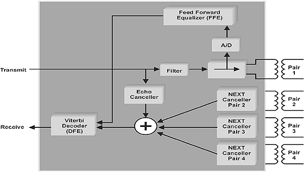
1000Base-T receiver
4.4.11 1000BASE-TX
This version transmits over four pairs of cable, two pairs in each direction of transmission (as opposed to all the four, for 1000Base-T over Cat5). Its simplified design has reduced the cost of required electronics. Since it does not carry out two-way transmission, crosstalk between the cables is significantly reduced, and encoding is relatively simple. 1000Base-TX will only operate over Cat6.

1000BASE-TX
4.4.12 Gigabit Ethernet Buffered Distributors
Gigabit Ethernet nodes can be connected to switches, or to less expensive full-duplex repeaters, also referred to as Buffered Distributors. As shown in Figure 4.10, these devices have a basic MAC function in each port, which enables them to verify that a complete frame is received and compute its frame check sequence (FCS) to verify the frame validity. Then the frame is buffered in the internal memory of the port before being forwarded to the other ports of the switch. Thus it combines the functions of a repeater with some features of a switch.

Gigabit Ethernet full-duplex repeaters
All ports on the device operate at the same speed of 1 Gbps, and in full-duplex mode so it can simultaneously send and receive from any port. The repeater uses IEEE802.3x flow control to ensure that the small internal buffers associated with each port do not overflow. When the buffers are filled to a critical level, it tells the transmitting node to stop sending until the buffers have been sufficiently emptied.
4.5 Gigabit Ethernet design considerations
The maximum cable distances that can be used between the node and a full-duplex 1000Base-SX and LX switch depend mainly on the chosen wavelength, the type of cable, and its bandwidth. The maximum transmission distances on multimode cable are limited by the Differential Mode Delay (DMD). The very narrow beam of laser light injected into the multimode fiber results in a relatively small number of rays going through the fiber core. These rays each have different propagation times because they are going through differing lengths of glass by zigzagging through the core to a greater or lesser extent. This can cause jitter and interference at the receiver. The problem is overcome by using a conditioned launch of the laser into the multimode fiber. This spreads the laser light evenly over the core of the multimode fiber so the laser source looks more like a Light Emitting Diode (LED) source, resulting in smoother spreading of the pulses and less interference. This conditioned launch is done in the 1000Base-SX transceivers.
The following table gives the maximum distances for full-duplex 1000Base-X switches.
Maximum fiber distances for 1000Base-X (full-duplex)

Learning objectives
When you have completed study of this chapter you should be able to:
- Describe the origins of TCP/IP
- Compare the OSI and DARPA (DoD) models
- Describe the overall structure of the TCP/IP protocol suite
5.1 The origins of TCP/IP
In the early 1960s The US Department of Defense (DoD) indicated the need for a wide-area communication system, covering the United States and allowing the interconnection of heterogeneous hardware and software systems.
In 1969 The Advanced Research Projects Agency (ARPA) contacted a small private company by the name of Bolt, Barenek and Newman (BBN) to assist with the development of the protocols. Other participants in the project included the University of Berkeley (California) Development work commenced in 1970 and by 1972 approximately 40 sites were connected via TCP/IP. In 1973 the first international connection was made and in 1974 TCP/IP was released to the public.
Initially the network was used to interconnect US government, military and educational sites together. Slowly, as time progressed, commercial companies were allowed access and by 1990 the backbone of the Internet, as it was now known, was being extended into one country after the other.
One of the major reasons why TCP/IP has become the de facto standard world-wide for industrial and telecommunications applications is the fact that the Internet was designed around it in the first place and that, without it, no Internet access is possible.
5.2 The ARPA model vs the OSI model
Whereas the OSI model was developed in Europe by the International Organization for Standardization (ISO), the ARPA model (also known as the DoD or Department of Defense model) was developed in the USA by ARPA. Although they were developed by different bodies and at different points in time, both serve as models for a communications infrastructure and hence provide ‘abstractions’ of the same reality. The remarkable degree of similarity is therefore not surprising.
Whereas the OSI model has 7 layers, the ARPA model has 4 layers. The OSI layers map onto the ARPA model as follows:
- The OSI Session, Presentation and Application layers are contained in the ARPA Process/Application layer (also referred to simply as the Application layer)
- The OSI Transport layer maps onto the ARPA Host-to-Host layer (also referred to as the Host layer)
- The OSI Network layer maps onto the ARPA Internet layer
- The OSI Physical and Data Link layers map onto the ARPA Network Interface layer
The relationship between the two models is depicted in Figure 5.1.
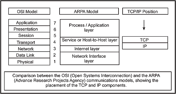
OSI vs ARPA models
5.3 The TCP/IP protocol suite vs the ARPA model
TCP/IP (or rather; the TCP/IP protocol suite) is not limited to the TCP and IP protocols, but consist of a multitude of interrelated protocols that occupy the upper three layers of the ARPA model. With the exception of the Point-to-Point Protocol (PPP) which resides in the upper half of the Network Interface Layer, the TCP/IP suite generally does not include the Network Interface layer, but merely depends on it for access to the medium.
5.3.1 The Network Interface layer
The Network Interface layer is responsible for transporting frames between hosts on the same physical network. It is implemented in the Network Interface Card or NIC, using hardware and firmware (i.e. software resident in Read Only Memory).
The NIC employs the appropriate medium access control methodology, such as CSMA/CA, CMSA/CD, token passing or polling, and is responsible for placing the data received from the upper layers within a frame before transmitting it. The frame format is dependent on the system being used, for example Ethernet or Frame Relay, and holds the hardware address of the source and destination hosts as well as a checksum for data integrity.
RFCs that apply to the Network Interface layer include:
- Asynchronous Transfer Mode (ATM), described in RFC 1438
- Switched Multi-megabit Data Service (SMDS), described in RFC 1209
- Ethernet, described in RFC 894,
- ARCNet, described in RFC 1201
- Frame Relay, described in RFC 1490
- Fiber Distributed Data Interface (FDDI), described in RFC 1103
Generally speaking, the TCP/IP suite does not cover the Network Interface layer since there is a multitude of technologies (such a those listed above) that ‘can do the job’. Notable exceptions in this regard are:
- Serial Line Internet Protocol (SLIP), described in RFC 1055
- Point-to-Point Protocol (PPP), described in RFC 1661
Both SLIP and PPP are essentially (OSI) Data Link layer protocols, thus they occupy only the upper half of the TCP/IP Network Interface layer. Both are used to carry IP datagrams over telephone lines, but SLIP has largely been phased out in favor of PPP.
Note: Any Internet-related specification is originally submitted as a request for comments or RFC. As time progresses an RFC may become a standard, or a recommended practice, and so on. Regardless of the status of an RFC, it can be obtained from various sources on the Internet such as http://www.rfc-editor.org.
5.3.2 The Internet layer
This layer is primarily responsible for the routing of packets from one host to another. The emphasis is on ‘packets’ as opposed to frames, since at this level the data has not yet been placed in a frame for transmission. Each packet contains the address information needed for its routing through the Internet work to the receiving host.
The dominant protocol at this level is the Internet Protocol (IP).
There are, however, several other protocols required at this level. These protocols include:
- Address Resolution Protocol (ARP), RFC 826. This is a protocol used for the translation of an IP address to a hardware (MAC) address, such as required by Ethernet.
- Reverse Address Resolution Protocol (RARP), RFC 903. This is the complement of ARP and translates a hardware address to an IP address.
- Internet Control Message Protocol (ICMP), RFC 792. This is a protocol used for sending control or error messages between routers or hosts. One of the best-known applications here is the ‘ping’ or ‘echo request’ used to test a communications link.
5.3.3 The Host-to-Host layer
This layer is primarily responsible for data integrity between the sender host and receiver host regardless of the path or distance used to convey the message. Communications errors are detected and corrected at this level.
It has two protocols associated with it, these being:
- User Data Protocol (UDP). This is a connectionless (unreliable) protocol used for higher layer port addressing. It offers minimal protocol overhead and is described in RFC 768
- Transmission Control Protocol (TCP). This is a connection-oriented protocol that offers vastly improved protection and error control. This protocol, the TCP component of TCP/IP, is the heart of the TCP/IP suite of applications. It provides a very reliable method of transferring data in byte (octet) format, between applications. This is described in RFC 793.
5.3.4 The Application layer
This layer provides the user or application programs with interfaces to the TCP/IP stack. At this level there are many protocols used, some of the more common ones being:
- File Transfer Protocol (FTP), which as the name implies, is used for the transfer of files between hosts using TCP. It is described in RFC 959
- Trivial File Transfer Protocol (TFTP), which is an ‘economical’ version of FTP and uses UDP instead of TCP for reduced overhead. It is described in RFC 783
- Simple Mail Transfer Protocol (SMTP), which is an example of an application that provides access to the TCP and IP for programs sending e-mail. It is described in RFC 821
- TELNET (TELecommunications NETwork), which is used to emulate terminals and for remote access to servers. It can, for example, emulate a VT100 terminal across a network
Other protocols at this layer include POP3, RPC, RLOGIN, IMAP, HTTP and NTP. Users can also develop their own Application layer protocols by means of developers’ toolkits.
The TCP/IP suite is shown in Figure 5.2 on the following page:

The TCP/IP protocol suite
Learning objectives
When you have completed the study of this chapter, you should be able to:
- Explain the basic operation of all Internet layer protocols including IP, ARP, RARP and ICMP
- Explain the purpose and application of the different fields in the IPv4 header
- Invoke APv4, ARP and ICMP, capture their headers with a protocol analyzer and compare the headers with those in the notes. You should be able to interpret the fundamental operations taking place and verify the different fields in each header
- Demonstrate the fragmentation capability of IPv4 using a protocol analyzer
- Explain the differences between historical class A, B and C addresses, and the relationship between NetID and HostID
- Explain the concept of classless addressing and CIDR
- Explain the concept of subnet masks and prefixes
- Explain the concept of subnetting by means of an example
- Explain, in very basic terms, the concept of supernetting
- Set up hosts in terms of IP addresses, subnet masks and default gateways
- Understand the principles of routing, the difference between interior and exterior gateway protocols, name some examples of both and explain, in very basic terms, their principles of operation
- Explain the basic concepts of IPv6
6.1 Overview
As pointed out in the previous chapter, the Internet layer is not populated by a single protocol, but rather by a collection of protocols.
They include:
- The Internet Protocol (IP)
- The Internet Control Message Protocol (ICMP),
- The Address Resolution Protocol (ARP),
- The Reverse Address Resolution Protocol (RARP), and
- Routing protocols (such as RIP, OSPF, BGP-4, etc)
6.2 IPv4
IP is at the core of the TCP/IP suite. It is primarily responsible for routing packets towards their destination, from sending host to receiving host via multiple routers. This task is performed on the basis of the IP addresses embedded in the header of each IP datagram.
The most prevalent version of IP in use today is version 4 (IPv4), which uses a 32-bit address. However, because of an ever increasing demand for IP addresses, IPv4 is being replaced by version 6 (IPv6 or IPng), which uses a 128-bit address.
This chapter will focus primarily on version 4 as a vehicle of explaining the fundamental processes involved, but will also provide an introduction to version 6.
6.2.1 Source of IP addresses
The ultimate control over IP addresses is vested in ICANN, the Internet Corporation for Assigned Names and Numbers. This was previously the task of IANA, the Internet Assigned Numbers Authority. This responsibility is, in turn, delegated to the five Regional Internet Registries (RIRs).
They are:
- APNIC: Asia-Pacific Network Information Center (www.apnic.net)
- ARIN: American Registry for Internet Numbers (/www.arin.net)
- RIPE NCC: Reseau IP Europeens (/www.ripe.net)
- AfriNIC: African Network Information Centre (www.afrinic.org)
- LACNIC: Latin American and Caribbean Registry or ‘Registro de Direcciones de Internet para American Latina y Cariba’ (www.lacnic.net)
The RIRs allocate blocks of IP addresses to Internet Service Providers (ISPs) under their jurisdiction, for subsequent issuing to users or sub-ISPs.
The use of ‘legitimate’ IP addresses is a prerequisite for connecting to the Internet. For systems not connected to the Internet, any IP addressing scheme may be used. It is, however, recommended that so-called ‘private’ Internet addresses are used for this purpose, as outlined in this chapter.
6.2.2 The purpose of the IP address
The MAC or hardware address discussed earlier is unique for each node, and has been allocated to that particular node e.g. NIC at the time of its manufacture. The equivalent for a human being would be an ID or Social Security number. As with a human ID number, the MAC address belongs to that node and follows it wherever it goes. This number works fine for identifying hosts on a LAN where all nodes can ‘see’ (or rather, ‘hear’) each other.
With human beings the problem arises when the intended recipient is living in another city, or worse, in another country. In this case the ID number is still relevant for final identification, but the message (e.g. a letter) first has to be routed to the destination by the postal system. For the postal system, a name on the envelope has little meaning. It requires a postal address.
The TCP/IP equivalent of this postal address is the IP address. As with the human postal address, this IP address does not belong to the node, but rather indicates its place of residence. For example, if an employee has a fixed IP address at work and he resigns, he will leave his IP address behind and his successor will ‘inherit’ it.
Since each host (which already has a MAC or hardware address) needs an IP address in order to communicate across the Internet, resolving host MAC addresses versus IP addresses is a mandatory function. This is performed by the Address Resolution Protocol (ARP), which is to be discussed later on in this chapter.
6.2.3 IPv4 address notation
The IPv4 address consists of 32 bits, e.g.
11000000011001000110010000000001
Since this number is fine for computers but a little difficult for human beings, it is divided into four octets, which for ease of reference could be called w, x, y and z. Each octet is then converted to its decimal equivalent.

IP address structure
The result of the conversion is written as 192.100.100.1 and is known as the ‘dotted decimal’ or ‘dotted quad’ notation.
6.2.4 Network ID and Host ID
Consider the following postal address:
- 4 Kingsmill Street
- Claremont WA 6010
- Australia
The first line, 4 Kingsmill Street, enables the local postal deliveryman at the Australia Post office in Claremont (Perth), Western Australia (postal code 6010) to deliver a letter to that specific residence. This assumes that the letter has already found its way to the Claremont post office from wherever it was posted. The second part of the address enables the postal system to route the letter towards its destination post office from anywhere in the world.
In similar fashion, an IP address has two distinct parts. The first part, the Network ID (NetID) is a unique number identifying a specific network and allows IP routers to forward a packet towards its destination network from anywhere in the world, provided there is a network connection between sender and recipient. The second part, the HostID (HostID) is a number allocated to a specific machine (host) on the destination network and allows the router servicing that host to deliver the packet directly to the host.
For example, in the IP address 192.100.100.5, the computer number or HostID could be 5, and it would be connected to NetID 192.100.100. The number of the network itself would be written as 192.100.100.0.
6.2.5 Address classes
Originally the intention was to allocate IP addresses in so-called address classes. Although the system proved to be problematic and was consequently abandoned with the result that IP addresses are currently issued ‘classless’, the legacy of IP address classes remains and has to be understood.
To provide for flexibility in assigning addresses to networks, the interpretation of the address field was coded to specify either:
- A small number of networks with a large number of hosts (class A)
- A moderate number of networks with a moderate number of hosts (class B),
- A large number of networks with a small number of hosts (class C)
In addition, there was provision for extended addressing modes: class D was reserved for multicasting whilst E was reserved for future use.
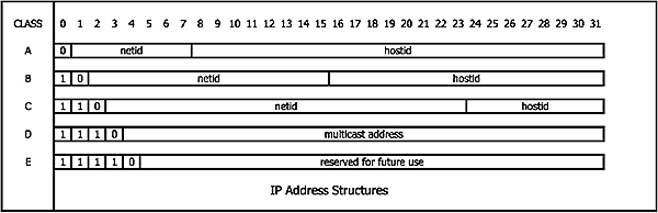
IPv4 address classes
- For class A, the first bit is fixed as ‘0’
- For class B the first 2 bits are fixed as ‘10’
- For class C the first 3 bits are fixed as ‘110’
6.2.6 Determining the address class by inspection
The NetID should normally not be all ‘0’s as this indicates a local network. With this in mind, analyze the first octet (‘w’).
For class A, the first bit is fixed at 0. The binary values for ‘w’ can therefore only vary between 000000002 (010) and 011111112 (12710). 0 is not allowed. However, 127 is also a reserved number, with 127.x.y.z reserved for loop-back testing whereby a host sends messages to itself, but bypassing layers 1 and 2 of the stack. 127.0.0.1 is the IP address most commonly used for this. The values for ‘w’ can therefore only vary between 1 and 126, which allows for 126 possible class A NetIDs.
For class B, the first two bits are fixed at 10. The binary values for ‘w’ can therefore only vary between 100000002 (12810) and 101111112 (19110).
For class C, the first three bits are fixed at 110. The binary values for ‘w’ can therefore only vary between 110000002 (19210) and 110111112 (22310).
The relationship between ‘w’ and the address class can therefore be summarized as follows.

IPv4 address range vs. class
6.2.7 Number of networks and hosts per address class
There are always two reserved host numbers, irrespective of class. These are ‘all zeros’ or ‘all ones’ for HostID. An IP address with a host number of zero is used as the address of the whole network. For example, on a class C network with the NetID = 200.100.100, the IP address 200.100.100.0 indicates the whole network. If all the HostID bits are set to 1, for example 200.100.100.255, then it means ‘all hosts on network 200.100.100.0’.
For class A, the number of NetIDs is determined by octet ‘w’. Unfortunately, the first bit (fixed at 0) is used to indicate class A and hence cannot be used. This leaves seven usable bits. Seven bits allow 27 = 128 combinations, from 0 to 127. 0 and 127 are reserved; hence only 126 NetIDs are possible. The number of HostIDs, on the other hand, is determined by octets ‘x’, ‘y’ and ‘z’. From these 24 bits, 224 = 16 777 218 combinations are available. All zeros and all ones are not permissible, which leaves 16 777 216 usable combinations.
For class B, the number of NetIDs is determined by octets ‘w’ and ‘x’. The first bits (10) are used to indicate class B and hence cannot be used. This leaves fourteen usable bits. Fourteen bits allow 214 = 16 384 combinations. The number of HostIDs is determined by octets ‘y’ and ‘z’. From these 16 bits, 216 = 65 536 combinations are available. All zeros and all ones are not permissible, which leaves 65,534 usable combinations.
For class C, the number of NetIDs is determined by octets ‘w’, ‘x’ and ‘y’. The first three bits (110) are used to indicate class C and hence cannot be used. This leaves twenty-two usable bits. Twenty-two bits allow 222 = 2 097 152 combinations. The number of HostIDs is determined by octet ‘z’. From these 8 bits, 28 = 256 combinations are available. Once again, all zeros and all ones are not permissible which leaves 254 usable combinations.

Hosts and subnets per class
6.2.8 Subnet masks
Strictly speaking, one should be referring to ‘netmask’ but the term ‘subnet mask’ is commonly used.
For routing purposes it is necessary for a device to strip the HostID off a destination IP address in order to ascertain whether or not the remaining NetID portion of the IP address matches its own network address.
Whilst it is easy for human beings, it is not the case for a computer and the latter has to be ‘shown’ which portion is NetID, and which is HostID. This is done by defining a subnet mask in which a ‘1’ is entered for each bit that is part of NetID, and a ‘0’ for each bit that is part of HostID. The computer takes care of the rest. The ‘1’s start from the left and run in a contiguous block.
For example: A conventional class C IP address, 192.100.100.5, written in binary, would be represented as 11000000 01100100 01100100 00000101. Since it is a class C address, the first 24 bits represent NetID and would therefore be indicated by ‘1’s. The subnet mask would therefore be:
11111111 11111111 1111111 00000000.
To summarize:
- IP address: 01100100 01100100 01100100 00000101
- Subnet mask: 11111111 11111111 11111111 00000000
|< NetID >| |< HostID>|
The mask, written in decimal dotted notation, becomes 255.255.255.0. This is the so-called default subnet mask for class C. Default subnet masks for classes A and B can be configured in the same manner.

Default netmasks
At present IP addresses are issued classless, which means that it is not possible to determine the boundary between NetID and HostID by analyzing the IP address itself. This makes the use of a subnet mask even more necessary.
Subnet masks can also be represented with ‘forward slash’ (/) after the IP address, followed by number of ‘1’s in the mask. A default class C address would therefore be written as 192.100.100.36/24. The /24 is called the prefix.
6.2.9 Subnetting
Assume that an organization based in Sydney has a block of 254 IP addresses, originally issued as a block of Class C addresses (192.100.100.0). It now wishes to open branch offices in Brisbane, Cairns, Perth, Melbourne and Adelaide. For this it would need a total of 6 NetIDs alone. For certain types of ‘cloud’ connections it would also require NetIDs for each point-to-point connection e.g. leased line. For the time being, we will ignore the ‘cloud’ issue and focus on the branch offices only.
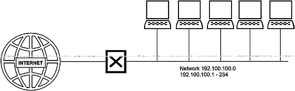
Before subnetting
The problem could be solved by creating subnetworks under the 192.100.100.0 network address and assigning a different subnetwork number to each LAN. To create a subnetwork, take some of the bits assigned to the HostID and use them for a subnetwork number, leaving fewer bits for HostID. Instead of NetID (24 bits) + HostID (8 bits), the IP address will now represent NetID (24 bits) + SubnetID (3 bits) + HostID (5 bits). To calculate the number of bits to be reassigned from HostID to SubnetID, choose a number of bits ‘n’ so that (2n) is bigger than or equal to the number of subnets required.
For most new routers all subnet numbers (including those consisting of all ‘0’s and all ‘1’s) can be used although it might have to be specifically enabled on the router. For older routers this is generally not possible, so two subnets are lost in the process and hence the number above needs to be modified to (2n)-2. In our case 6 subnets are required; so 3 bits have to be taken from the HostID since (23) = 8.
Note that the first subnet consisting of all zeros is called “subnet zero” and the last subnet made up of all 1s is called the “all-ones subnet”. The use of these subnets was originally discouraged due to possible confusion over having a network and subnet with the same address. This is only relevant today for legacy equipment which does not implement CIDR. All CIDR-compliant routing protocols transmit both length and suffix avoiding this problem.
Since only 5 bits are now available for HostID, each subnet can only have 30 HostIDs numbered 00001 (110) through 11110 (3010), since neither 00000 nor 11111 is allowed. To be technically correct, each subnetwork will only have 29 hosts since one HostID will be allocated to the router on that subnetwork. Note that the total available number of HostIDs has dropped from 254 to 240 (with 8 subnets having 30 hosts each).
The ‘z’ of the IP address is calculated by concatenating the SubnetID and the HostID.
For example, the network number for subnet 7 would have octet ‘z’ as 111 (SubnetID) concatenated with 00000 (HostID = ‘this network’), resulting in 224. The lowest assignable value for octet ‘z’ in subnet 7 would be 111 (SubnetID) concatenated with 00001 (HostID), resulting in 11100001 or 22510. In similar fashion the biggest assignable value would be 11111110 or 25410. The IP addresses on subnet 7 (192.100.100.224) would therefore range between 192.100.100.225 and 192.100.100.254 as shown in Figure 6.7.

IPv4 address allocation – 8 subnets on class C address
In the preceding example, the first 3 bits of the HostID have been allocated as SubnetID, and have therefore effectively become part of the NetID. A default class C subnet mask would unfortunately obliterate these 3 bits, with the result that the local routers would not be able to route messages between the subnets. For this reason the subnet mask has to be extended by another 3 bits to the right, so that it becomes 11111111 11111111 11111111 11100000. The extra bits have been typed in italics, for clarity. The subnet mask for all hosts is now 255.255.255.224 or /27.

After subnetting
6.2.10 VLSM
In the preceding example the available HostIDs were divided into equally sized chunks. Although it is the simplest approach, it is not always ideal since some subnets require more IP addresses than others. In our example there are 6 terrestrial links (leased lines) between the offices, which would require 7 subnets for the actual LANs and 6 for the links. However, the links only require 2 IP addresses each!
Provided that the routers support Variable Length Subnet Masking or VLSM, the problem could be solved by taking only one of the subnets (say subnet 7 i.e. 192.100.100.224/27) and subnetting it even further, using the same approach as before. For 6 links we need to take another 3 bits from subnet 7’s HostID and tack it onto the existing SubnetID. This will give 8 additional options to add on to the SubnetID, ranging from 000 to 111. The resulting HostID would now be only 2 bits long, but even though the ‘00’ and ‘11’ values cannot be used, there are still 2 usable values, which is sufficient.
Let us do some calculations for the first link (say Sydney-Melbourne). For octet ‘z’ in the network number we will use 000 to designate the link (one of the 8 options) and concatenate that with the existing 111, which results in 111000. Now concatenate that with a further 00 for HostID and the final result is 11100000 or 224. The network number for the Sydney-Melbourne link is thus 192.100.100.224/30. Note the extended subnet mask.
On this particular subnet, only two HostIDs are possible viz. 110 (012) and 210 (102) Octet ‘z’ would therefore be either 11100001 (225) or 11100010 (226). The IP addresses of the router ports attached to this link would therefore be 192.100.100.225/30 and 192.100.100.226/30.
6.2.11 Private vs Internet-unique IP addresses
If it is certain that a network will never be connected to the Internet, any IP address can be used as long as the IP addressing rules are followed. If there are fewer than 254 hosts on the network, it is easiest to use class C addresses. Assign each LAN segment its own class C NetID. Then assign each host a complete IP address simply by appending the dotted decimal HostID to the NetID.
If there is a possibility of connecting a network to the Internet, one should not use IP addresses that might result in address conflicts. In order to prevent such conflicts, obtain a set of Internet-unique IP addresses from an ISP or use IP addresses reserved for private works as described in RFC 1918.
ICANN has reserved several blocks of Private IP addresses for this purpose as shown below:

Reserved IP addresses
Reserved IP addresses are not routed on the Internet because Internet routers are programmed not to forward messages to or from these addresses.
A private network can easily be connected to the Internet by means of a router capable of performing Network Address Translation (NAT). The NAT router then translates the private addresses to one or more legitimate Internet addresses. An added advantage of this approach is that the private addresses are invisible to the outside world. This, plus the fact that most NAT routers have built-in firewalls, makes it a safe approach.
6.2.12 Classless addressing
Initially, the IPv4 Internet addresses were only assigned in classes A, B and C. This approach turned out to be extremely wasteful, as large amounts of allocated addresses were not being used. Not only was the class D and E address space underutilized, but a company with 500 employees that was assigned a class B address would have 65,034 addresses that no-one else could use.
At present IPv4 addresses are considered classless. The issuing authorities (ICANN, through the five RIRs) simply hand down a block of contiguous addresses to ISPs, who can then issue them one by one, or break the large block up into smaller blocks for distribution to sub-ISPs, who will then repeat the process. Because of the fact that the 32 bit IPv4 addresses are no longer considered ‘classful’, the traditional distinction between class A, B and C addresses and the implied boundaries between the NetID and HostID can be ignored. Instead, whenever an IPv4 network address is assigned to an organization, it is done in the form of a 32-bit network address and a corresponding 32-bit mask, usually expressed as a prefix.
6.2.13 Classless Inter-Domain Routing (CIDR)
In the early days of the Internet, IP addresses were allocated by the Network Information Center (NIC). At that stage this was done more or less at random and each address had to be advertised individually in the routing tables of the Internet routers.
Consider, for example, the case of following 4 private (‘traditional’ class C) networks, each one with its own contiguous block of 256 addresses, being serviced by one ISP:
- Network A: 200.100.0.0 (IP addresses 200.100.0.1–200.100.0.255)
- Network B: 192.33.87.0 (IP addresses 192.33.87.1–192.33.87.255)
- Network C: 194.27.11.0 (IP addresses 194.27.11.1–194.27.11.255)
- Network D: 202.15.16.0 (IP addresses 202.15.16.1–202.15.16.255)
If we ignore the reserved HostIDs (all ‘0’s and all ‘1’s), then the concentrating router at the ISP would have to advertise 4 × 256 = 1024 separate network addresses. In a real life situation, the ISP’s router would have to advertise tens of thousands of addresses. It would also be seeing hundreds of thousands, if not millions, of addresses advertised by the routers of other ISPs across the globe. In the early nineties the situation was so serious it was expected that, by 1994, the routers on the Internet would no longer be able to cope with the multitude of routing table entries.

Network advertising without CIDR
To alleviate this problem, the concept of Classless Inter-Domain Routing (CIDR) was introduced. Basically, CIDR removes the imposition of the class A, B and C address masks and allows the owner of a network to ‘supernet’ multiple addresses together. It then allows the concentrating router to aggregate (or ‘combine’) these multiple contiguous network addresses into a single route advertisement on the Internet.
Let us take the same example as before, but this time we allocate contiguous addresses. Note that ‘w’ can have any value between 1 and 255 since the address classes are no longer relevant.
| w x y z | |
| Network A: | 220.100.0. 0 |
| Network B: | 220.100.1. 0 |
| Network C: | 220.100.2. 0 |
| Network D: | 220.100.3. 0 |
CIDR now allows the router to advertise all 1024 network addresses under one advertisement, using the starting address of the block (220.100.0.0) and a CIDR (supernet mask) of 255.255.252.0. This is achieved as follows.
CIDR uses a mask similar to the one used for subnet masking, but it has fewer ‘1’s than the subnet mask. Whereas the 1s in the subnet mask indicate the bits that comprise the network ID, the ‘1’s in the CIDR (supernet) mask indicates the bits in the IP address that do not change. In the following example we will, for the sake of simplicity, include the HostIDs with all ‘1’s and all ‘0’s.
The total number of computers in this ‘supernet’ can be calculated as follows:
Number of ‘1’s in the subnet mask = 24
Number of hosts per network = (2(32-24) ) = 28 = 256
Number of ‘1’s in the CIDR mask = 22
X= (Number of ‘1’s in the subnet mask minus number of ‘1’s in the CIDR mask) = 2
Number of networks aggregated = 2X = 22 = 4
Total number of hosts = 4 × 256 = 1024
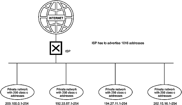
Network advertising with CIDR
The route advertisement of 220.100.100.0 mask 255.255.252.0 implies a supernet comprising 4 networks, each with 256 possible hosts. The lowest IP address is 220.100.100.1 and the highest is 220.100.3.254. The first mask in the following table (255.255.255.0) is the subnet mask while the second mask (255.255.252.0) is the CIDR mask.

Binary equivalents of IP addresses and masks used in this example
CIDR and the concept of classless addressing go hand in hand since it is obvious that the concept can only work if the ISPs are allowed to exercise strict control over the issuing and allocation of IP addresses. Before the advent of CIDR, clients could obtain IP addresses and regard it as their ‘property’. Under the new dispensation, the ISP needs to keep control over its allocated block(s) of IP addresses. A client can therefore only ‘rent’ IP addresses from an ISP and the latter may insist on its return, should the client decide to change to another ISP.
6.2.14 IPv4 header structure
The IP header is appended to the PDU that IP accepts from higher-level protocols, before routing it across the network. The IP header consists of six 32-bit ‘long words’ and is made up as follows:

IPv4 header
Ver: 4 bits
The version field indicates the version of the IP protocol in use, hence the format of the header. In this case it is 4.
IHL: 4 bits
IHL is the length of the IP header in 32 bit ‘long words’, and thus points to the beginning of the data. This is necessary since the IP header can contain options and therefore has a variable length. The minimum value is 5, representing 5 × 4 = 20 bytes.
Type of Service: 8 bits
The Type of Service (ToS) field is intended to provide an indication of the parameters of the quality of service desired. These parameters are used to guide the selection of the actual service parameters when transmitting a datagram through a particular network.
Some networks offer service precedence, which treats high precedence traffic as more important than other traffic (generally by accepting only traffic above a certain precedence at times of high load). The choice involved is a three-way trade-off between low delay, high reliability, and high throughput.

Type of service
The ToS field is composed of a 3-bit precedence field (which is often ignored) and an unused (LSB) bit that must be 0. The remaining 4 bits may only be turned on one at a time, and are allocated as follows:
- Bit 3: Minimize delay
- Bit 4: Maximize throughput
- Bit 5: Maximize reliability
- Bit 6: Minimize monetary cost
RFC 1340 (corrected by RFC 1349) specifies how all these bits should be set for standard applications. Applications such as TELNET and RLOGIN need minimum delay since they transfer small amounts of data. FTP needs maximum throughput since it transfers large amounts of data. Network management (SNMP) requires maximum reliability and Usenet news (NNTP) needs to minimize monetary cost.
Most TCP/IP implementations do not support the ToS feature, although some newer implementations of BSD and routing protocols such as OSPF and IS-IS can make routing decisions on it.
Total Length: 16 bits
This is the length of the datagram, measured in bytes, including the header and data. By using this field and the header length, it can be determined where the data starts and ends. This field allows the length of a datagram to be up to 216 = 65,536 bytes, the maximum size of the segment handed down to IP from the protocol above it.
Such long datagrams are, however, impractical for most hosts and networks. All hosts must at least be prepared to accept datagrams of up to 576 octets (whether they arrive whole or in fragments). It is recommended that hosts only send datagrams larger than 576 octets if they have the assurance that the destination is prepared to accept the larger datagrams.
The number 576 is selected to allow a reasonably-sized data block to be transmitted in addition to the required header information. For example, this size allows a data block of 512 octets plus 64 header octets to fit in a datagram, which is the maximum size permitted by X.25. A typical IP header is 20 octets, allowing some space for headers of higher-level protocols.
Identification: 16 bits
This number uniquely identifies each datagram sent by a host and is normally incremented by one for each datagram sent. In the case of fragmentation it is appended to all fragments of the same datagram for the sake of reconstructing the datagram at the receiving end. It can be compared to the ‘tracking’ number of an item delivered by registered mail or by courier.
Flags: 3 bits
There are two flags:
- The DF (Don’t Fragment) flag is set (=1) by the higher-level protocol (e.g. TCP) if IP is NOT allowed to fragment a datagram. If such a situation occurs, IP will not fragment and forward the datagram, but simply return an appropriate ICMP message to the sending host
- The MF (More Flag) is used as follows. If fragmentation DOES occur, MF=1 will indicate that there are more fragments to follow, whilst MF=0 indicates that it is the last fragment
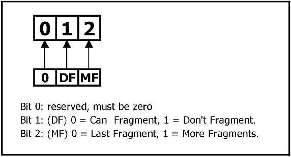
Flag structure
Fragment Offset: 13 bits
This field indicates where in the original datagram this fragment belongs. The fragment offset is measured in units of 8 bytes (64 bits). In other words, the transmitted offset value is equal to the actual offset divided by eight. This constraint necessitates fragmentation in such a way that the offset is always exactly divisible by eight. It had to be done this way since for large chunks of data (close to 64K) the offset value for the last fragment would be almost 64K, requiring a 16 bit field. However, three bits have been used for the Flags field and therefore the actual offset (in bytes) is divided by 23 = 8 as a precaution.
Time to Live: 8 bits
The purpose of this field is to cause undeliverable datagrams to be discarded. Every router that processes an IP datagram must decrease the TTL by one and if this field contains the value zero, then the datagram must be destroyed.
The original design called for TTL to be a timer function, but that is difficult to implement and currently all routers simply decrement TTL every time they pass a datagram.
Protocol: 8 bits
This field indicates the next (higher) level protocol used in the data portion of the IP datagram, in other words the protocol that resides above IP in the protocol stack and which has passed the datagram on to IP.
Typical values are 0x0806 for ARP and 0x8035 for RARP (0x meaning ‘hexadecimal’).
Header Checksum: 16 bits
This is a checksum on the header only, referred to as a ‘standard Internet checksum’. Since some header fields change (e.g. TTL), this is recomputed and verified at each point that the IP header is processed. It is not necessary to cover the data portion of the datagram, as the protocols making use of IP, such as ICMP, IGMP, UDP and TCP, all have a checksum in their headers to cover their own header and data.
To calculate it, the header is divided up into 16-bit words. These words are then added together (normal binary addition with carry) one by one, and the interim sum stored in a 32-bit accumulator. When done, the upper 16 bits of the result is stripped off and added to the lower 16 bits. If, after this, there is a carry over to the 17th bit, it is carried back and added to bit 0. The result is then truncated to 16 bits.
Source and Destination Address: 32 bits each
These are the 32-bit IP addresses of both the origin and the destination of the datagram.
6.2.15 Packet fragmentation
It should be clear by now that IP might often have difficulty in sending packets across a network since, for example, Ethernet can only accommodate 1500 octets at a time and X.25 is limited to 576. This is where the fragmentation process comes into play. The relevant field here is ‘fragment offset’ (13 bits) while the relevant flags are DF (don’t fragment) and MF (more fragments).
Consider a datagram consisting of an IP header followed by 3500 bytes of data. This cannot be transported over an Ethernet network, so it has to be fragmented in order to ‘fit’. The datagram will be broken up into three separate datagrams, each with their own IP header, with the first two frames around 1500 bytes and the last fragment around 500 bytes. The three frames will travel to their destination independently, and will be recognized as fragments of the original datagram by virtue of the number in the identifier field. However, there is no guarantee that they will arrive in the correct order, and the receiver needs to reassemble them.
For this reason the Fragment Offset field indicates the distance or offset between the start of this particular fragment of data, and the starting point of the original frame. One problem though – since only 13 bits are available in the header for the fragment offset (instead of 16), this offset is divided by 8 before transmission, and again multiplied by 8 after reception, requiring the data size (i.e. the offset) to be a multiple of 8 – so an offset of 1500 won’t do. 1480 will be OK since it is divisible by 8. The data will be transmitted as fragments of 1480, 1480 and finally the remainder of 540 bytes. The fragment offsets will be 0, 1480 and 2960 bytes respectively, or 0, 185 and 370 – after division by 8.
Incidentally, another reason why the data per fragment cannot exceed 1480 bytes for Ethernet, is that the IP header has to be included for each datagram (otherwise individual datagrams will not be routable) and hence 20 of the 1500 bytes have to be forfeited to the IP header.
The first frame will be transmitted with 1480 bytes of data, Fragment Offset = 0, and MF (more flag) = 1.
The second frame will be transmitted with the next 1480 bytes of data, Fragment Offset = 185, and MF = 1.
The last third frame will be transmitted with 540 bytes of data, Fragment Offset = 370, MF = 0.
Some protocol analyzers will indicate the offset in hexadecimal; hence it will be displayed as 0xb9 and 0x172, respectively.
For any given type of network the packet size cannot exceed the so-called MTU (Maximum Transmission Unit) for that type of network. The following are some typical values:
- Default 576 bytes
- Analog dialup (<128 kbps) 576 bytes
- xDSL 1500 bytes
- Ethernet 1500 bytes
The fragmentation mechanism can be checked by doing a ‘ping’ across a network, and setting the data (–l) parameter in the ping command to exceed the MTU value for the network.

IPv4 fragmentation
6.3 IPv6/IPng
6.3.1 Introduction
IPng (‘IP new generation’), as documented in RFC 1752, was approved by the Internet Engineering Steering Group in November 1994 and made a Proposed Standard. The formal name of this protocol is IPv6 (‘IP version 6’). After extensive testing, IANA gave permission for its deployment in mid-1999.
IPv6 is an update of IPv4, to be installed as a ‘backwards compatible’ software upgrade, with no scheduled implementation dates. It runs well on high performance networks such as ATM, and at the same time remains efficient enough for low bandwidth networks such as wireless LANs. It also makes provision for Internet functions such as audio broadcasting and encryption.
Upgrading to and deployment of IPv6 can be achieved in stages. Individual IPv4 hosts and routers may be upgraded to IPv6 one at a time without affecting any other hosts or routers. New IPv6 hosts and routers can be installed one by one. There are no pre-requisites to upgrading routers, but in the case of upgrading hosts to IPv6 the DNS server must first be upgraded to handle IPv6 address records.
When existing IPv4 hosts or routers are upgraded to IPv6, they may continue to use their existing address. They do not need to be assigned new IPv6 addresses; neither do administrators have to draft new addressing plans.
The simplicity of the upgrade to IPv6 is brought about through the transition mechanisms built into IPv6. They include the following:
- The IPv6 addressing structure embeds IPv4 addresses within IPv6 addresses, and encodes other information used by the transition mechanisms
- All hosts and routers upgraded to IPv6 in the early transition phase will be ‘dual’ capable (i.e. implement complete IPv4 and IPv6 protocol stacks)
- Encapsulation of IPv6 packets within IPv4 headers will be used to carry them over segments of the end-to-end path where the routers have not yet been upgraded to IPv6
The IPv6 transition mechanisms ensure that IPv6 hosts can inter-operate with IPv4 hosts anywhere in the Internet up until the time when IPv4 addresses run out, and allows IPv6 and IPv4 hosts within a limited scope to inter-operate indefinitely after that. This feature protects the huge investment users have made in IPv4 and ensures that IPv6 does not render IPv4 obsolete. Hosts that need only a limited connectivity range (e.g., printers) need never be upgraded to IPv6.
6.3.2 IPv6 overview
The changes from IPv4 to IPv6 fall primarily into the following categories:
- Expanded routing and addressing capabilities
IPv6 increases the IP address size from 32 bits to 128 bits, to support more levels of addressing hierarchy and a much greater number of addressable nodes, and simpler auto-configuration of addresses - Anycasting
A new type of address called an Anycast address is defined; to identify sets of nodes where a packet sent to the group of Anycast addresses is delivered to (only) one of the nodes. The use of Anycast addresses in the IPv6 source route allows nodes to control the path that their traffic flows - Header format simplification
Some IPv4 header fields have been dropped or made optional, to reduce the effort involved in processing packets. The IPv6 header was also kept as small as possible despite the increased size of the addresses. Even though the IPv6 addresses are four times longer than the IPv4 addresses, the IPv6 header is only twice the size of the IPv4 header - Improved support for options
Changes in the way IP header options are encoded allows for more efficient forwarding, less stringent limits on the length of options, and greater flexibility for introducing new options in the future - Quality-of-service capabilities
A new capability is added to enable the labeling of packets belonging to particular traffic ‘flows’ for which the sender requests special handling, such as special ‘quality of service’ or ‘real-time’ service - Authentication and privacy capabilities
IPv6 includes extensions that provide support for authentication, data integrity, and confidentiality
6.3.3 IPv6 header format

IPv6 header
The header contains the following fields:
Ver: 4 bits
The IP version number, viz. 6.
Traffic Class: 8 bits
This is used in conjunction with the Flow Label and indicates an Internet traffic priority delivery value.
Flow Label: 20 bits
A flow is a sequence of packets sent from a particular source to a particular (unicast or multicast) destination for which the source desires special handling by the intervening routers. This is an optional field to be used if specific non-standard (‘non-default’) handling is required to support applications that require some degree of consistent throughput in order to minimize delay and/or jitter. These types of applications are commonly described as ‘multi-media’ or ‘real-time’ applications.
The flow label will affect the way the packets are handled but will not influence the routing decisions.
Payload Length: 16 bits
The payload is the rest of the packet following the IPv6 header, in bytes. The maximum payload that can be carried behind a standard IPv6 header cannot exceed 65,536 bytes. With an extension header this is possible, and the datagram is then referred to as a Jumbo datagram. Payload Length differs slightly from the IPv4 ‘total length’ field in that it does not include the header length.
Next Header: 8 bits
This identifies the type of header immediately following the IPv6 header, using the same values as the IPv4 protocol field. Unlike IPv4, where this would typically point to TCP or UDP, this field could either point to the next protocol header (TCP) or to the next IPv6 extension header.

Header insertion and ‘next header’ field
Hop Limit: 8 bits
This is an unsigned integer, similar to TTL in IPv4. It is decremented by 1 by each node that forwards the packet. The packet is discarded if hop limit is decremented to zero.
Source IP Address: 128 bits
This is the IPv6 address of the initial sender of the packet.
Destination IP address: 128 bits
This is IPv6 Address of the intended recipient of the packet, which is not necessarily the ultimate recipient, if an optional routing header is present.
6.3.4 IPv6 extensions
IPv6 includes an improved option mechanism. Instead of placing extra option bytes within the main header, IPv6 options are placed in separate extension headers that are located between the IPv6 header and the Transport layer header in a packet.
Most IPv6 extension headers are not examined or processed by routers along a packet’s path until it arrives at its final destination. This leads to a major improvement in router performance for packets containing options. In IPv4 the presence of any options requires the router to examine all options.
IPv6 extension headers can be of arbitrary length and the total amount of options carried in a packet is not limited to 40 bytes as with IPv4. They are also not carried within the main header, as with IPv4, but are only used when needed, and are carried behind the main header. This feature, plus the manner in which they are processed, permits IPv6 options to be used for functions that were not practical in IPv4. Examples of this are the IPv6 authentication and security encapsulation options.
In order to improve the performance when handling subsequent option headers and the transport protocol which follows, IPv6 options are always an integer multiple of 8 bytes long in order to retain this alignment for subsequent headers.
The recommended sequence of headers in an IPv6 packet per RFC 2460 is:
- IPv6 header (40 bytes)
- Hop-by-hop options header (variable)
- Destination options header (1) (variable)
- Routing header (variable)
- Fragment header (variable)
- Authentication header (variable)
- Encapsulation Security Payload header (variable)
- Destination options header (2) (variable)
- Upper-layer header (e.g. TCP)

Carrying IPv6 extension headers
6.3.5 IPv6 addresses
IPv6 addresses are 128 bits long and are identifiers for individual interfaces or sets of interfaces. IPv6 Addresses of all types are assigned to interfaces (i.e. NICs) and NOT to nodes i.e. hosts. Since each interface belongs to a single node, any of that node’s interfaces’ unicast addresses may be used as an identifier for the node. A single interface may be assigned multiple IPv6 addresses of any type.
There are three types of IPv6 addresses. These are unicast, anycast, and multicast.
- Unicast addresses identify a single interface
- Anycast addresses identify a set of interfaces such that a packet sent to an Anycast address will be delivered to (any) one member of the set
- Multicast addresses identify a group of interfaces, such that a packet sent to a multicast address is delivered to all of the interfaces in the group. There are no broadcast addresses in IPv6, their function being superseded by multicast addresses
The IPv6 address is four times the length of IPv4 addresses (128 vs 32). This is 4 billion times 4 billion (296) times the size of the IPv4 address space. This works out to be 340,282,366,920,938,463,463,374,607,431,768,211,456. Theoretically this is approximately 665,570,793,348,866,943,898,599 addresses per square meter of the surface of the Earth (assuming the Earth’s surface is 511,263,971,197,990 square meters). In more practical terms, considering that the creation of addressing hierarchies will reduce the efficiency of the usage of the address space, IPv6 is still expected to support between 8×10¹⁷ to 2×1033 nodes. Even the most pessimistic estimate provides around 1500 addresses per square meter of the surface of the Earth.
IPv6 addresses are written in hexadecimal rather than the IPv4 dotted decimal notation. Each cluster of 4 characters is truncated with a colon (‘:’) sign. This results in an address such as 1234:5678:DEF0:1234:5678:0000:0000:9ABC. The ‘0000’ can be expressed as a single ‘0’, i.e. 1234:5678:DEF0:1234:5678:0:0:9ABC. Alternatively the entire string of ‘0’s can be written as ::, which results in 1234:5678:DEF0:1234:5678::9ABC.
IPv6 addresses are allocated to ‘groups’ of addresses used for specific purposes. For example, all addresses starting with the bits 001 (a total of 1/8 of the overall address space) have been allocated as Global Unicast addresses and those starting with 1111 1110 10 (a total of 1/1024 of the total address space) have been allocated as Link-local Unicast addresses. These leading bits were initially called the Format Prefix but the concept of formal Format Prefixes was deprecated in RFC3513. The bits are still there, though they are just not called anything. Global Unicast Addresses therefore start with the binary sequence 001x xxxx xxxx xxxx etc. This is written as 2000::/3, meaning that the first three bits (001) designate a Global Unicast Address and the rest can be anything.
There are several forms of unicast address assignment in IPv6. These are:
- Global Unicast addresses
- Unspecified addresses
- Loopback addresses
- IPv4-based addresses
- Link Local addresses
Site-local addresses were initially included in this list, but deprecated in September 2004.
Global Unicast addresses
These addresses are used for global communication. They are similar in function to IPv4 addresses under CIDR. Their format is:

Address format: Global Unicast address
The original format included a TLA (Top Level Aggregator), NLA (Next Level Aggregator) and SLA (Site Level Aggregator) but this approach has been deprecated in 1994.
Prefix: 48 bits
The first three bits are always 001, i.e. 2000:/3. The Prefix is the network ID used for routing to a particular site and is similar to the IPv4 NetID, although the composition of the number is more complex and indicates the hierarchy of service providers from the Internet backbone down to the user’s site.
Subnet ID: 16bits
This identifies a subnet within a site.
Interface ID: 64 bits
This is the unique identifier for a particular interface (e.g. a host). It is unique within the specific prefix and subnet and is the equivalent of the ‘HostID’ in IPv4. However, instead of an arbitrary number it would consist of the hardware address of the interface, e.g. the Ethernet MAC address in the IEEE EUI-64 format
Existing 48-bit MAC addresses are converted to the EUI-64 format by splitting them in the middle and inserting the string FF-FE in between the two halves.

Converting a 48-bit MAC address to EUI-64 format
Unspecified addresses
This can be written as 0:0:0:0:0:0:0:0, or simply :: (double colon). This address can be used as a source address by a station that has not yet been configured with an IP address. It can never be used as a destination address. This is similar to 0.0.0.0 in IPv4.
Loopback addresses
The loopback address 0:0:0:0:0:0:0:1 can be used by a node to send a datagram to itself. It is similar to the 127.0.0.1 of IPv4.
IPv4-based addresses
It is possible to construct an IPv6 address out of an existing IPv4 address. This is done by prepending 96 zero bits to an IPv4 address. The result is written as 0:0:0:0:0:0:192.100.100.3, or simply ::192.100.100.3.
Link-local unicast addresses
Stations that are not yet configured with either a provider-based address or a site local address may use link local addresses. Link-local addresses start with 1111 1110 10 i.e. FE80::/10. These addresses can only be used by stations connected to the same local network and packets addressed in this way cannot traverse a router, since there is no routing information contained within the header.

Link-local unicast addresses
Anycast addresses
An IPv6 Anycast address is an address that is assigned to more than one interface (typically belonging to different nodes), with the property that a packet sent to an Anycast address is routed to the ‘nearest’ interface having that address, according to the routing protocols’ measure of distance. Anycast addresses, when used as part of a route sequence, permits a node to select which of several internet service providers it wants to carry its traffic. This capability is sometimes called ‘source selected policies’. This would be implemented by configuring Anycast addresses to identify the set of routers belonging to ISPs (e.g. one Anycast address per ISP). These Anycast addresses can be used as intermediate addresses in an IPv6 routing header, to cause a packet to be delivered via a particular provider or sequence of providers.
Other possible uses of Anycast addresses are to identify the set of routers attached to a particular subnet, or the set of routers providing entry into a particular routing domain. Anycast addresses are allocated from the unicast address space, using any of the defined unicast address formats. Thus, Anycast addresses are syntactically indistinguishable from Unicast addresses. When a Unicast address is assigned to more than one interface, it ‘automatically’ turns it into an Anycast address. The nodes to which the address is assigned must be explicitly configured to know that it is an Anycast address.
Multicast addresses
IPv6 multicast addresses (FF00:/8) are identifiers for groups of interfaces. An interface may belong to any number of multicast groups. Multicast addresses have the following format:

Address format: IPv6 multicast
-
- FLAGS. Four bits are reserved for flags. The first 3 bits are currently reserved, and set to 0. The last bit (the least significant bit) is called T for ‘transient’. T = 0 indicates a permanently assigned (‘well-known’) multicast address, assigned by ICANN, while T = 1 indicates a non-permanently assigned (‘transient’) multicast address
- SCOPE is a 4-bit multicast scope value used to limit the scope of the multicast group, for example to ensure that packets intended for a local videoconference are not spread across the Internet.
The values are:
| 0 | Reserved | |
| 1 | Node-local | scope |
| 2 | Link-local | scope |
| 5 | Site-local | scope |
| 8 | Organization-local | scope |
| 14 | Global scope | |
| 15 | Reserved |
- MULTICAST GROUP ID defines a particular multicast group, either permanent or transient, within a given scope level. Permanent group IDs are assigned by ICANN.
The following example shows how it all fits together. The multicast address FF:08::43 points to all NTP servers in a given organization, in the following way:
- FF indicates that this is a multicast address
- 0 indicates that the T flag is set to 0, i.e. this is a permanently assigned multicast address
- 8 points to all interfaces in the same organization as the sender (see SCOPE options above)
- Group ID = 43 has been permanently assigned to network time protocol (NTP) servers
6.4 ARP
The Address Resolution Protocol (ARP) is used with IPv4. Initially the designers of IPv6 assumed that it would use ARP as well, but subsequent work by the SIP, SIPP and IPv6 working groups led to the development of the IPv6 ‘neighbor discovery’ procedures that encompass ARP, as well as those of router discovery.
Some network technologies make address resolution difficult. Ethernet NICs, for example, come with built-in 48-bit hardware (MAC) addresses. This creates several difficulties:
- There is no direct correlation between MAC addresses and IP addresses
- When the NIC is replaced the IP address then has to be remapped to a different MAC address
- The MAC address is too long to be encoded into the 32-bit IP address
To overcome these problems in an efficient manner, and eliminate the need for applications to know about MAC addresses, the Address Resolution Protocol (ARP) (RFC 826) resolves addresses dynamically.
When a host wishes to communicate with another one on the same physical network, it needs the destination MAC address in order to compose the basic layer 2 frame. If it does not know what the destination MAC address is, but has the IP address, it invokes ARP, which broadcasts a special type of datagram in order to resolve the problem. This is called an ARP request. This datagram requests the owner of the unresolved IP address to reply with its MAC address. All hosts on the local network will receive the broadcast, but only the one that recognizes its own IP address will respond.
While the sender could, of course, just broadcast the original message to all hosts on the network, this would impose an unnecessary load on the network, especially if the datagram was large. A small ARP request, followed by a small ARP reply, followed by a unicast transmission of the original datagram, is a much more efficient way of resolving the problem.
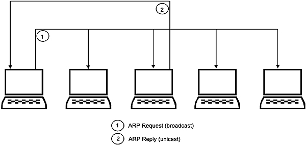
ARP operation
6.4.1 Address resolution cache
Because communication between two computers usually involves transfer of a succession of datagrams, it is prudent for the sender to ‘remember’ the MAC information it receives, at least for a while. Thus, when the sender receives an ARP reply, it stores the MAC address as well as the corresponding IP address in its ARP cache. Before sending any message to a specific IP address it checks first to see if the relevant address binding is in the cache. This saves it from repeatedly broadcasting identical ARP requests.
The ARP cache holds 4 fields of information for each device:
- IF index – Interface Index; the number of the entry in the table
- Physical address – the MAC address of the device
- Internet protocol (IP) address – the corresponding IP address
- Type – the type of entry in the ARP cache. There are 4 possible types:
4 = static – the entry will not change
3 = dynamic – the entry can change
2 = the entry is invalid
1 = none of the above
6.4.2 The ARP header
The layout of an ARP datagram is as follows:

ARP header
Hardware Type: 16 bits
Specifies the hardware interface type of the target, e.g.:
1 = Ethernet
3 = X.25
4 = Token ring
6 = IEEE 802.x
7 = ARCnet
Protocol Type: 16 bits
Specifies the type of high-level protocol address the sending device is using. For example,
204810 (0x800): IP
205410 (0x0806): ARP
328210 (0x8035): RARP
HA Length: 8 bits
The length, in bytes, of the hardware (MAC) address. For Ethernet it is 6.
PA Length: 8 bits
The length, in bytes, of the internetwork protocol address. For IP it is 4.
Operation: 8 bits
Indicates the type of ARP datagram:
1 = ARP request
2 = ARP reply
3 = RARP request
4 = RARP reply
Sender HA: 48 bits
The hardware (MAC) address of the sender, expressed in hexadecimal.
Sender PA: 32 bits
The (internetwork) protocol address of the sender. In the case of TCP/IP this will be the IP address, expressed in hexadecimal (not dotted decimal notation).
Target HA: 48 bits
The hardware (MAC) address of the target host, expressed in hexadecimal.
Target PA: 32 bits
The (internetwork) protocol (IP) address of the target host, expressed in hexadecimal.
Because of the use of fields to indicate the lengths of the hardware and protocol addresses, the address fields can be used to carry a variety of address types, making ARP applicable to a number of different network standards.
The broadcasting of ARP requests presents some potential problems. Networks such as Ethernet employ connectionless delivery systems i.e. the sender does not receive any feedback as to whether datagrams it has transmitted were received by the target device. If the target is not available, the ARP request destined for it will be lost without trace and no ARP response will be generated. Thus the sender must be programmed to retransmit its ARP request after a certain time period, and must be able to store the datagram it is attempting to transmit in the interim. It must also remember what requests it has sent out so that it does not send out multiple ARP requests for the same address. If it does not receive an ARP reply it will eventually have to discard the outgoing datagrams.
Because it is possible for a machine’s hardware address to change, as happens when an Ethernet NIC fails and has to be replaced, entries in an ARP cache have a limited life span after which they are deleted. Every time a machine with an ARP cache receives an ARP message, it uses the information to update its own ARP cache. If the incoming address binding already exists it overwrites the existing entry with the fresh information and resets the timer for that entry.
The host trying to determine another machine’s MAC address will send out an ARP request to that machine. In the datagram it will set operation = 1 (ARP request), and insert its own IP and MAC addresses as well as the destination machine’s IP address in the header. The field for the destination machine’s MAC address will be left zero.
It will then broadcast this message using all ‘ones’ in the destination address of the LLC frame so that all hosts on that subnet will ‘see’ the request.
If a machine is the target of an incoming ARP request, its own ARP software will reply. It swaps the target and sender address pairs in the ARP datagram (both HA and PA), inserts its own MAC address into the relevant field, changes the operation code to 2 (ARP reply), and sends it back to the requesting host.
6.4.3 Proxy ARP
Proxy ARP enables a router to answer ARP requests made to a destination node that is not on the same subnet as the requesting node. Assume that a router connects two subnets, subnet A and subnet B. Subnet A is 192.168.0.0/16 and subnet B is 192.168.1.0./24. If host A1 (192.168.0.1) on subnet A tries to ping host B1 (192.168.1.1) on subnet B, it will believe B1 resides on the same subnet and will therefore send an ARP request to host B1. This would normally not work as an ARP can only be performed between hosts on the same subnet (where all hosts can ‘see’ and respond to the FF:FF:FF:FF:FF:FF broadcast MAC address). The requesting host, A1, would therefore not get a response.
If proxy ARP has been enabled on the router, it will recognize this request and issue its own ARP request, on behalf of A1, to B1. Upon obtaining a response from B1, it would report back to A1 on behalf of B1. The MAC address returned to A1 will not be that of B1, but rather that of the router NIC connected to subnet A, as this is the physical address where A1 will send data destined for B1.
6.4.4 Gratuitous ARP
Gratuitous ARP occurs when a host sends out an ARP request looking for its own address. This is normally done at the time of boot-up (when the TCP/IP stack is being initialized) in order to detect any duplicate IP addresses. The initializing host would not expect a response to the request. If a response does appear, it means that another host with a duplicate IP address exists on the network.
6.5 RARP
As its name suggests the Reverse Address Resolution Protocol (RARP), as described in RFC 903, does the opposite to ARP. It is used to obtain an IP address when the physical address is known.
Usually a machine holds its own IP address on its hard drive, where the operating system can find it on startup. However, a diskless workstation is only aware of its own hardware address and has to recover its IP address from an address file on a remote server at startup. It could use RARP to retrieve its IP address.
A diskless workstation broadcasts an RARP request on the local network using the same datagram format as an ARP request. It has, however, an opcode of 3 (RARP request), and identifies itself as both the sender and the target by placing its own physical address in both the sender hardware address field and the target hardware address field. Although the RARP request is broadcast, only a RARP server (i.e. a machine holding a table of addresses and programmed to provide RARP services) can generate a reply. There should be at least one RARP server on a network.
The RARP server changes the opcode to 4 (RARP reply). It then inserts the missing address in the target IP address field, and sends the reply directly back to the requesting machine. The requesting machine then stores it in memory until next time it reboots.
All RARP servers on a network will reply to a RARP request, even though only one reply is required. The RARP software on the requesting machine sets a timer when sending a request and retransmits the request if the timer expires before a reply has been received.
On a best-effort LAN such as Ethernet, the provision of more than one RARP server reduces the likelihood of RARP replies being lost or dropped because the server is down or overloaded. This is important because a diskless workstation often requires its own IP address before it can complete its bootstrap procedure. To avoid multiple and unnecessary RARP responses on a broadcast-type network such as Ethernet, each machine on the network is assigned a particular server, called its primary RARP server. When a machine broadcasts a RARP request, all servers will receive it and record its time of arrival, but only the primary server for that machine will reply. If the primary server is unable to reply for any reason, the sender’s timer will expire, it will rebroadcast its request and all non-primary servers receiving the rebroadcast so soon after the initial broadcast will respond.
Alternatively, all RARP servers can be programmed to respond to the initial broadcast, with the primary server set to reply immediately, and all other servers set to respond after a random time delay. The retransmission of a request should be delayed long enough for these delayed RARP replies to arrive.
RARP has several drawbacks. Firstly, very little information (only an IP address) is returned. Protocols such as BootP provide significantly more information, such as the name and location of required boot-up files. Secondly, RARP is a layer 2 protocol and uses a MAC address to obtain an IP address, hence it cannot be routed.
6.6 ICMP
Errors occur in all networks. These arise when destination nodes fail, or become temporarily unavailable, or when certain routes become overloaded with traffic. A message mechanism called the Internet Control Message Protocol (ICMP) is incorporated into the TCP/IP protocol suite to report errors and other useful information about the performance and operation of the network.
6.6.1 ICMP message structure
ICMP communicates between the Internet layers on two nodes and is used by routers as well as individual hosts. Although ICMP is viewed as residing within the Internet layer, its messages travel across the network encapsulated in IP datagrams in the same way as higher layer protocol (such as TCP or UDP) datagrams. This is done with the protocol field in the IP header set to 0x01, indicating that an ICMP datagram is being carried. The reason for this approach is that, due to its simplicity, the ICMP header does not include any IP address information and is therefore in itself not routable. It therefore has little choice but to rely on IP for delivery. The ICMP message, consisting of an ICMP header and ICMP data, is encapsulated as ‘data’ within an IP datagram with the resultant structure indicated in the figure below.
The complete IP datagram, in turn, has to depend on the lower network interface layer (for example, Ethernet) and is thus contained as payload within the Ethernet data area.

Encapsulation of the ICMP message
6.6.2 ICMP applications
The various uses for ICMP include:
- Exchanging messages between hosts to synchronize clocks
- Exchanging subnet mask information
- Informing a sending node that its message will be terminated due to an
- expired TTL
- Determining whether a node (either host or router) is reachable
- Advising routers of better routes
- Informing a sending host that its messages are arriving too fast and that it should back off
There are a variety of ICMP messages, each with a different format, yet the first 3 fields as contained in the first 4 bytes (‘long word’) are the same for all, as shown in Figure 6.27.

ICMP message: common fields
The three common fields are:
- ICMP message type
A code that identifies the type of ICMP message - Code
A code in which interpretation depends on the type of ICMP message - Checksum
A 16-bit checksum that is calculated on the entire ICMP datagram
ICMP message types

ICMP messages can be further subdivided into two broad groups viz. ICMP error messages and ICMP query messages as follows.
ICMP error messages
- Destination unreachable
- Time exceeded
- Invalid parameters
- Source quench
- Redirect
ICMP query messages
- Echo request and reply messages
- Time-stamp request and reply messages
- Subnet mask request and reply messages
Too many ICMP error messages in the case of a network experiencing errors due to heavy traffic can exacerbate the problem, hence the following conditions apply:
- No ICMP messages are generated in response to ICMP messages
- No ICMP error messages are generated for multicast frames
- ICMP error messages are only generated for the first frame in a series of segments
Here follows a few examples of ICMP error messages.
6.6.3 Source quench
If a router receives a high rate of datagrams from a particular source it will issue a source quench ICMP message for every datagram it discards. The source node will then slow down its rate of transmission until the source quench messages stop; at which stage it will gradually increase the rate again.

Source Quench message format
Apart from the first 3 fields, already discussed, the header contains the following additional fields:
- Original IP datagram header
The IP header of the datagram that led to the generation of this message - Original IP datagram data
The first 8 bytes of the data portion of the datagram that led to the generation of this message. This is for identification purposes
6.6.4 Redirection messages
When a router detects that a source node is not using the best route in which to transmit its datagram, it sends a message to the node advising it of the better route.

Redirect message format
Apart from the first 3 fields, already discussed, the header contains the following additional fields:
- Gateway Internet address
The IP address of the router that needs to update its routing tables - Original IP datagram header
The IP header of the datagram that led to the generation of this message - Original IP datagram data
The first 8 bytes of the data portion of the datagram that led to the generation of this message. This is for identification purposes
The code values for redirect messages are as follows.

Redirect code values
6.6.5 Time Exceeded messages
If an IP datagram has traversed too many routers, its TTL counter will eventually reach a count of zero. The ICMP Time Exceeded message is then sent back to the source node. The Time Exceeded message will also be generated if one of the fragments of a fragmented datagram fails to arrive at the destination node within a given time period and as a result the datagram cannot be reconstructed.

Time Exceeded message structure
The code field value is then as follows.

Time Exceeded code values
Code 1 refers to the situation where a gateway waits to reassemble a few fragments and a fragment of the datagram never arrives at the gateway.
6.6.6 Parameter Problem messages
When there are problems with a particular datagram’s contents, a parameter problem message is sent to the original source. The pointer field points to the problem bytes. Code 1 is used to indicate that a required option is missing but that the pointer field is not being used.

Parameter Problem message format
6.6.7 Unreachable Destination
When a gateway is unable to deliver a datagram, it responds with this message. The datagram is then deleted.
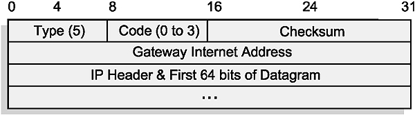
ICMP Destination Unreachable message format
The values relating the code values in the above unreachable message are as follows.

Typical Destination Unreachable code messages
6.6.8 ICMP Query messages
In addition to the reports on errors and exceptional conditions, there is a set of ICMP messages to request information, and to reply to such requests.
Echo Request and Reply
An Echo Request message is sent to the destination node to essentially enquire: ‘Are you alive?’ A reply indicates that the pathway (i.e. the network links in-between as well as the routers) and the destination node are all operating correctly. The structure of the Request and Reply is indicated below.

ICMP Echo Request and Reply format
The first three fields have already been discussed. The additional fields are:
- Type
8 for an Echo Request, and 0 for a Reply - Identifier
A 16-bit random number, used to match a reply message with its associated request message - Sequence number
Used to identify each individual request or reply in a sequence of associated requests or replies with the same source and destination - Data
Generated by the sender and echoed back by the echoer. This field is variable in length; its length and contents are set by the echo request sender. It usually consists of the ASCII characters a, b, c, d, etc
Time-stamp Request and Reply
This can be used to synchronize the clock of a host with that of a time server.

Structure of the Time Stamp Request and Reply
- Type
13 for time-stamp request and 14 for time-stamp reply message - Originate time-stamp
Generated by sender and contains a time value identifying the time the initial time-stamp request was sent - Receive time-stamp
Generated by the echoer and contains the time the original time-stamp was received - Transmit time-stamp
Generated by the echoer and contains a value identifying the time the time-stamp reply message was sent.
The ICMP Time-stamp Request and Reply messages enable a client to adjust its clock against that of an accurate server. The times referred to hereunder are 32-bit integers, measured in milliseconds since midnight, Universal Co-ordinated Time (UCT). This was previously known as Greenwich Mean Time or GMT.
The adjustment is initiated by the client inserting its current time in the ‘originate’ field, and sending the ICMP datagram off to the server. The server, upon receiving the message, then inserts the ‘received’ time in the appropriate field.
The server then inserts its current time in the ‘transmit’ field and returns the message. In practice, the ‘received’ and ‘transmit’ fields for the server are set to the same value.
The client, upon receiving the message back, records the ‘present’ time (albeit not within the header structure). It then deducts the ‘originate’ time from the ‘present’ time. Assuming negligible delays at the server, this is the time that the datagram took to travel to the server and back, or the Round Trip Time (RTT). The time to the server is then one-half of this value.
The correct time at the moment of originating the message at the client is now calculated by subtracting the RTT from the ‘transmit’ time-stamp created by the server. The client calculates its error by the relationship between the ‘originate’ time-stamp and the actual time, and adjust its clock accordingly. By repeated application of this procedure all hosts on a LAN can maintain their clocks to within less than a millisecond of each other.
6.7 Routing protocols
6.7.1 Routing basics
Unlike the Host-to-host layer protocols (e.g. TCP), which control end-to-end communications, IP is rather ‘short-sighted’. Any given IP node (host or router) is only concerned with routing the datagram to the next node, where the process is repeated. Very few routers have knowledge about the entire internetwork, and often the datagrams are forwarded based on default information without any knowledge of where the destination actually is.
Before discussing the individual routing protocols in any depth, the basic concepts of IP routing have to be clarified. This section will discuss the concepts and protocols involved in routing, while the routers themselves will be discussed in Chapter 10.
6.7.2 Direct vs indirect delivery
Refer to Figure 6.39. When the source host prepares to send a message to the destination host, a fundamental decision has to be made, namely: is the destination host also resident on the local network or not? If the NetID portions of the IP address match, the source host will assume that the destination host is resident on the same network, and will attempt to forward it locally. This is called direct delivery.
If not, the message will be forwarded to the ‘default gateway’, i.e. the IP address of a router on the local network. If the router can deliver it directly i.e. the host resides on a network directly connected to the router, it will. If not, it will consult its routing tables and forward it to the next appropriate router.
This process will repeat itself until the packet is delivered to its final destination, and is referred to as indirect delivery.
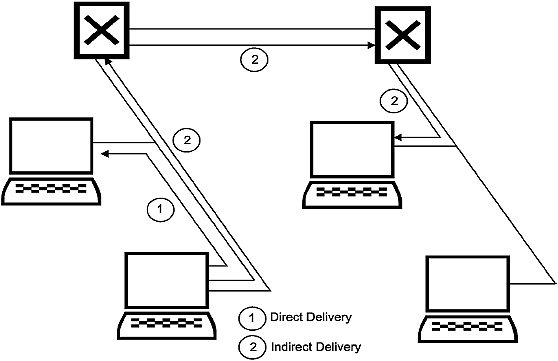
Direct vs indirect delivery
6.7.3 Static versus dynamic routing
Each router has a routing table that indicates the next IP address where the packet has to be sent in order to eventually arrive at its ultimate destination. These routing tables can be maintained in two ways. In most cases, the routing protocols will do this automatically. The routing protocols are implemented in software that runs on the routers, enabling them to communicate with each other on a regular basis, allowing them to share their knowledge of the network with each other. In this way they continuously ‘learn’ about the topology of the system, and upgrade their routing tables accordingly. This process is called dynamic routing.
If, for example, a particular router is removed from the system, the routing tables of all routers containing a reference to that router will change. However, because of the interdependence of the routing tables, a change in any given table will initiate a change in many other routers and it will be a while before the tables stabilize. This process is known as convergence.
Dynamic routing can be further sub-classified as distance vector, link-state or hybrid; depending on the method by which the routers calculate the optimum path.
In distance vector dynamic routing, the ‘metric’ or yardstick used for calculating the optimum routes is simply based on distance, i.e. which route results in the least number of ‘hops’ to the destination. Each router constructs a table that indicates the number of hops to each known network. It then periodically passes copies of its tables to its immediate neighbors. Each recipient of the message simply adjusts its own tables based on the information received from its neighbor.
The major problem with the distance vector algorithm is that it takes some time to converge to a new understanding of the network. The bandwidth and traffic requirements of this algorithm can also affect the performance of the network. Its major advantage is that it is simple to configure and maintain as it only uses the distance to calculate the optimum route.
Link state routing protocols are also known as ‘shortest path first’ protocols. This is based on the routers exchanging link state advertisements to the other routers. Link state advertisement messages contain information about error rates and traffic densities and are triggered by events rather than running periodically as with the distance routing algorithms.
Hybridized routing protocols use both the methods described above and are more accurate than the conventional distance vector protocols. They converge more rapidly to an understanding of the network than distance vector protocols and avoid the overheads of the link state updates. The best example of this one is the Enhanced Interior Gateway Routing Protocol (EIGRP).
It is also possible for a network administrator to make static entries into routing tables. These entries will not change, even if a router that they point to is not operational.
6.7.4 Autonomous Systems
For the purpose of routing, a TCP/IP-based internetwork can be divided into several Autonomous Systems (ASs) or domains. An AS consists of hosts, routers and data links that form several physical networks but is administered by a single authority such as a service provider, university, corporation, or government agency.
ASs can be classified under one of three categories:
- Stub AS
This is an AS that has only one connection to the ‘outside world’ and therefore does not carry any third-party traffic. This is typical of a smaller corporate network - Multi-homed non-transit AS
This is an AS that has two or more connections to the ‘outside world’ but is not setup to carry any third party traffic. This is typical of a larger corporate network - Transit AS
This is an AS with two or more connections to the outside world, and is set up to carry third party traffic. This is typical of an ISP network
Routing decisions that are made within an AS are totally under the control of the administering organization. Any routing protocol, using any type of routing algorithm, can be used within an AS since the routing between two hosts in the system is completely isolated from any routing that occurs in other ASs. Only if a host within one AS communicates with a host outside the AS, will another AS (or ASs) be involved.
6.7.5 Interior and Exterior Gateway Protocols
There are two main categories of TCP/IP routing protocols, namely Interior Gateway Protocols (IGPs) and Exterior Gateway Protocols (EGPs).
Two routers that communicate directly with one another and are both part of the same AS are said to be interior neighbors and are called Interior Gateways. They communicate with each other using IGPs.

Application of routing protocols
In a simple AS consisting of only a few physical networks, the routing function provided by IP may be sufficient. In larger ASs, however, sophisticated routers using adaptive routing algorithms may be needed. These routers will communicate with each other using IGPs such as RIP or OSPF.
Routers in different ASs, however, cannot use IGPs for communication for more than one reason. Firstly, IGPs are not optimized for long-distance path determination. Secondly, the owners of ASs (particularly ISPs) would find it unacceptable for their routing metrics (which include sensitive information such as error rates and network traffic) to be visible to their competitors. For this reason routers that communicate with each other and are resident in different ASs communicate with each other using Exterior Gateway Protocols or EGPs. The Border routers on the periphery, connected to other ASs, must be capable of handling both the appropriate IGPs and EGPs.
The most common EGP (in fact, the only) currently used in the TCP/IP environment is Cisco’s Border Gateway Protocol (BGP), the current version being BGPv4.
6.8 IGPs
The protocols that will be discussed are RIP (Routing Information Protocol), EIGRP (Enhanced Interior Gateway Routing Protocol), and OSPF (Open Shortest Path First).
RIP
RIP originally saw the light as RIP (RFC 1058, 1388) and is one of the oldest routing protocols. The original RIP had a shortcoming in that it could not handle variable-length subnet masks, and hence could not support CIDR. This capability was included with RIPv2. Other versions of RIP include RIPv3 for UNIX platforms and RIPng for IPv6.
RIP is a distance vector routing protocol that uses hop counts as a metric (i.e. form of measurement). Each router, using a special packet to collect and share information about distances, keeps a routing table of its perspective of the network showing the number of hops required to reach each network. In order to maintain their individual perspective of the network, routers periodically pass copies of their routing tables to their immediate neighbors. Each recipient adds a distance vector to the table and forwards the table to its immediate neighbors. The hop count is incremented by one every time the packet passes through a router. RIP only records one route per destination (even if there are more).
Figure 6.41 shows a sample network and the relevant routing tables.
The RIP routers have fixed update intervals and each router broadcasts its entire routing table to other routers at 30-second intervals (60 seconds for Netware RIP). Each router takes the routing information from its neighbor, adds or subtracts one hop to the various routes to account for itself, and then broadcasts its updated table.
Every time a router entry is updated, the timeout value for the entry is reset. If an entry has not been updated within 180 seconds it is assumed suspect and the hop field set to 16 to mark the route as unreachable and it is later removed from the routing table.
One of the major problems with distance vector protocols like RIP is the ‘convergence time’, which is the time it takes for the routing information on all routers to settle in response to some change to the network. For a large network the convergence time can be long and there is a greater chance of frames being misrouted.

RIP tables
RIPv2 (RFC1723) also supports:
- Authentication
This prevents a routing table from being corrupted with incorrect data from a bad source - Subnet masks
The IP address and its subnet mask enable the RIPv2 to identify the type of destination that the route leads to. This enables it to discern the network subnet from the host address - IP identification
This makes RIPv2 more effective than RIP as it prevents unnecessary hops. This is useful where multiple routing protocols are used simultaneously and some routes may never be identified. The IP address of the next hop router would be passed to neighboring routers via routing table updates. These routers would then force datagrams to use a specific route whether or not that route had been calculated to be the optimum route or not using least hop count - Multicasting of RIPv2 messages
This is a method of simultaneously advertising routing data to multiple RIP or RIPv2 devices. This is useful when multiple destinations must receive identical information
RIPng has features similar to that of RIPv2, although it does not support authentication as it uses the standard IPSec security features defined for IPv6.
EIGRP
EIGRP is an enhancement of the original IGRP, a proprietary routing protocol developed by Cisco Systems for use on the Internet. IGRP is outdated since it cannot handle CIDR and VLSM.
EIGRP is a distance vector routing protocol that uses a composite metric for route calculations. It allows for multipath routing, load balancing across 2, 3 or 4 links, and automatic recovery from a failed link. Since it does not only take hop count into consideration, it has better real-time appreciation of the link status between routers and is more flexible than RIP. Like RIP it broadcasts whole routing table updates, but at 90 second intervals.
Each of the metrics used in the calculation of the distance vectors has a weighting factor. The metrics used in the calculation are as follows:
- Hop count. Unlike RIP, EIGRP does not stop at 16 hops and can operate up to a maximum of 255
- Packet size (MTU)
- Link bandwidth
- Delay
- Loading
- Reliability
The metric used is:
Metric = K1 * bandwidth + (K2 * bandwidth)/ (256 – Load) + K3 * Delay
Where K1, K2 and K3 are weighting factors.
Reliability is also added by using the modified metric, which modifies the metric calculated in the first equation above.
Metricmodified = Metric * K5/(reliability + K4)
One of the key design parameters of EIGRP is complete independence from routed protocols. Hence EIGRP has implemented a modular approach to supporting routed protocols and can easily be retrofitted to support any other routed protocol.
OSPF
This was designed specifically as an IP routing protocol, hence it cannot transport any other routing protocols such as IPX. It is encapsulated directly in the IP protocol. OSPF can quickly detect topological changes by flooding link state advertisements to all the other neighbors with reasonably quick convergence.
OSPF is a link state routing or Shortest Path First (SPF) protocol, with the first version detailed in RFC 1131. Version 2 (OSPFv2) was released in 1991 and detailed in RFC 1247. Version 2 was subsequently revised in RFCs 1583, 2178 and 2328 with the last being the current version. With OSPF, each router periodically uses a broadcast mechanism to transmit information to all other routers, about its own directly connected routers and the status of the data links to them. Based on the information received from all the other routers each router then constructs its own network routing tree using the shortest path algorithm.
These routers continually monitor the status of their links by sending packets to neighboring routers. When the status of a router or link changes this information is broadcast to the other routers, which then update their routing tables. This process is known as flooding and the packets sent are very small representing only the link state changes.
Using cost as the metric OSPF can support a much larger network than RIP, which is limited to 15 routers. A problem area can be in mixed RIP and OSPF environments if routers go from RIP to OSPF and back when hop counts are not incremented correctly.
6.9 EGPs
The first Exterior Gateway Protocol was, in fact called EGP! The current de facto Internet standard for inter-domain (AS) routing is BGPv4.
6.9.1 BGPv4
BGPv4, as detailed in RFC 1771, performs intelligent route selection based on the shortest autonomous system path. In other words, whereas IGPs such as RIP make decisions on the number of routers to a specific destination, BGPv4 bases its decisions on the number of ASs to a specific destination. It is a so-called path vector protocol, and runs over TCP (port 179).
BGP routers in one AS speak BGP to routers in other ASs, where the ‘other’ AS might be that of an ISP, or another company. Companies with an international presence and a large, global WAN may also opt to have a separate AS on each continent (running OSPF internally) and run BGP between them in order to create a clean separation.
GGP comes in two ‘flavors’ namely ‘internal’ BGP (iBGP) and ‘external BGP’ (eBGP). IBGP is used within an AS and eBGP between ASs. In order to ascertain which one is used between two adjacent routers, one should look at the AS number for each router. BGP uses a formally registered AS number for entities that will advertise their presence in the Internet. Therefore, if two routers share the same AS number, they are probably using iBGP and if they differ, the routers speak eBGP. Incidentally, BGP routers are referred to as ‘BGP speakers’, all BGP routers are ‘peers’, and two adjacent BGP speakers are ‘neighbors.’
The range of non-registered (i.e. private) AS numbers is 64512–65535 and ISP typically issues these to stub ASs i.e. those that do not carry third-party traffic.
As mentioned earlier, iBGP is the form of BGP that exchanges BGP updates within an AS. Before information is exchanged with an external AS, iBGP ensures that networks within the AS are reachable. This is done by a combination of ‘peering’ between BGP routers within the AS and by distributing BGP routing information to IGPs that run within the AS, such as EIGRP, IS-IS, RIP or OSPF. Note that, within the AS, BGP peers do not have to be directly connected as long as there is an IGP running between them. The routing information exchanged consists of a series of AS numbers that describe the full path to the destination network. This information is used by BGP to construct a loop-free map of the network.
In contrast with iBGP, eBGP handles traffic between routers located on different ASs. It can do load balancing in the case of multiple paths between two routers. It also has a synchronization function that, if enabled, will prevent a BGP router from forwarding remote traffic to a transit AS before it has been established that all internal non-BGP routers within that AS are aware of the correct routing information. This is to ensure that packets are not dropped in transit through the AS.
Objectives
When you have completed this chapter you should be able to:
- Explain the basic functions of the Host-to-Host layer
- Explain the basic operation of TCP and UDP
- Explain the fundamental differences between TCP and UDP
- Decide which protocol (TCP or UDP) to use for a particular application
- Explain the meaning of each field in the TCP and UDP headers
The Host-to-Host communications layer (also referred to as the ‘Service’ layer, or as the ‘Transport’ layer in terms of the OSI model) is primarily responsible for ensuring end-to-end delivery of packets transmitted by IP. This additional reliability is needed to compensate for the lack of reliability in IP.
There are only two relevant protocols residing in this layer, namely TCP (Transmission Control Protocol) and UDP (User Datagram Protocol). In addition to this, the Host-to-host layer includes the APIs (application programming interfaces) used by programmers to gain access to these protocols.
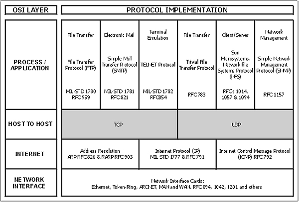
TCP and UDP within the ARPA model
7.1 TCP
7.1.1 Basic functions
TCP is a connection-oriented protocol and is therefore reliable, although this word is used in a data communications context and not in the everyday sense. TCP establishes a connection between two hosts before any data is transmitted. Because a connection is set up beforehand, it is possible to verify that all packets are received on the other end and to arrange re-transmission in the case of lost packets. Because of all these built-in functions, TCP involves significant additional overhead in terms of processing time and header size.
TCP includes the following functions:
- Segmentation of data streams into segments that can be accommodated by IP. The word ‘segmentation’ is used here to differentiate it from the ‘fragmentation’ performed by IP
- Data stream reconstruction from packets received
- Receipt acknowledgment
- Socket services for providing multiple connections to ports on remote hosts
- Packet verification and error control
- Flow control
- Packet sequencing and reordering
In order to achieve its intended goals, TCP makes use of ports and sockets, connection oriented communication, sliding windows, and sequence numbers/acknowledgments.
7.1.2 Ports
Whereas IP can route the message to a particular machine on the basis of its IP address, TCP has to know for which process (i.e. software program) on that particular machine it is destined. This is done by means of port numbers ranging from 1 to 65,535.
Port numbers are controlled by ICANN, the Internet Corporation for Assigned Names and Numbers. This task has previously been handled by its predecessor, IANA, the Internet Assigned Numbers Authority. These numbers can be divided into three groups.
- Well-known ports range from 1 to 1023 and are used, in most cases, for programs that can only be started by privileged users. This means they are typically assigned to servers. HTTP, for example, uses port 80 on the server side.
- Registered port numbers are used where programs can generally be started by normal users, as is the case with clients. These numbers range from 1024 to 49 151, the latter being 75% of 65 536.
- A third group of port numbers is known as Dynamic or Private ports and are also sometimes referred to as ‘ephemeral’ ports. These range from 49,152 to 65 535.
7.1.3 Sockets
In order to identify both the location and application to which a particular packet is to be sent, the IP address (location) and port number (process) is combined into a functional address called a socket. The IP address is contained in the IP header and the port number is contained in the TCP or UDP header.
In order for any data to be transferred under TCP, a socket must exist both at the source and at the destination. TCP is also capable of creating multiple sockets for the same port.
7.1.4 Sequence Numbers
A fundamental notion in the TCP design is that every byte of data sent over the TCP connection has a unique 32-bit number. Of course this number cannot be sent along with every byte, yet it is nevertheless implied. However, the number of the first byte in each segment is included in the accompanying TCP header as a ‘Sequence Number’, and for each subsequent byte that number is simply incremented by the receiver in order to keep track of the bytes.
Before any data transmission takes place, both sender and receiver (e.g. client and server) have to agree on the Initial Sequence Numbers (ISNs) to be used. This process is described under ‘establishing a connection’. Since TCP supports bi-directional operation, both client and server will decide on their individual ISNs for the connection, even though data may only flow in one direction for that specific connection.
The sequence number cannot start at zero every time, as it will create serious problems in the case of short-lived multiple sequential connections between two machines. A packet with a Sequence Number from an earlier connection could easily arrive late, during a subsequent connection. The receiver would have difficulty in deciding whether the packet belongs to a former or to the current connection. It is easy to visualize a similar problem in real life. Imagine tracking a parcel carried by UPS if all agents started issuing tracking numbers beginning with zero every morning.
The Sequence Number is generated by means of a 32-bit software counter that starts at 0 during boot-up and increments at a rate of about once every 4 microseconds (although this varies depending on the operating system being used). When TCP establishes a connection, the value of the counter is read and used as the proposed ISN. This creates an apparently random choice of the ISN.
At some point during a connection the counter could roll over from (232 – 1) and start counting from 0 again. The TCP software takes care of this.
7.1.5 Acknowledgment Numbers
TCP acknowledges data received on a per segment basis, although several consecutive segments may be acknowledged at the same time. Since TCP chooses the segment size in such a way that it fits into the data field of the Data Link layer protocol, each segment is associated with a different frame.
The Acknowledgment Number returned to the sender to indicate successful delivery equals the number of the last byte received plus 1; hence it points to the next expected sequence number. For example: 10 bytes are sent, with Sequence Number equal to 33. This means that the first byte is numbered 33 and the last byte is numbered 42. If received successfully, an Acknowledgment Number of 43 will be returned. The sender now knows that the data has been received properly, as it agrees with that number.
The original version of TCP does not issue selective acknowledgments; so if a specific segment contains errors, the Acknowledgement Number returned to the sender will point to the first byte in the defective segment. This implies that the segment starting with that Sequence Number, and all subsequent segments (even though they may have been transmitted successfully) have to be retransmitted. This creates significant problems for long-delay (satellite) transmissions and in this regard a Selective Acknowledgement (SACK) option has been proposed in RFC 2018.
From the previous paragraph it should be clear that a duplicate acknowledgement received by the sender means that there was an error in the transmission of one or more bytes following that particular Sequence Number.
The Sequence Number and the Acknowledgment Number in a specific header are not related at all. The Sequence Number relates to outgoing data; the Acknowledgement Number refers to incoming data. During the connection establishment phase the Sequence Numbers for both hosts are set up independently; hence these two numbers will never bear any resemblance to each other.
7.1.6 Sliding Windows
Obviously there is a need to get some sort of acknowledgment back to ensure that there is a guaranteed delivery. This technique, called positive acknowledgment with retransmission, requires the receiver to send back an acknowledgment message within a given time. The transmitter starts a timer so that if no response is received from the destination node within a given time, another copy of the message will be transmitted. An example of this situation is given in Figure 7.2.

Positive acknowledgment philosophy
The sliding window form of positive acknowledgment is used by TCP, as it is very time consuming waiting for individual acknowledgments to be returned for each packet transmitted. Hence the idea is that a number of packets (with cumulative number of bytes not exceeding the window size) are transmitted before the source may receive an acknowledgment to the first message (due to time delays, etc). As long as acknowledgments are received, the window slides along and the next packet is transmitted.
During the TCP connection phase each host will inform the other side of its permissible window size. The Window size typically defaults to between 8192 and 32767 bytes. The number is contained in the registry and can be altered manually or by means of ‘tweaking’ software. For example, a Window size of 8192 bytes means that, using Ethernet, five full data frames comprising 5 × 1460 = 7300 bytes can be sent without acknowledgment. At this stage the Window size has shrunk to less than 1000 bytes, which means that unless an ACK is generated, the sender will have to suspend its transmission or send a smaller packet.
The Window field in the TCP header is 16 bits long, giving a maximum window size of 65535 bytes. This is insufficient for satellite links and a solution to this problem will be discussed in chapter 18.
7.1.7 Establishing a connection
A three-way SYN/ SYN_ACK/ACK handshake (as indicated in Figure 7.3) is used to establish a TCP connection. As this is a full duplex protocol it is possible (and necessary) for a connection to be established in both directions at the same time.

TCP connection establishment
As mentioned before, TCP generates pseudo-random sequence numbers by means of a 32-bit software counter. The host establishing the connection reads a value ‘x’ from the counter where x can vary between 0 and (232 –1) and inserts it in the Sequence Number field. It then sets the SYN flag to ‘1’ and transmits the header (no data yet) to the appropriate IP address and port number. Assuming that the chosen sequence number was 132, this action would then be abbreviated as SYN 132.
The receiving host (e.g. the server) acknowledges this by incrementing the received Sequence Number by one, and sending it back to the originator as an Acknowledgment Number. It also sets the ACK flag to ‘1’ in order to indicate that this is an acknowledgment. This results in an ACK 133. The first byte sent by the client would therefore be numbered 133. Before acknowledging, the server obtains its own Sequence Number (y), inserts it in the header, and sets the SYN flag in order to establish a connection in the opposite direction. The header is then sent off to the originator (the client), conveying this message e.g. SYN 567. The composite ‘message’ contained within the header would thus be ACK 133, SYN 567.
The client, upon receiving this, notes that its own request for a connection has been complied with, and also proceeds to acknowledge the server’s request with an ACK 568. Two-way communication is now established.
7.1.8 Closing a connection
An existing connection can be terminated in several ways.
One of the hosts can request to close the connection by setting the FIN flag. The other host can acknowledge this with an ACK, but does not have to close immediately as it may need to transmit more data. This is known as a half-close. When the second host is also ready to close, it will send a FIN that is acknowledged with an ACK. The resulting situation is known as a full close.
Alternatively, either of the nodes can terminate its connection with the issue of RST. However, RST is generally used when either node suspects a faulty connection, for example when it receives a frame with a Sequence Number that clearly does not belong to the current connection.
Both situations are depicted in Figure 7.4.

Closing a connection
7.1.9 The Push operation
TCP normally breaks the data stream into what it regards are appropriately sized segments, based on some definition of efficiency. However, this may not be swift enough for an interactive keyboard application. Hence the Push instruction (PSH bit in the flag field) used by the application program forces delivery of bytes currently in the stream and the data will be immediately delivered to the process at the receiving end.
7.1.10 Maximum Segment Size (MSS)
Both the transmitting and receiving nodes need to agree on the maximum size segments they will transfer. This is specified in the options field.
On the one hand TCP ‘prefers’ IP not to perform any fragmentation as this leads to a reduction in transmission speed due to the fragmentation process, and a higher probability of loss of a packet and the resultant retransmission of the entire packet.
On the other hand, there is an improvement in overall efficiency if the data packets are not too small and a maximum segment size is selected that fills the physical packets that are transmitted across the network. The current specification recommends a maximum segment size of 536 (this is the 576 byte default size of an X.25 frame minus 20 bytes each for the IP and TCP headers). If the size is not correctly specified, for example too small, the framing bytes (headers etc) consume most of the packet size resulting in considerable overhead. Refer to RFC 879 for a detailed discussion on this issue.
Generally speaking, the MSS is always 40 bytes less than the Maximum Transmission Unit (MTU) specified for a link, the difference being the combined size of the default-size IP and TCP headers.
7.1.11 The TCP frame
The TCP frame consists of a header plus data and is structured as follows:

TCP frame format
The various fields within the header are as follows:
Source Port: 16 bits
The source port number.
Destination Port: 16 bits
The destination port number.
Sequence Number: 32 bits
The number of the first data byte in the current segment, except when the SYN flag is set. If the SYN flag is set, a connection is still being established and the sequence number in the header is the initial sequence number (ISN). The first data byte to be sent will then be numbered ISN+1.
Refer to the discussion on Sequence Numbers.
Acknowledgment Number: 32 bits
If the ACK flag is set, this field contains the value of the next sequence number the sender of this message is expecting to receive. Once a connection has been established this is always sent.
Refer to the discussion on Acknowledgment Numbers.
Data Offset: 4 bits
The number of 32- bit words in the TCP header. (Similar to IHL in the IP header.) This indicates where the data begins. The size of the TCP header (even if it includes options) is always a multiple of 32 bits.
Reserved: 6 bits
Reserved for future use. Must be zero.
Control bits (flags): 6 bits
(From left to right)
- URG: Urgent pointer field significant
- ACK: Acknowledgment field significant
- PSH: Push function
- RST: Reset the connection
- SYN: Synchronize sequence numbers
- FIN: No more data from sender
Checksum: 16 bits
The checksum field is the 16-bit one’s complement of the one’s complement sum of all 16-bit words in the header and data. If a segment contains an odd number of header and data bytes to be check-summed, the last byte is padded on the right with zeros to form a 16-bit word for checksum purposes. The pad is not transmitted as part of the segment. While computing the checksum, the checksum field itself is replaced with zeros. This is known as the ‘standard Internet checksum’, and is the same as the one used for the IP header.
The checksum also covers a 96-bit ‘pseudo header’ conceptually appended to the TCP header. This pseudo header contains the source IP address, the destination IP address, the protocol number for TCP (0x06), and the TCP PDU length. This pseudo header is only used for computational purposes and is NOT transmitted. This gives TCP protection against misrouted segments.

Pseudo TCP header format
Window: 16 bits
The number of data bytes, beginning with the one indicated in the acknowledgement field, that the sender of this segment is willing or able to accept.
Refer to the discussion on Sliding Windows.
Urgent Pointer: 16 bits
Urgent data is placed in the beginning of a frame, and the urgent pointer points at the last byte of urgent data (relative to the sequence number i.e. the number of the first byte in the frame). This field is only being interpreted in segments with the URG control bit set.
Options: variable length
Options may occupy space at the end of the TCP header and are a multiple of 8 bits in length. All options are included in the checksum.
7.2 UDP
7.2.1 Basic functions
The second protocol that occupies the Host-to-Host layer is UDP. As in the case of TCP, it makes use of the underlying IP to deliver its PDUs.
UDP is a connectionless or non-connection-oriented protocol and does not require a connection to be established between two machines prior to data transmission. It is therefore said to be an ‘unreliable’ protocol – the word ‘unreliable’ used here as opposed to ‘reliable’ in the case of TCP.
As in the case of TCP, packets are still delivered to sockets or ports. However, since no connection is established beforehand, UDP cannot guarantee that packets are retransmitted if faulty, received in the correct sequence, or even received at all. In view of this one might doubt the desirability of such an unreliable protocol. There are, however, some good reasons for its existence.
Sending a UDP datagram involves very little overhead in that there are no synchronization parameters, no priority options, no sequence numbers, no retransmit timers, no delayed acknowledgement timers, and no retransmission of packets. The header is small; the protocol is fast and streamlined functionally. The only major drawback is that delivery is not guaranteed. UDP is therefore used for communications that involve broadcasts, for general network announcements, or for real-time data. A particularly good application is with streaming video and streaming audio where low transmission overheads are a prerequisite, and where retransmission of lost packets is not only unnecessary but also definitely undesirable.
7.2.2 The UDP frame
The format of the UDP frame as well as the interpretation of its fields are described RFC 768. The frame consists of a header plus data and contains the following fields:
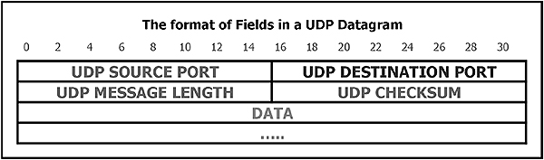
UDP frame format
Source Port: 16 bits
This is an optional field. When used, it indicates the port of the sending process, and may be assumed to be the port to which a reply should be addressed in the absence of any other information. If not used, a value of zero is inserted.
Destination Port: 16 bits
As for source port
Message Length: 16 bits
This is the length, in bytes, of the datagram and includes the header as well as the data. (This means that the minimum value of the length is eight.)
Checksum: 16 bits
This is the 16-bit one’s complement of the one’s complement sum of all the bytes in the UDP Pseudo Header, the UDP header and the data, all strung together sequentially. The bytes are added together in chunks of two bytes at a time and, if necessary, padding in the form of ‘0’s are added to the end to make the whole string a multiple of two bytes.
The Pseudo Header is used for checksum generation only and contains the source IP address from the IP header, the destination IP address from the IP header, the protocol number from the IP header, and the Length from the UDP header. As in the case of TCP, this header is used for computational purposes only, and discarded after the computation. This information gives protection against misrouted datagrams. This checksum procedure is the same as is used in TCP.

UDP pseudo header format
If the computed checksum is zero, it is transmitted as all ‘1’s (the equivalent of ‘0’ in one’s complement arithmetic). An all-zero transmitted checksum value means that the transmitter generated no checksum. This is done for debugging or for higher level protocols that do not care.
UDP is designated protocol number 0x17 (23 decimal or 00010001 binary- see PROTO field in the UDP pseudo header) when used in conjunction with IP.
Objectives
When you have completed study of this chapter you should have a basic understanding of the application and operation of the following application layer protocols:
- FTP
- TFTP
- TELNET
- DNS
- WINS
- SNMP
- SMTP
- POP3
- BOOTP
- DHCP
8.1 Introduction
This chapter examines the uppermost (Application) layer of the TCP/IP stack. Protocols at this layer act as intermediaries between user applications such as clients or servers (external to the stack) and the Host-to-Host layer protocols such as TCP or UDP. An example is HTTP, which acts as an interface between a web server (e.g. Apache) or a web client (e.g. IE6) and TCP.
The list of protocols supplied here is by no means complete, as new protocols are developed all the time. Using a developer’s toolkit such as WinSock, software developers can interface their own Application layer protocols to the TCP/IP protocol stack.
8.2 FTP
FTP (File Transfer Protocol) is specified in RFC 765. File transfer requires a reliable transport mechanism, and therefore TCP connections are used. The FTP process running making the file transfer request is called the FTP client, while the FTP process receiving the request is called the FTP server.
The process involved in requesting a file is as follows:
- The FTP client opens a TCP connection to the control port (21) of the server
- The FTP client forwards a user name and password to the FTP server for authentication. The server indicates whether authentication was successful
- The FTP client sends commands indicating the file name, data type, file type, transmission mode and direction of data flow (i.e. to or from the server) to the server. The server indicates whether the transfer options are acceptable
- The server establishes another TCP connection for data flow, using port 20 on the server
- Data packages are now transferred using the standard TCP flow control, error checking, and retransmission procedures. Data is transferred using the basic Network Virtual Terminal (NVT) format as defined by TELNET. No option negotiation is provided for
- When the file has been transferred, the server closes the data connection, but retains the control connection
The control connection can now be used for another data transfer, or it can be closed
8.2.1 Internal FTP commands
These commands are exchanged between the FTP client and FTP server. Each internal protocol command comprises a four-character ASCII sequence terminated by a new-line (<CRLF>) character. Some commands also require parameters. The use of ASCII character sequences for commands allows the user to observe and understand the command flow, and aids the debugging process. The user can communicate directly with the server program by using these codes, but in general it is much easier to use dedicated client software (e.g. CuteFTP) for this purpose.
FTP commands can be divided into three categories namely service commands, transfer parameter commands and access control commands. There is also a series of reply codes. Here follows a brief summary of the commands and reply codes.
Service commands
These commands define the operation required by the requester. The format of the pathname depends on the specific FTP server being used.
| RETR<SP><pathname><CRLF> | Retrieve a copy of the file from the server |
| STOR<SP><pathname><CRLF> | Store data at the server |
| STOU<CRLF> | Store unique |
| APPE<SP><pathname><CRLF> | Append |
| ALLO<SP><decimal integer> | |
| [<SP>R<SP><decimal integer>]<CRLF> | Allocate storage |
| REST<SP><marker><SP> | Restart transfer at checkpoint |
| RNFR<SP><pathname><CRLF> | Rename from |
| RNTO<SP><pathname><CRLF> | Rename to |
| ABOR<CRLF> | Abort previous service command |
| DELE<SP><pathname><CRLF> | Delete file at server |
| RMD<SP><pathname><CRLF> | Remove directory |
| MKD<SP><pathname><CRLF> | Make directory |
| PWD<CRLF> | Print working directory |
| LIST<SP><pathname><CRLF> | List files or text |
| NLST<SP><pathname><CRLF> | Name list |
| SITE<SP><string><CRLF> | Site parameters |
| SYST<CRLF> | Determine operating system |
| STAT<SP><pathname><CRLF> | Status |
| HELP[<SP><string>]CRLF | Help information |
| NOOP<CRLF> | No operation |
Transfer parameter commands
These commands are used to alter the default parameters used to transfer data on an FTP connection.
| PORT<SP><host-port><CRLF> | Specify the data port to be used. |
| PASV<CRLF> | Request server DTP to listen on a data port |
| TYPE<SP><type code><CRLF> | Representation type: ASCII, EBCDIC, image, or local. |
| STRU<SP><structure code><CRLF> | File structure: file, record or page. |
| MODE<SP><mode code><CRLF> | Transmission mode: stream, block or compressed |
Access control commands
These commands are invoked by the server and determine which users may access a particular file.
| USER<SP><username> <CRLF> | User name |
| PASS<SP><password><CRLF> | User password |
| ACCT<SP><acc. information><CRLF> | User account |
| CWD<SP><pathname><CRLF> | Change working directory |
| CDUP<CRLF> | Change to parent directory |
| SMNT<SP><pathname><CRLF> | Structure mount |
| REIN<CRLF> | Terminate user and re-initialize |
| QUIT<CRLF> | Logout |
| <SP> | Space character |
| <CRLF> | Carriage return, line feed characters |
Reply codes
FTP uses a three-digit return code ‘xyz’ followed by a space to indicate transfer conditions. The first digit (value 1–5) indicates whether a response is good, bad or incomplete. The second and third digits are encoded to provide additional information about the reply. The values for the first digit are:
| Value | Description |
| 1yz | Action initiated. Expect another reply before sending a new command. |
| 2yz | Action completed. Can send a new command. |
| 3yz | Command accepted but on hold due to lack of information. |
| 4yz | Command not accepted or completed. Temporary error condition exists. Command can be reissued. |
| 5yz | Command not accepted or completed. Don’t reissue – reissuing the command will result in the same error. |
The second digit provides more detail about the condition indicated by the first digit:
| Value | Description |
| x0z | Syntax error or illegal command |
| x1z | Reply to request for information |
| x2z | Reply that refers to connection management |
| x3z | Reply for authentication command |
| x5z | Reply for status of server |
The third digit of the reply code also provides further information about the condition, but the meanings vary between implementations.
8.2.2 FTP user commands
Although designed for use by applications, FTP software usually also provides interactive access to the user, with a range of commands that can be used to control the FTP session. There are several dozen commands available to the user, but for normal file transfer purposes very few of them ever need to be used.
| Command | Description |
| ASCII | Switch to ASCII transfer mode |
| binary | Switch to binary transfer mode |
| cd | Change directory on the server |
| cdup | Change remote working directory to parent directory |
| close | Terminate the data connection |
| del | Delete a file on the server |
| dir | Display the server directory |
| get | Get a file from the server |
| help | Display help |
| ls | List contents of remote directory |
| lcd | Change directory on the client |
| mget | Get several files from the server |
| mput | Send several files to the server |
| open | Connect to a server |
| put | Send a file to the server |
| pwd | Display the current server directory |
| quote | Supply a file transfer protocol (FTP) command directly |
| quit | Terminate the file transfer protocol (FTP) session |
| trace | Display protocol codes |
| verbose | Display all information |
To execute a command, the user types the commands at the ftp prompt, e.g.
ftp>close
A list of available user commands can be viewed by typing help at the ftp prompt, e.g.
ftp> help close
After logging into another machine using FTP, the user is still logically connected to the (local) client machine. This is different to TELNET, where the user is logically connected to the (remote) server machine. References to directories and movements of files are therefore relative to the client machine. For example, getting a file involves moving it from the server to the client; putting a file involves moving it from the client to the server.
It may be wise to create a special directory on the client computer just for the transfer of files into and out of the client’s system. This helps guard against accidental file deletion, and allows easier screening of incoming files for viruses.
Most FTP clients have a GUI-based interface that displays the file systems of the local and the remote machines in two separate windows and allows file transfers from one machine to another by mouse movements on the screen.
Most UNIX machines act as FTP servers by default. A daemon process watches the TCP command port (21) continuously for the arrival of a request for a connection and calls the necessary FTP processes when one arrives. Windows does not include FTP server software, but Internet Explorer has a built-in FTP client.
Anonymous FTP access allows a client to access publicly available files using the login name ‘anonymous’ and the password ‘guest’. Alternatively the password may be required to resemble an e-mail address. Public files are often placed in separate directories on FTP servers.
8.3 TFTP
8.3.1 Introduction
Trivial File Transfer Protocol (RFC 1350) is less sophisticated than FTP, and caters for situations where the complexity of FTP and the reliability of TCP is neither desired nor required. TFTP does not log on to the remote machine; so it does not provide user access and file permission controls.
TFTP is used for simple file transfers and typically resides in the ROM of diskless machines such as PLCs that use it for bootstrapping or to load applications.
The absence of authorization controls can be overcome by diligent system administration. For example, on a UNIX system, a file may only be transferred if it is accessible to all users on the remote machine (i.e. both read and write permissions are set).
TFTP does not monitor the progress of the file transfer so does not need the reliable stream transport service of TCP. Instead, it uses UDP, with time-out and retransmission mechanisms to ensure data delivery. The UDP source and destination port fields are used to create the socket at each end, and TFTP Transfer IDentifiers (TIDs) ranging between 0 and 65,535 are created by TFTP and passed to UDP to be placed in the UDP header field as a source port number. The destination (server) port number is the well-known port 69, reserved for TFTP.
Data is relayed in consecutively numbered blocks of 512 bytes. Each block must be acknowledged, using the block number in the message header, before the next block is transmitted. This system is known as a ‘flip-flop’ protocol. A block of less than 512 bytes indicates the end of the file. A block is assumed lost and re-sent if an acknowledgment is not received within a certain time period. The receiving end of the connection also sets a timer and, if the last block to be received was not the end of file block, the receiver will re-send the last acknowledgment message once the time-out has elapsed.
TFTP can fail for many reasons and almost any kind of error encountered during the transfer will cause complete failure of the operation. An error message sent either in place of a block of data or as an acknowledgment terminates the interaction between the client and the server.
8.3.2 Frame types
There are five TFTP package types, distinguished by an operation code (‘opcode’) field. They are:
| Opcode | Operation |
| 1 | Read request (RRQ) |
| 2 | Write request (WRQ) |
| 3 | Data (DATA) |
| 4 | Acknowledgment (ACK) |
| 5 | Error (ERROR) |
The frames for the respective operations are constructed as follows:
RRQ/WRQ frames

RRQ/WRQ frame format
The various fields are as follows:
- Opcode: 2 bytes
1 for RRQ, 2 for WRQ - Filename: variable length
Written in NetASCII, defined in ANSI X3.4-1968. Terminated by a 0 byte. - Mode: variable length
Indicates the type of transfer. Terminated by a 0 byte. The three available modes are:- NetASCII
- Byte – raw 8-bit bytes and binary information
- Mail – indicates destination is a user not a file – information transferred as NetASCII
DATA frames
The file name does not need to be included as the IP address and UDP protocol port number of the client are used as identification.

Data frame format
The fields are as follows:
- Opcode: 2 bytes
3 indicates ‘data’ - Block number: 2 bytes
The particular 512-byte block within a specific transfer (allocated sequentially) - Data: Variable, 1–512 bytes.
Data is transmitted as consecutive 512-byte blocks; a frame with less than 512 bytes means that it is the last block of a particular transfer
ACK frames
These frames are sent to acknowledge each block that arrives. TFTP uses a ‘lock-step’ method of acknowledgment, which requires each data packet to be acknowledged before the next can be sent.

ACK frame format
The fields are as follows:
- Opcode: 2 bytes
4 indicates acknowledgment - Block number: 2 bytes
The number of the block being acknowledged
Error frames
An error message causes termination of the operation.

Error frame
The fields are:
- Opcode: 2 bytes
5 indicates an error - Error code: 2 bytes
This field contains a code that describes the problem- 0 Not defined
- 1 File not found
- 2 Access violation
- 3 Disk full/allocation exceeded
- 4 Illegal operation
- 5 Unknown transfer operation
- 6 File already exists
- 7 No such user
- Error message: Variable length string
This is NetASCII string, terminated by a 0 byte
8.4 TELNET
TELNET (TELecommunications NETwork) is a simple remote terminal protocol that enables virtual terminal capability across a network. That is, a user on machine A can log in to a server on machine B across a network. If the remote machine has a TELNET server installed, user A can log into it and execute keyboard commands on machine B as if he is operating on his own machine.
The procedure for connecting to a remote computer depends on how the user access permissions are set up. The process is generally menu driven. Some remote machines require the user to have an account on the machine and will request a username and password. However, many information resources are available to the user without an account and password. TELNET is also often used to gain access to managed devices such as switches and routers.
TELNET achieves a connection to the remote server via its well-known port number, using either the server’s domain name or its IP address, and then passes keystrokes to the remote server and receives output back from it.
TELNET treats both ends of the connection similarly, so that software at either end of a connection can negotiate the parameters that will control their interaction. It provides a set of options such as type of character set to be used (7-bit or 8-bit), type of carriage-return character to be recognized (e.g. CR or LF) etc, which can be negotiated to suit the client and the server. It is possible for a machine to act as both client and server simultaneously, enabling the user to log into other machines while other users log into his machine.
In the case of a server capable of managing multiple concurrent connections, TELNET will listen for new requests and then create a new instantiation (or ‘slave’) to deal with each new connection.
The TELNET protocol uses the concept of a Network Virtual Terminal (NVT) to define each end of a connection. NVT uses standard 7-bit US ASCII codes to represent printable characters and control codes such as ‘move right one character’, ‘move down one line’, etc. 8-bit bytes with the high order bit set are used for command sequences. Each end has a virtual keyboard that can generate characters (it could represent the user’s keyboard or some other input stream such as a file) and a logical printer that can display characters (usually a terminal screen). The TELNET programs at either end handle the translation from virtual terminal to physical device. As long as this translation is possible, TELNET can interconnect any type of device. When the connection is first established and the virtual terminals are set up, they are provided with codes that indicate which operations the relevant physical devices can support.
An operating system usually reserves certain ASCII keystroke sequences for use as control functions. For example, an application running on UNIX operating systems will not receive the Ctrl-C keystroke sequence as input if it has been reserved for interrupting the currently executing program. TELNET must therefore define such control functions so that they are interpreted correctly at both ends of the connection. In this case, Ctrl-C would be translated into the TELNET IP command code.
TELNET does not use ASCII sequences to represent command codes. Instead, it encodes them using an escape sequence. This uses a reserved byte, called the ‘Interpret As Command’ (IAC) byte, to indicate that the following byte contains a control code. The actual control code can be represented as a decimal number, as follows:
| Command | Decimal Value | Meaning |
|---|---|---|
| EOR | 239 | End of record |
| SE | 240 | End of option sub-negotiation |
| NOP | 241 | No operation |
| DMARK | 242 | Data mark – the data stream part of a SYNCH (always marked by TCP as urgent) |
| BRK | 243 | Break |
| IP | 244 | Interrupt process – interrupts or terminates the active process |
| AO | 245 | Abort output – allows the process to run until completion, but does not send the end of record command |
| AYT | 246 | Are you there – used to check that an application is functioning at the other end |
| EC | 247 | Erases a character in the output stream |
| EL | 248 | Erases a line in the output stream |
| GA | 249 | Go ahead – indicates permission to proceed when using half-duplex (no echo) communications |
| SB | 250 | Start of option sub-negotiation |
| WILL | 251 | Agreement to perform the specified option or confirmation that the specified option is now being performed |
| WON’T | 252 | Refusal to perform the specified option or confirmation that the specified option will no longer be performed |
| DO | 253 | Asks for the other end to perform the specified option, or acknowledges that the other end will perform the specified option |
| DON’T | 254 | Demands that the other end stops performing the specified option, or confirmation that the other end is no longer performing the specified option |
| IAC | 255 | Interpret as command i.e. interpret the next octet as a command. When the IAC octet appears as data, the 2-octet sequence sent will be IAC-IAC |
The IAC character to have the above meanings must precede the control code. For example, the two-octet sequence IAC-IP (or 255-244) would induce the server to abort the currently executing program.
The following command options are used by TELNET:
| Option Code | Meaning |
|---|---|
| 0 | Transmit binary – change transmission to 8-bit binary |
| 1 | Echo |
| 2 | Reconnection |
| 3 | Suppress go ahead – i.e. no longer send go-ahead signal after data |
| 4 | Approximate message size negotiation |
| 5 | Status request – used to obtain the status of a TELNET option from the remote machine. |
| 6 | Request timing mark – used to synchronize the two ends of a connection |
| 7 | Remote controlled transmission and echo |
| 8 | Output line width |
| 9 | Output page length |
| 10 | Output carriage-return action |
| 11 | Output horizontal tab stop setting |
| 12 | Output horizontal tab stop action |
| 13 | Output form feed action |
| 14 | Output vertical tab stop setting |
| 15 | Output vertical tab stop action |
| 16 | Output line feed action |
| 17 | Extend ASCII characters |
| 18 | Logout |
| 24 | Terminal type – used to exchange information about the make and model of a terminal being used |
| 25 | End of record – sent at end of data |
| 28 | Terminal location number |
| 31 | Window size |
| 34 | Line-mode – uses local editing and sends complete lines instead of individual characters. |
The two-byte sequence may be followed by a third byte containing optional parameters.
An optional code of 1 indicates ‘ECHO’; therefore, the three octets sequence 255-251-1 means ‘WILL ECHO’ and instructs the other end to begin echoing back the characters that it receives. A command sequence of 255-252-1 indicates that the sender either will not echo back characters or wants to stop echoing.
The negotiation of options allows clients and servers to optimize their interaction. It is also possible for newer versions of TELNET software that provide more options to work with older versions, as only the options that are recognized by both ends are negotiated.
If the server application malfunctions and stops reading data from the TCP connection, the operating system buffers will fill up until TCP eventually indicates to the client system a window size of zero, thus preventing further data flow from the client. In such a situation TELNET control codes will not be read and therefore will have no effect. To bypass the normal flow control mechanism, TELNET uses an ‘out of band’ signal. Whenever it places a control signal in the data stream, it also sends a SYNCH command and appends a data mark octet. This induces TCP to send a segment with the URGENT DATA flag set, which reaches the server directly and causes it to read and discard all data until it finds the data mark in the data stream, after which it returns to normal processing.
TELNET programs are freely available and can be downloaded via the Internet. Windows 95/98 included a simple Windows-type interface called Microsoft TELNET 1.0 but, in later versions of Windows, Microsoft has reverted to command-line instructions.
The options for the TELNET command line input is as follows:
telnet [-a][-e escape char][-f log file][-l user][-t term][host[port]]
| -a | Attempt automatic logon. Same as –l option except uses the currently logged on user’s name. |
| -e | Escape character to enter telnet client prompt. |
| -f | File name for client side logging. |
| -l | Specifies the user name to log in with on the remote system. Requires that the remote system support the TELNET ENVIRON option |
| -t | Specifies terminal type. Supported term types are vt100, vt52, ansi and vtnt only. |
| host | Specifies the hostname or IP address of the remote computer to connect to. |
| port | Specifies the port number or service name. |
In its simplest form, the TELNET command for connecting to the POP3 server on host 192.168.0.1 would be
C:\>telnet 192.168.0.1 110
8.5 DNS
8.5.1 Name resolution using the Hosts file
On a small TCP/IP network each individual host can (optionally) have a list of names by which it refers to other hosts. These given names can differ from host to host and are not to be confused with the ‘computer name’ (NetBIOS name) entered on each machine. They can be considered nicknames (e.g. ‘Charlie’ instead of ‘192.176.44.56’) and the mapping between these names and their associated IP addresses is maintained as a ‘flat’ database in the Hosts file on each host. The resolver process on each host translates host names into IP addresses by a simple lookup procedure. On Windows XP this file is located at C:\windows\systen32\drivers\etc\hosts. The correct Hosts file has no extension, unlike the sample Hosts file stored as hosts.sam.
In a large network the HOSTS files would have to be identical on all machines. The maintenance of these files to reflect additions and changes can become quite a tedious task. On the Internet, with its millions of names, this becomes impossible.
8.5.2 Name resolution using DNS
The Domain Name System (DNS) provides a network-wide (and in the case of the Internet – a world-wide) directory service that maps host names against IP addresses. For most users this is a transparent process and it is to them irrelevant whether the resolution takes place via a hosts file or via DNS.
When the IP address of a specific destination host has to be resolved, the DNS resolver on the requesting host contacts its designated Local (DNS) Name Server, the IP address of which is contained in the IP configuration of the requesting host. The Local Name Server then, in turn, contacts the Root Domain Name Server (maintained by InterNIC) in order to locate the Primary Name Server that contains the required domain name records. The Root Domain Name Server returns the IP address of the appropriate Primary Name Server to the Local Name Server, which now contacts the appropriate Primary Name Server directly and requests the IP address for the given name. If the Primary Name Server cannot find the name, the request goes to the Secondary Name Server.
The Primary and Secondary name servers maintain a tree-structured directory database. The collective database stored on all the DNS Name Servers forms a global namespace of all the hosts that can be referenced anywhere on the Internet.
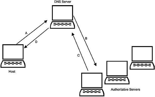
DNS name resolution
The Internet naming scheme hierarchical namespace
The original Internet namespace was ‘flat’ i.e. it had no hierarchical structure. At this stage it was still administered by the Network Information Center (NIC). The task eventually became too large because of the rapidly increasing number of hosts and a hierarchical (tree-structured) namespace was adopted. At present, the ultimate responsibility for the maintenance of this namespace is vested in the ICANN.
In a domain name the most local domain is written first and the most global domain is written last. The domain name purdue.edu might identify Purdue University. This domain name is registered against a specific IP address. The administrator of this domain name may now create sub-domains such as, say, cs.purdue.edu for the computer science department at Purdue University. The administrator of the computer science department, in turn, may assign a Fully Qualified Domain Name (FQDN) to an individual host, such as computer1.cs.purdue.edu.
If a user is referring to a specific host within a local network, a FAQN is not needed, as the DNS resolver will automatically supply the missing high-level domain name qualifier.
The following commands are therefore equivalent when an ftp client and ftp server are located on the same network:
- ftp computer1.purdue.edu
- ftp computer1
Standard domain names
The original namespace contained a set of standard top-level domains without any reference to a specific country. Since the original Internet was not envisaged to exist beyond the borders of the United States, the absence of any reference to a country implies an organization within the USA.
The following are some of the common top-level domains administered by ICANN. More detailed information can be obtained from www.icann.org.
- .com Commercial organizations
- .net Major network support centers
- .edu Educational institutions
- .gov Government institutions (United States government only)
- .mil Military groups (United States military only)
- .int Organizations established by international treaties between governments, or Internet infrastructure databases
- .org Organizations other than the above
Domain names for the .com, .net and .org domains can be obtained from various accredited re-sellers.
Country codes
As the Internet backbone was extended into countries other than the USA, the top-level domain names were extended with a two-letter country code as per ISO 3166 (e.g. uk for the United Kingdom, au for Australia, za for South Africa, ca for Canada). The complete list of all Country Code Top-Level Domains (CCTLDs) can be obtained from the ICANN website. This site also contains the basic information for each CCTLD such as the governing agency, administrative and technical contact names telephone and fax numbers, and server information. This information can also be obtained from the Network Solutions web site.
DNS clients and servers
Each host on a network that uses the DNS system runs the DNS client software, which implements the resolver function. Designated servers, in turn, implement the DNS name server functions. In processing a command that uses a domain name instead of an IP address, the TCP/IP software automatically invokes the DNS resolver function.
On a small network one name server may be sufficient and the name server software may run on a machine already used for other server purposes (such as a Windows 2003 machine acting as a file server). On large networks it is prudent to run at least two Local Name Servers for reasons of availability, viz. a primary and a secondary name server. On large internetworks it is also common to use multiple Primary Name Servers, each of which contains a portion of the namespace. It is also possible to replicate portions of the namespace across several servers in order to increase availability.
A network connected to the Internet needs access to at least one Primary Name Server and one Secondary Name Server, both capable of performing naming operations for the registered domain names on the Internet. In the case of the Internet, the number of domain names is so large that the namespace is distributed across multiple Primary and Secondary servers in different countries. For example, all the co.za domain names are hosted across several name servers located in South Africa.
The DNS client resolver software can implement a caching function by storing the results from the name resolution operation. In this way the resolver can resolve a future query by looking up the cache rather than actually contacting the name server. Cache entries are given a Time To Live so that they are purged from the cache after a given amount of time.
DNS frame format
The message format for DNS messages is as follows.

DNS message format
- ID (IDENTIFICATION), a tracking number (16 bits) used to correlate queries and responses
- QR, a one-bit flag that identifies the message as a query (QR=0) or a
response (QR=1) - OPCODE. This 4-bit field further defines a query as follows:
- 0 = Standard query
- 1= Inverse query
- 2 = Server status request
- The other opcodes (3–15) are not used
- Flags, used to describe the message further. They are, from right to left:
- Authoritative answer (AA)
- Truncation (TC)
- Recursion desired (RD)
- Recursion available (RA)
- RCODE, the last field in the first long-word is used for response codes with the following meanings:
- 0 = No error
- 1 = Format error
- 2 = Server error
- 3 = Name error
- 4 = Not used
- 5 = Refused
- Four COUNT fields indicate the length of the fields to follow:
- QDCOUNT gives the number of question entries
- ANCOUNT gives the number of resource records in the answer section
- NSCOUNT refers to the number of name server resource records in the Authority section
- ARCOUNT refers to the number of resource records in the additional records section
- Question section
Contains queries. A query consists of a query domain name field containing the FQDN about which information is required, a query type field specifying the type of information required, and a query class field identifying the protocol suite with which the name is associated - Answer section
Contains information returned in response to a query. The resource domain name, type, and class fields are from the original query. The Time To Live field specifies how long this information can be used if it is cached at the local host. The format of the resource data field depends on the type of information required - Authority section
Identifies the server that actually provided the information if a name server has to contact another name server for a response. The format for this field is the same as for the answer section - Additional query information
Contains additional information related to the name in query; (e.g. the IP address of the host that is the mail exchanger, in response to a MX query)
The DNS message contains a query type field, since the name server database consists of many types of information. The following list shows some of the types:
- A Host IP address
- CNAME Canonical domain name for an alias
- MINFO Information about a mailbox or mail list
- MX Name of a host that acts as mail exchanger for a domain
- NS Name of authoritative server for a domain
- PTR Domain name
- SOA Multiple fields that specify which parts of the naming hierarchy a server implements
8.6 WINS
8.6.1 Introduction
WINS is not a general TCP/IP Application layer protocol, but rather a Microsoft Windows-specific utility with the primary role of NetBIOS name registration and resolution on TCP/IP. In many respects WINS is like DNS. However, while DNS resolves TCP/IP host names to static IP addresses, WINS resolves NetBIOS names to dynamic addresses assigned by DHCP.
WINS maintains a database on the WINS server. This database provides a computer name to IP address mapping, allowing computers on the network to interconnect on the basis of machine names. It also prevents two machines from registering the same name. With traditional NetBIOS name resolution techniques that rely on broadcast messages, it is not possible to browse across an IP router. WINS overcomes this problem by providing name resolution regardless of host location on the network. Since it reduces the number of the broadcast packets normally used to resolve NetBIOS names, it can also improve the network performance.
WINS uses a client/server model and, in order to run it on a network, at least one WINS server is needed. The WINS server must have a statically assigned IP address, entered into the TCP/IP configuration for all machines on the network that want to take advantage of the WINS server for name resolution and name registration.
WINS is configured on XP client machines by selecting Control Panel ->Network Connections ->Local Area Connection ->Properties ->Internet Protocol (TCP/IP) ->Properties ->Advanced ->WINS.

WINS configuration screen (courtesy Microsoft Corporation)
8.6.2 WINS name registration
When a WINS client is turned on for the first time it tries to register its NetBIOS name and IP address with the WINS server by sending a name registration request via UDP. When the WINS server receives the request it checks its database to ensure the requested NetBIOS name is not in use on the network. If the name registration is successful, the server sends a name registration acknowledgment back to the client. This acknowledgment includes the Time To Live for the name registration. The TTL indicates how long the WINS server will keep the name registration before canceling it. It is the responsibility of the WINS client to send a name refresh request to the WINS server before the name expires, in order to keep the name.
If the client tries to register a name that is already in use, the WINS server sends a denial message back to the client. The client than displays a message informing the user that the computer name is already in use on the network.
When a WINS client shuts down it sends a name release request to the WINS server, releasing its name from the WINS database.
8.6.3 WINS name resolution
When a WINS-enabled client needs to resolve the NetBIOS name to IP address, it uses a resolution method called ‘h-node name resolution’, which includes the following procedures:
- It verifies that the name request doesn’t point to itself
- It looks in its name resolution cache for a match. Names remain in the cache for about 10 minutes
- It then sends a direct name lookup to the WINS server. If the WINS server can match the name to an IP address, it sends a response to the client
- If the WINS server cannot do the match, the client broadcasts to the network
- If there is still no response the client will look into its own local LMHOSTS file
- Finally the client will look into the local HOSTS file, or ask the DNS if it has a matching host name. This is only done if the client is configured to use DNS for NetBIOS name resolution
8.6.4 WINS proxy agents
WINS proxy agents are used to allow non-WINS-enabled clients to interact with a WINS service. A WINS proxy agent listens to the local network for clients trying to use broadcasting to resolve NetBIOS names. The WINS proxy agent picks these requests off the network and forwards them to the WINS server, which responds with the resolved IP address. The WINS proxy agent then provides this information to the client requesting the name resolution.
The advantage of this system is that there is no need to make any changes to the existing non-WINS-enabled clients, and in fact they are completely unaware that the name resolution has been provided by the WINS service.
8.7 SNMP
The Simple Network Management Protocol (SNMP) is an Application layer protocol that facilitates the exchange of management information between network devices. It allows network administrators to manage network performance, find and solve network problems, and plan for network growth.
There are three versions of SNMP namely SNMPv1, SNMPv2 and SNMPv3). They all have a number of features in common, but SNMPv2 includes enhancements such as additional protocol operations, and SNMPv3 adds security and administration.
8.7.1 SNMP basic components
An SNMP managed network consists of three key components namely Managed Devices, Agents and Network Management Systems:
- Managed Devices are network nodes that contain SNMP agents and reside on a managed network. These devices collect and store management information and make this information available to Network Management Systems (NMSs) using SNMP. Managed devices can be routers, access servers, switches, bridges, hubs, computer hosts or printers
- An Agent is a network management software module that resides in a managed device. It has local knowledge of management information and translates that information into a form compatible with SNMP
- NMSs execute applications that monitor and control managed devices. They provide the bulk of the processing and memory resources required for network management. One or more NMSs must exist on any managed network
8.7.2 SNMP basic commands
Managed devices are monitored and controlled using four basic SNMP commands namely read, write, trap, and traversal operations:
- The read command is used by an NMS to monitor managed devices. The NMS examines different variables that are maintained by managed devices
- The write command is used by an NMS to control managed devices. The NMS changes the values of variables stored within managed devices
- The trap command is used by managed devices to asynchronously report the events to the NMS. When certain types of events occur, a managed device sends a trap to the NMS
- Traversal operations are used by the NMS to determine which variables a managed device supports and to sequentially gather information in variable tables, such as a routing table
8.7.3 SNMP MIB
A Management Information Base (MIB) is a collection of information that is organized hierarchically. MIBs are accessed using a network management protocol such as SNMP. They comprise managed objects and are identified by object identifiers.
A managed object (sometimes called a ‘MIB object’, an ‘object’, or a ‘MIB’) is one of any number of specific characteristics of a managed device. Managed objects comprise one or more ‘object instances’, which are essentially variables.
There are two types of managed objects, namely scalar and tabular. Scalar objects define a single object instance. Tabular objects define multiple related object instances that are grouped together in MIB tables. An example of a managed object is ‘at Input’, which is a scalar object containing a single object instance viz. the integer value that indicates the total number of input Novell Netware packets on a router interface. An object identifier (or object ID) uniquely identifies a managed object in the MIB hierarchy. The MIB hierarchy can be depicted as a tree with a nameless root, the levels of which are assigned by different organizations.

MIB tree
The top-level MIB object IDs belong to different standards organizations, while lower-level object IDs are allocated by associated organizations. Vendors can define private branches that include managed objects for their own products. MIBs that have not been standardized are typically positioned in the experimental branch. The managed object at Input can be uniquely identified either by the object name viz. iso.identified-organization. dod.internet.private.enterprise.cisco.temporary_variables.Novell.atInput, or by the equivalent object descriptor 1.3.6.1.4.1.9.3.4.1.
8.7.4 SNMPv2 operation
SNMP is a simple request–response protocol. The network-management system issues a request, and managed devices return responses. This behavior is implemented by using one of four protocol operations viz. Get, GetNext, Set, and Trap.
- The Get operation is used by the NMS to retrieve the value of one or more object instances from an agent. If the agent responding to the Get operation cannot provide values for all the object instances in a list, it does not provide any values
- The GetNext operation is used by the NMS to retrieve the value of the next object instance in a table or list within an agent
- The Set operation is used by the NMS to set the values of object instances within an agent
- The Trap operation is used by agents to asynchronously inform the NMS of a significant event
The Get, GetNext, and Set operations used in SNMPv2 are exactly the same as that used in SNMPv1. SNMPv2, however, adds and enhances some operations. The SNMPv2 Trap operation, for example, serves the same function as that used in SNMPv1. However, it uses a different message format and is designed to replace the SNMPv1 Trap. SNMPv2 also defines two additional protocol operations: GetBulk and Inform:
- The GetBulk operation is used by the NMS to efficiently retrieve large blocks of data, such as multiple rows in a table. It fills a response message with as much of the requested data as will fit
- The Inform operation allows one NMS to send trap information to another NMS and receive a response. In SNMPv2, if the agent responding to GetBulk operations cannot provide values for all the variables in a list, it provides partial results
SNMPv1 and SNMPv2 are, however, not secure, with the result that hackers can easily exploit them to gain unauthorized access to SNMP-enabled devices. These weaknesses have been addressed in SNMPv3, which supports authentication, privacy and access control.
8.8 SMTP
TCP/IP defines an electronic messaging protocol named Simple Mail Transfer Protocol or SMTP. SMTP is used by e-mail clients such as Outlook Express or Eudora to send messages and files to an e-mail server on a remote network, usually that of an ISP.
SMTP defines the interchange between the user’s e-mail client and the ISP’s mail server. It does not define how the mail is to be delivered to the ultimate recipient. Although mail is normally forwarded to an SMTP server by an e-mail client, it is also possible to log directly into the server via TELNET and interact with command-line entries.
The first step in the transmission of the data is the connection setup, whereby the SMTP client opens a TCP connection to the remote SMTP server at port 25. The client then sends an optional ‘Helo’ (sic) command and the SMTP server sends a reply indicating its ability to receive mail. TELNET users will have to enter the IP address or the domain name of the server (e.g. smtp1.attglobal.net), the relevant port number (25) and possibly a terminal type (e.g. VT-100). The first two items are necessary for TCP to create the socket.
The second step in the process involves the actual mail transfer. Mail transfer begins with a ‘Mail From’ command containing the name of the sender, followed by a ‘Receipt’ command indicating the recipient. A ‘Data’ command is followed by the actual message. SMTP can be considered a reliable delivery service in that the underlying TCP protocol ensures correct delivery to the SMTP server. SMTP, however, neither guarantees nor offers mechanisms for reliable delivery from the SMTP server to the recipient.
When the message transfer is complete another message can be sent, the direction of transfer changed, or the connection closed. Closing the connection involves the SMTP client issuing a ‘Quit’ command. Both sides then execute a TCP close operation in order to release the connection.
SMTP commands begin with a four-byte command code (in ASCII), which can be followed by an argument. The SMTP replies use the same format as FTP, i.e. a 3-digit numeric value followed by a text string. Here follows some SMTP commands.
- HELO
- MAIL FROM: sender-e-mail-address
- VRFY recipient-mail-address
- RCPT TO: recipient-e-mail-address
- EXPN alias-name
- DATA
- HELP command-name
- RSET
- NOOP
- QUIT
In the following example a simple ASCII string is sent to a recipient via a TELNET connection. The ‘period’ (full stop), in a separate line, is required to send the message. Some lines have been printed in italics to indicate that they are responses from the server.
220 prserv.net – Maillenium ESMTP/ MULTIBOX out4 #30
MAIL FROM: john@hotmail.com
250 ok
RCPT TO: deb@iinet.net.au
250 ok; forward to <deb@iinet.net.au)
DATA
354 ok
‘This is only a test message.’
.
250 ok, id = 2000042800030723903cb80fe
QUIT
8.9 POP
The current version of the Post Office Protocol is POP3. POP3 uses the well-known port 110. Like SMTP, it involves a client running on a local machine and a server running on a remote machine. POP3 is very much the opposite of SMTP in that its function is to retrieve mail from a remote POP3 server to a local POP3 client.
It was developed to ease the load on mail servers. Instead of multiple clients logging in for long periods to a remote mail server (as is the case, for example, with Hotmail) the POP3 client makes a quick connection to the mail server, retrieves the mail (optionally deleting it from the server), then breaks the connection. As in the case of SMTP, it uses a TCP connection for this purpose. Unlike SMTP, proper authentication with a user name and a password is required.
POP3 commands include the following.
- STAT
- LIST message-number
- RETR message-number
- DELE message-number
- NOOP
- RSET
- QUIT
- TOP message-number number-of-lines
The following example shows the interaction with a POP3 server via a
TELNET connection. Server responses are printed in italics.
+OK POP Server Version 1.0 at pop1a.prserv.net
USER auinet.deb
+OK Password required for deb
PASS geronimo
+OK deb has 2 messages (750 octets)_
LIST
+OK 2 messages (75 octets)
1 374
2 376
TOP 1 10
+OK 274 octets
Received from out4.prserv.net [32.97.166.34] by in2.prserv.net id 956880005.59882-1:
Fri, 28 Apr 2000- 00:00:00 +0000
Received: from <unknown domain> ([129:37:1675:208] by prserv.net (out4) with SMTP
Id <2000042723591123901fj001e; Thu, 27 Apr 2000 23:59:48: +0000
This is only a test message.’
QUIT
8.10 BOOTP
The Bootstrap Protocol BOOTP (RFC 951) is a modern alternative to RARP. When a diskless workstation (for example a PLC) is powered up, it broadcasts a BOOTP request on the network.
A BOOTP server hears the request, looks up the requesting client’s MAC address in its BOOTP file, and responds by telling the requesting client machine the server’s IP address, its NetBIOS name, and the fully qualified name of the file that is to be loaded into the memory of the requesting machine and executed at boot-up
Although BOOTP is an alternative to RARP, it operates in an entirely different way. RARP operates at the Data Link layer and the RARP packets are contained within the local network (e.g. Ethernet) frames; hence it cannot cross any routers. With BOOTP the information is carried by UDP via IP, hence it can operate across routers and the server can be several hops away from the client. Although BOOTP uses IP and UDP, it is still small enough to fit within a bootstrap ROM on a client workstation.
Figure 8.9 depicts the BOOTP message format.
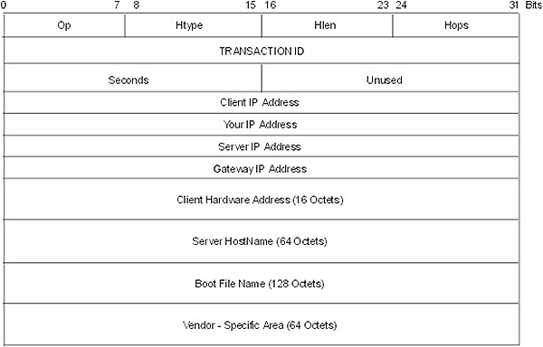
BootP frame
- Op: 8 bits
The message type, 1 = BOOTREQUEST, 2 = BOOTREPLY - Htype: 8 bits
Same as for ARP/RARP - Hlen: 8 bits
Same as for ARP/RARP - Hops: 8 bits
Used by relay agents when booting via a relay agent. A client sets this field to 0. - Transaction ID: 32 bits
(Also called XID). A random tracking number as for the IP and ICMP protocols - Seconds: 16 bits
The seconds elapsed since the client started to boot - Client IP address: 32 bits
Set by the client to its IP address, or initially to zero - Your IP address: 32 bits
Set by the server to the correct IP address for the client, if the client advertises its IP address as 0 - Server IP address: 32 bits
Server IP address, set by the server - Gateway IP address: 32 bits
The Gateway (router) address, set by the relay agent - Client hardware address: 16 bytes
The client MAC address, set by itself - Server host name: 64 bytes
An optional server name, e.g . Garfield or Computer10 (i.e. the NetBIOS name on a Windows machine) - Boot file name: 128 bytes
Used by the server to return a fully qualified directory path name to the client, e.g. c:\windows\bootfiles\startup.exe. This is the location on the server from which the boot file has to be downloaded - Vendor-specific area: 64 bytes
DHCP options as per RFC 1531
RFC 1532 and RFC 1533 contain subsequent clarifications and extensions to BOOTP.
8.11 DHCP
The Dynamic Host Configuration Protocol, as defined by RFC 1533, 1534, 1541 and 1542, was developed out of BOOTP in order to centralize and streamline the allocation of IP addresses. DHCP’s purpose is to centrally control IP-related information and eliminate the need to manually keep track of the allocation of individual IP addresses.
When TCP/IP starts up on a DHCP-enabled host, a request is broadcast requesting an IP address and a subnet mask. The DHCP server, upon hearing the request, checks its internal database and replies with an IP address. DHCP can also respond with a default gateway address, DNS address(es), or the address of a NetBIOS name server such as a WINS server. When the IP offer is accepted, it is extended to the client for a specified period of time, called a lease. If the DHCP server runs out of IP addresses, no IP addressing information can be offered to the clients, causing TCP/IP initialization to fail.
DHCP’s advantages include the following:
- It is inexpensive. The server software comes built into many operating systems, and the manual effort involved in managing large numbers of IP addresses is reduced
- IP configuration information is entered electronically by another system, eliminating the possibility of human error
- IP becomes a ‘plug and play operation’
It does, however, have some drawbacks such as:
- A new user may randomly (delinquently) enter a fixed IP address on his computer in order to gain immediate access to the network. That number may subsequently be assigned by DHCP to a different user and show up as a duplicate
- Because the initial input for IP addresses, subnet masks, gateways, DNS addresses, and NetBIOS name server address is done manually, it can easily be entered incorrectly and will affect all hosts relying on the DHCP service
- Exclusive reliance on the DHCP server during the TCP/IP initialization phase could result in an initialization failure if that server is down, or otherwise unavailable
- Certain applications of TCP/IP, such as logging in to a remote network through a firewall, require the use of a specific IP address. DHCP allows for exclusions that prevent certain IP address ranges from being used. If the specific IP address that is needed for remote login has been excluded, the user has a problem
8.11.1 DHCP operation
IP lease request
This is the first step in obtaining an IP address under DHCP. It is initiated by a TCP/IP host, configured to obtain an IP address automatically when booting up. Since the requesting host is not aware of its own IP address, or that belonging to the DHCP server, it will use 0.0.0.0 and 255.255.255.255 respectively. This is known as a ‘DHCP discover’ message. The broadcast is created with UDP ports 67 (BOOTP client) and 68 (BOOTP server). This message contains the MAC address and NetBIOS name for the client system to be used in the next phase of sending a lease offer. If no DHCP server responds, the client may try several times before giving up and resorting to other tactics, such as APIPA (Automatic IP Address Allocation) if supported by the Operating System. APIPA will allow the machine to assume an IP address in the range 169.254/16.
IP lease offer
The second phase involves the actual information given by all DHCP servers that have valid addressing information to offer. Their offers consist of an IP address, subnet mask, lease period (in seconds), and the IP address of the proposing DHCP server. These offers are sent to the requesting client’s MAC address. The pending IP address offer is reserved temporarily to prevent it from being taken simultaneously by other machines, which would otherwise create chaos. Since multiple DHCP servers can be configured, it also adds a degree of fault tolerance, should one of the DHCP servers go down.
IP lease selection
During this phase, the client machine selects the first IP address offer it receives. The client replies by broadcasting an acceptance message, requesting to lease IP information. Just as in stage one, this message will be broadcast as a DHCP request, but this time, it will additionally include the IP address of the DHCP server of which the offer was accepted. All other DHCP servers will then revoke their offers.
IP lease acknowledgment
The accepted DHCP server proceeds to assign an IP address to the client and then sends an acknowledgement message, called a DHCPACK, back to the client. Occasionally, a negative acknowledgment, called a DHCPNACK, is returned. This type of message is most often generated if the client is attempting to re-lease its old IP address, which has since been reassigned elsewhere. Negative acceptance messages can also mean that the requesting client has an inaccurate IP address, resulting from physically changing locations to an alternate subnet.
After this final phase has been successfully completed, the client machine integrates the new IP information into its TCP/IP configuration. It is then usable with all utilities, as if it has been manually entered into the client host.
Lease renewal:
Regardless of the length of time an IP address is leased, the leasing client will send a DHCPREQUEST to the DHCP server when its lease period has elapsed by 50%. If the DHCP server is available, and there are no reasons for rejecting the request, a DHCP acknowledge message is sent to the client, updating the configuration and resetting the lease time. If the server is unavailable, the client will receive an ‘eviction’ notice stating that it had not been renewed. In this event, that client would still have a remaining 50% lease time, and would be allowed full usage privileges for its duration. The rejected client would react by sending out an additional lease renewal attempt when 87.5% of its lease time had elapsed. Any available DHCP server could respond to this DHCPREQUEST message with a DHCPACK, and renew the lease. However, if the client received a DHCPNACK (negative) message, it would have to stop using the IP address immediately, and start the leasing process over, from the beginning.
Lease release
If the client elects to cancel the lease, or is unable to contact the DHCP server before the lease elapses, the lease is automatically released.
Note that DHCP leases are not automatically released at system shutdown. A system that has lost its lease will attempt to re-lease the same address that it had previously used.
The DHCP message format is based on the BOOTP format, and is illustrated in Fig 8.11.

DHCP message format
The fields are as follows:
- Op: 8 bits
The message type, 1 = BOOTREQUEST, 2 = BOOTREPLY - Htype: 8 bits
Same as for ARP/RARP - Hlen: 8 bits
Same as for ARP/RARP - Hops: 8 bits
Used by relay agents when booting via a relay agent. A client sets this field to 0 - Transaction ID: 32 bits
(Also called XID). A random tracking number as for the IP and ICMP protocols - Seconds: 16 bits
The seconds elapsed since the client started to boot - Flags: 16 bits
This field contains a 1-bit broadcast flag, as described in RFC 1531 - Client IP address (ciaddr): 32 bits
Set by the client to its IP address, or initially to zero - Your IP address (yiaddr): 32 bits
Set by the server to the correct IP address for the client, if the client advertises its IP address as 0 - Server IP address (siaddr): 32 bits
Server IP address, set by the server - Gateway IP address (giaddr): 32 bits
The gateway (router) address, set by the relay agent - Client hardware address (chaddr): 16 bytes
The clients MAC address set by itself - Server name (sname): 64 bytes
An optional server name, e.g. Garfield or Computer10 - Boot file name: 128 bytes
Used by the server to return a fully qualified directory path name to the client, e.g. c:\windows\bootfiles\startup.exe. This is the location on the server from which the boot file has to be downloaded - Options: Up to 312 bytes
DHCP options as per RFC 1531
Objectives
When you have completed study of this chapter you should able to apply the following utilities:
- PING
- ARP
- NETSTAT
- NBTSTAT
- IPCONFIG
- WINIPCFG/WNTIPCFG
- TRACERT
- ROUTE
9.1 Introduction
The TCP/IP utilities are mentioned throughout the book. This section is designed to bring them all together in one section for ease of reference, as they are very important in network management and troubleshooting.
Most of the older utilities are DOS-based. However, many sophisticated Windows-based utilities are available nowadays, many of them as freeware or shareware.
9.2 PING
PINGing is one of the easiest ways to test connectivity across the network and confirm that an IP address is reachable. The DOS ping utility (ping.exe) uses ICMP to forward an Echo Request message to the destination address. The destination then responds with an ICMP Echo Reply message. Although the test seems trivial at first sight, it is a powerful diagnostic tool and can demonstrate correct operation between the Internet layers of two hosts across a WAN regardless of the distance and number of intermediate routers involved.
Technically speaking the PING utility can only target an IP address and not, for example, a NetBIOS name or domain name. This is due to the fact that the ICMP messages are carried within IP datagrams, which require the source and destination IP addresses in their headers. Without this feature it would have been impossible to ping across a router. If, therefore, the user does not know the IP address of the target host, the name resolver on the local host has to look it up e.g. via the Domain Name System or in the HOSTS file.
The IP datagram, in turn, is transported by means of a Network Interface layer frame (e.g. Ethernet), which requires, in its header, the MAC addresses of the sender and the next recipient on the local network. If this is not to be found in the ARP cache, the ARP protocol is invoked in order to obtain the MAC address. The result of this action (the mapping of MAC address against IP address) is then stored in the ARP cache. The easiest way to get an overall impression of the process is to capture the events described here by means of a protocol analyzer.
If the IP address is known, the following format can be used:
- ping <IP Address> e.g. ping 192.100.100.4
The command ping 192.100.100.255 will, unfortunately, not cause all hosts on network 192.100.100.0 to be pinged; they have to be accessed one by one.
If the IP address is unknown, one of the following ways can be used to define the target machine:
- ping <NetBIOS name> e.g. ping computer1
This can be done provided computer1’s IP address has already been resolved by NetBIOS - ping <own machine> e.g. ping 127.0.0.1
This is a reserved IP address for loopback testing - ping <own machine> e.g. ping localhost
This is a reserved name for loopback testing, stored in the HOSTS file - ping <domain name> e.g. ping www.idc-online.com
This will be resolved by the Domain Name System
There are several options (switches) available under the ping command, as shown below:
C:\WINDOWS>ping
Usage: ping [-t] [-a] [-n count] [-l size] [-f] [-i TTL] [-v TOS] [-r count] [-s count] [[-j host-list][-k host-list]][-w timeout] destination-list
Options
|
Ping the specified host until stopped To see statistics and continue – type Control-Break To stop – type Control-C |
||
|
Resolve addresses to hostnames | ||
|
count | Number of echo requests to send | |
|
size | Send buffer size | |
|
Set don’t fragment flag in packet | ||
|
TTL | Time To Live | |
|
TOS | Type of service | |
|
count | Record route for count hops | |
|
count | Time-stamp for count hops | |
|
host-list | Loose source route along host-list | |
|
host-list | Strict source route along host-list | |
|
timeout | Timeout in milliseconds to wait for each reply | |
The following examples show how some of the ping options can be applied:
- ping 193.2.45.66 -t will ping the specified IP address repetitively until stopped by typing Ctrl-C
- ping 193.2.45.66 -n 10 will ping the specified IP address 10 times instead of the default of 4
- ping 193.2.45.66 -l 3500 will ping the specified IP address with 3500 bytes of data instead of the 32 byte default message
Here are some examples of what could be learnt by using the ping command.
Example 1: A host with IP address 207.194.66.100/24 is being ‘pinged’ by another host on the same subnet, i.e. with the same NetID. Note that the screen display differs between operating systems, although the basic parameters are the same.
The following response is obtained:
C:\WINDOWS>ping 207.194.66.100
Pinging 207.194.66.100 with 32 bytes of data:
Reply from 207.194.66.100: bytes=32 time<10ms TTL=128
Reply from 207.194.66.100: bytes=32 time=1ms TTL=128
Reply from 207.194.66.100: bytes=32 time=1ms TTL=128
Reply from 207.194.66.100: bytes=32 time=1ms TTL=128
Ping statistics for 207.194.66.100:
Packets: Sent = 4, Received = 4, Lost = 0 (0% loss),
Approximate round trip times in milliseconds:
Minimum = 0ms, Maximum = 1ms, Average = 0ms
C:\WINDOWS>
From the result, the following can be observed:
- The ICMP message contained 32 bytes
- The average RTT (Round Trip Time) to the target host and back is in the vicinity of 1 millisecond
- The TTL (Time To Live) remaining in the IP header after its return is 128. Since TTL is normally set at 128, by the responding host, it can be safely assumed that the TTL value was not altered, and hence there are no routers between the source and destination hosts
Example 2: A host with IP address 207.194.66.101/24 is now ‘pinged’. Although this host is, in fact, nonexistent, it seems legitimate since the NetIDs match. The originating host will therefore attempt a ping, but a timeout will occur.
C:\WINDOWS>ping 207.194.66.101
Pinging 207.194.66.101 with 32 bytes of data:
Request timed out.
Request timed out.
Request timed out.
Request timed out.
Ping statistics for 207.194.66.101:
Packets: Sent = 4, Received = 0, Lost = 4 (100% loss),
Approximate round trip times in milliseconds:
Minimum = 0ms, Maximum = 0ms, Average = 0ms
C:\WINDOWS>
Example 3. As before, but this time the NetID differs i.e. the target host is assumed to reside on a different network. Since, in this case, no default gateway has been specified, the originating host does not even attempt to issue an ICMP message, and immediately issues a ‘host unreachable’ response.
C:\WINDOWS>ping 208.194.66.100
Pinging 208.194.66.100 with 32 bytes of data:
Destination host unreachable.
Destination host unreachable.
Destination host unreachable.
Destination host unreachable.
Ping statistics for 208.194.66.100:
Packets: Sent = 4, Received = 0, Lost = 4 (100% loss),
Approximate round trip times in milliseconds:
Minimum = 0ms, Maximum = 0ms, Average = 0ms
C:\WINDOWS>
The (DOS) PING command is not particularly ‘user friendly’. It is, for example, not possible to ping a large number of hosts sequentially. There are, however, several Windows-based Ping utilities available as freeware or shareware, of which TJPingPro is an example.
The following example shows how a block of contiguous IP addresses can be pinged with a single ‘click’, after setting up ‘start’ and ‘end’ IP addresses on the options screen.

TJPingPro sequential scan (courtesy of Top Jimmy Software)
9.3 ARP
The ARP utility (arp.exe) is used to display the ARP cache that holds the IP to MAC address translation table of hosts on the local subnet. This utility is not to be confused with the Address Resolution Protocol that actually determines the IP to MAC address translation. The ARP utility can also be used to manually add entries to the cache, using the -s option.
C:\WINDOWS>arp
Displays and modifies the IP-to-physical address translation tables used by address resolution protocol (ARP).
| ARP -s | inet_addr eth_addr [if_addr] ARP -d inet_addr [if_addr] ARP -a [inet_addr] [-N if_addr] |
| -a | Displays current ARP entries by interrogating the current protocol data. If inet_addr is specified, the IP and physical addresses for only the specified computer are displayed. If more than one network interface uses ARP, entries for each ARP table are displayed. |
| -g | Same as -a. |
| inet_addr | Specifies an Internet address. |
| -N if_addr | Displays the ARP entries for the network interface specified by if_addr. |
| -d | Deletes the host specified by inet_addr. |
| -s | Adds the host and associates the Internet address inet_addr with the physical address eth_addr. The physical address is given as 6 hexadecimal bytes separated by hyphens. The entry is permanent. |
| eth_addr | Specifies a physical address. |
| if_addr | If present, this specifies the Internet address of the interface whose address translation table should be modified. If not present, the first applicable interface will be used. |
Example:
> arp -s 157.55.85.212 00-aa-00-62-c6-09 …Adds a static entry.
> arp –a …. Displays the arp table.
The following shows a typical display in response to the arp -a command. Note the third column, which indicates type. Entries in the arp cache can be entered manually as static entries, but that poses a problem as IP addresses can be changed and physical network cards (and hence MAC addresses) can be swapped, rendering the stored IP to MAC address mapping useless unless updated. For this reason the ARP protocol binds IP addresses and physical (MAC) addresses in a temporary (i.e. dynamic) way. Dynamic entries are deleted from the cache after a few minutes, unless used.
C:\WINDOWS>arp -a
Interface: 0.0.0.0 on Interface 0x1000002
Internet Address Physical Address Type 192.100.100.7 00-00-c6-f6-34-43 static 192.100.100.99 00-00-fe-c6-57-a8 dynamic C:\WINDOWS>
9.4 NETSTAT
This is used for obtaining protocol statistics and current active connections using TCP/IP. Nowadays there are many Windows-based utilities that can do much more; yet in an emergency NETSTAT is certainly better than nothing at all. Here follows the NETSTAT options.
C:\WINDOWS>netstat /?
Displays protocol statistics and current TCP/IP network connections.
NETSTAT [-a] [-e] [-n] [-s] [-p proto] [-r] [interval]
| -a | Displays all connections and listening ports. |
| -e | Displays Ethernet statistics. This may be combined with the -s option. |
| -n | Displays addresses and port numbers in numerical form. |
| -p proto | Shows connections for the protocol specified by proto; proto may be TCP or UDP. If used with the -s option to display per-protocol statistics, proto may be TCP, UDP, or IP. |
| -r | Displays the routing table. |
| -s | Displays per-protocol statistics. By default, statistics are shown for TCP, UDP and IP; the -p option may be used to specify a subset of the default. |
| interval | Re-displays selected statistics, pausing interval seconds between each display. Press CTRL+C to stop re-displaying statistics. If omitted, netstat will print the current configuration information once. |
| C:\WINDOWS> |
In response to the netstat -e command the following packet and protocol statistics are displayed. This is a summary of events on the network since the last re-boot.
| C:\WINDOWS>netstat -e | ||
| Interface Statistics | ||
| Received | Sent | |
| Bytes | 2442301 | 1000682 |
| Unicast packets | 4769 | 3776 |
| Non-unicast packets | 113 | 4566 |
| Discards | 0 | 0 |
| Errors | 0 | 0 |
| Unknown protocols | 19 | |
| C:\WINDOWS> |
The ‘-p’ option is also helpful as it shows the current connections for a given protocol. For example, C:\>netstat –p tcp shows the current TCP connections
9.5 NBTSTAT
This provides protocol statistics and current TCP/IP connections using NBT (NetBIOS over TCP/IP).
C:\WINDOWS>nbtstat /?
Displays protocol statistics and current TCP/IP connections using NBT (NetBIOS over TCP/IP).
NBTSTAT [-a RemoteName] [-A IP address] [-c] [-n] [-r]
[-R] [-s] [S] [interval] ]
| -a | (adapter status) Lists the remote machine’s name table given its name |
| -A | (Adapter status) Lists the remote machine’s name table given its IP address. |
| -c | (cache) Lists the remote name cache including the IP addresses |
| -n | (names) Lists local NetBIOS names. |
| -r | (resolved) Lists names resolved by broadcast and via WINS |
| -R | (Reload) Purges and reloads the remote cache name table |
| -S | (Sessions) Lists sessions table with the destination IP addresses |
| -s | (sessions) Lists sessions table converting destination IP addresses to host names via the hosts file. |
| RemoteName | Remote host machine name. |
| IP address | Dotted decimal representation of the IP address. |
| Interval | Re-displays selected statistics, pausing interval seconds between each display. Press Ctrl+C to stop re-displaying statistics. |
| C:\WINDOWS> |
9.6 IPCONFIG
This shows the entire TCP/IP configuration present in a host. It also has the additional versatility of interfacing with a DHCP server to renew a leased IP address.
IPCONFIG will return, amongst other things, the host’s IP address, its subnet mask and default gateway.
C:\WINDOWS>ipconfig /?
Windows 98 IP Configuration
Command line options:
/All – Display detailed information. /Batch [file] – Write to file or ./WINIPCFG.OUT /renew_all – Renew all adapters. /release_all – Release all adapters. /renew N – Renew adapter N. /release N – Release adapter N. C:\WINDOWS>
An option often used is ipconfig /all. This command will display the configuration details of all NICs as well as that of the dial-up connection.
Note that IPCONFIG will list the generic name of the adapter. Therefore, a 3010 3Com US Robotics 56K modem is simply listed as a PPP adapter, while a Linksys Ethernet 10BaseT/10Base2 Combo PCMCIA card is listed as a generic Novell 2000 adapter.
C:\WINDOWS>ipconfig /all
Windows 98 IP Configuration
Host Name . . . . . . . . . : COMPUTER100 DNS Servers . . . . . . . . : Node Type . . . . . . . . . : Broadcast NetBIOS Scope ID. . . . . . : IP Routing Enabled. . . . . : No WINS Proxy Enabled. . . . . : No NetBIOS Resolution Uses DNS : No
0 Ethernet adapter :
Description . . . . . . . . : PPP Adapter. Physical Address. . . . . . : 44-45-53-54-00-00 DHCP Enabled. . . . . . . . : Yes IP Address. . . . . . . . . : 0.0.0.0 Subnet Mask . . . . . . . . : 0.0.0.0 Default Gateway . . . . . . : DHCP Server . . . . . . . . : 255.255.255.255 Primary WINS Server . . . . : Secondary WINS Server . . . : Lease Obtained. . . . . . . : Lease Expires . . . . . . . :
1 Ethernet adapter :
Description . . . . . . . . : Novell 2000 Adapter. Physical Address. . . . . . : 00-E0-98-71-57-AF DHCP Enabled. . . . . . . . : No IP Address. . . . . . . . . : 207.194.66.100 Subnet Mask . . . . . . . . : 255.255.255.224 Default Gateway . . . . . . : Primary WINS Server . . . . : Secondary WINS Server . . . : Lease Obtained. . . . . . . : Lease Expires . . . . . . . :
C:\WINDOWS>
9.7 WINIPCFG/WNITPCFG
WINIPCFG (Windows IP Configuration for Windows 95/98) and WNTIPCFG (Windows NT IP Configuration for NT, 2000 and XP) provide the same information as IPCONFIG, but in a Windows format. Like IPCONFIG, it is capable to force a DHCP server into releasing and re-issuing leased IP addresses.

WNTIPCFG configuration display (courtesy Microsoft Corporation)
Click the ‘more details’ tab for an expanded view.
9.8 TRACE RouTe
This is often used to trace a specific TCP/IP communications path. The spelling of the command varies slightly. For UNIX it is traceroute, for Windows it is tracert.
The following figure shows the TRACERT options.
C:\WINDOWS>tracert
Usage: tracert [-d] [-h maximum_hops] [-j host-list] [-w timeout] target_name
Options:
| -d | Do not resolve addresses to hostnames. |
| -h maximum_hops | Maximum number of hops to search for target. |
| -j host-list | Loose source route along host-list. |
| -w timeout | Wait timeout milliseconds for each reply. |
C:\WINDOWS>
Here follows a route trace from Perth, Australia, to a server in the USA.
C:\WINDOWS>tracert www.idc-online.com
Tracing route to www.idc-online.com [216.55.154.228] over a maximum of 30 hops:
| 1 | 169ms 160ms 174ms slip202-135-15-3-0.sy.au.ibm.net [202.135.15.30] |
| 2 | 213ms 297ms 296ms 152.158.248.250 |
| 3 | 624ms 589ms 533ms sfra1sr1-2-0-0-5.ca.us.prserv.net [165.87.225.46] |
| 4 | 545ms 535ms 628ms sfra1sr2-101-0.ca.us.prserv.net [165.87.33.185] |
| 5 | 564ms 562ms 573ms 165.87.160.193 |
| 6 | 558ms 564ms 573ms 114.ATM3-0.XR1.SFO1.ALTER.NET [146.188.148.210] |
| 7 | 574ms 701ms 555ms 187.at-2-10.TR1.SAC1.ALTER.NET [152.63.50.230] |
| 8 | 491ms 480ms 500ms 127.at-6-10.TR1.LAX9.ALTER.NET [152.63.5.101] |
| 9 | 504ms 534ms 511ms 297.ATM7-0.XR1.LAX2.ALTER.NET [152.63.112.149] |
| 10 | 500ms 478ms 491ms 195.ATM9-0-0.GW2.SDG1.ALTER.NET [146.188.249.81] |
| 11 | 491ms 564ms 584ms anet-gw.customer.ALTER.NET [157.130.224.154] |
| 12 | 575ms 554ms 613ms www.idc-online.com [216.55.154.228] |
Trace complete.
C:\WINDOWS>
As is often the case, the DOS approach is not the most user-friendly option. Notice the result when the same type of trace (albeit to a different address) is done with TJPingPro. The same TCP/IP protocols are still used, but now they are accessed through a third-party application program.

TJPingPro trace (courtesy of Top Jimmy Software)
The most comprehensive tracing is, however, done via application programs such as Neotrace. The following figures give some of the results of a trace to the same location used for the previous two examples.

NeoTrace display (courtesy NeoWorx Inc)
9.9 ROUTE
Even a single-homed host needs to make routing decisions. These are made on the basis of information contained in the route table. This table is automatically built by Windows on the basis of the hosts’s IP configuration. The ROUTE command can be used to manually configure network routing tables on TCP/IP hosts. This may be a tedious task but is sometimes necessary for reasons of security or because a specific route has to be added.
The following shows the route command options (switches).
C:\WINDOWS>route /?
Manipulates network routing tables.
ROUTE [-f] [command [destination] [MASK netmask] [gateway] [METRIC metric]]
-f Clears the routing tables of all gateway entries. If this is used in conjunction with one of the commands, the tables are cleared prior to running the command. command Must be one of four: Prints a route ADD Adds a route DELETE Deletes a route CHANGE Modifies an existing route destination Specifies the destination host. MASK Specifies that the next parameter is the ‘netmask’ value. netmask Specifies a subnet mask value to be associated with this route entry. If not specified, it defaults to 255.255.255.255. METRIC Specifies that the next parameter metric’ is the cost for this destination
All symbolic names used for destination are looked up in the network database file NETWORKS. The symbolic names for gateway are looked up in the host name database file HOSTS.
If the command is PRINT or DELETE, wildcards may be used for the destination and gateway, or the gateway argument may be omitted.
Diagnostic notes:
Invalid MASK generates an error, that is when (DEST & MASK) != DEST.
Example> route ADD 255.0.0.0 157.0.0.0 MASK 155.0.0.0
157.55.80.1
The route addition failed: 87
Examples:
> route PRINT
> route ADD 157.0.0.0 MASK 255.0.0.0 157.55.80.1 METRIC 3
^destination ^mask ^gateway ^metric
> route PRINT
> route DELETE 157.0.0.0
> route PRINT
C:\WINDOWS>
The route table resides on all TCP/IP hosts and is not to be confused with the routing table maintained by individual routers, as the exact details of these depend on the routing protocol used by the router, such as RIP or OSPF. An individual entry is read from left to right as follows: ‘If a message is destined for network 157.0.0.0, with subnet mask 255.0.0.0, then route it through to the gateway (router) address 157.55.80.1’. Remember that a HostID equal to 0, as used here, does not refer to a specific host but rather to a network as a whole. The ‘metric’ is a yardstick for making routing decisions. The calculation thereof is a topic on its own, but in the simplest case it could represent ‘hops’. Any destination on the local network is one hop, with one hop added for each additional router to be traversed.
Routes can also be added with the route add and route delete commands.
Route add 192.100.100.0 mask 255.255.255.0 192.100.100.1 will add a route and route delete 192.100.100.0 will delete a particular route. Manual adding of routes are sometimes necessary, for example in the case where the installation of dial-up proxy server software on a given host overwrites the existing default gateway setting on that host in order to ‘point’ to the ISP’s default gateway. This makes it impossible for the host to reach an existing adjacent network across the intermediate router, unless a manual entry is made. If said entry ‘does the job’ but disappears when the host is re-booted, the appropriate route command needs to be included in the autoexec.bat file or made persistent if that option is available for the operating system being used, through the use of the [-p] switch.
The following response was obtained from the route print command.
| Active routes: | ||||
| Network Address | Netmask | Gateway Address | Interface | Metric |
| 127.0.0.0 | 255.0.0.0 | 127.0.0.1 1 | 27.0.0.1 | 1 |
| 207.194.66.96 | 255.255.255.224 | 207.194.66.100 | 207.194.66.100 | 1 |
| 207.194.66.100 | 255.255.255.255 | 127.0.0.1 | 127.0.0.1 | 1 |
| 207.194.66.255 | 255.255.255.255 | 207.194.66.100 | 207.194.66.100 | 1 |
| 224.0.0.0 | 224.0.0.0 | 207.194.66.100 | 207.194.66.100 | 1 |
| 255.255.255.255 | 255.255.255.255 | 207.194.66.100 | 0.0.0.0 | 1 |
| C:\WINDOWS.000> |
The first column, Network Address, is the destination and can contain the host address, the subnet address, the network address or the default gateway. The search order is in this sequence, from host address (most unique route) to default gateway (most generic). In the example above:
- 0.0.0.0 is the default route
- 127.0.0.0 is the loopback address
- 207.194.66.96 is the local subnet address
- 207.194.66.100 is the network card (NIC) address
- 207.194.66.255 is the subnet broadcast address
- 224.0.0.0 is the multicast address
- 255.255.255.255 is the limited broadcast address
The netmask dictates what portion of the destination IP address must match the Network Address for a specific route to be used. When the Network Address and Netmask are written in binary, then where the Netmask is a ‘1’ the destination address must match the Network address, but where the Netmask is ‘o’ they need not match.
9.10 The HOSTS file
The HOSTS file is used on UNIX and Windows systems to resolve the mapping of a ‘name’ (any given name) to an IP address.
The following is an example of a typical Windows hosts file. The file (‘hosts’) is located in c:\WINNT\system32\drivers\etc for Windows 2000 and C:\Windows\drivers\etc for XP. If a user is uncertain about the correct format of the entries, a sample file is stored in the same folder as hosts.sam. As a matter of convenience the hosts.sam file can be edited as in the accompanying example, but it MUST then be saved as hosts only, i.e. without the ‘.sam’ extension.
In the example, host 192.100.100.2 can be interrogated by typing ping john.
The following is the contents of the Windows XP hosts file.
- # Copyright (c) 1993-1999 Microsoft Corp.
- #
- # This is a sample HOSTS file used by Microsoft TCP/IP for Windows.
- #
- # This file contains the mappings of IP addresses to host names. Each
- # entry should be kept on an individual line. The IP address should
- # be placed in the first column followed by the corresponding host name.
- # The IP address and the host name should be separated by at least one
- # space.
- #
- # Additionally, comments (such as these) may be inserted on individual
- # lines or following the machine name denoted by a ‘#’ symbol.
- #
- # For example:
- #
- # 102.54.94.97 rhino.acme.com
- # source server
- # 38.25.63.10 x.acme.com
- # x client host
- 127.0.0.1 localhost
- 192.100.100.2 john
Objectives
When you have completed this chapter you should be able to:
- Explain the basic function of each of the devices listed under 10.1
- Explain the fundamental differences between the operation and application of switches, bridges and routers
10.1 Introduction
In the design of an Ethernet system there are a number of different components to be used. These include:
- Repeaters
- Media converters
- Bridges
- Hubs
- Switches
- Routers
- Gateways
- Print servers
- Terminal servers
- Remote Access Servers
- Time servers
- Thin servers
The lengths of LAN segments are limited due to physical and/or collision domain constraints and there is often a need to increase this range. This can be achieved by means of a number of interconnecting devices, ranging from repeaters to gateways. It may also be necessary to partition an existing network into separate networks for reasons of security or traffic overload.
In modern network devices the functions mentioned above are often mixed:
- A shared hub is, in fact, a multi-port repeater
- A layer 2 switch is essentially a multi-port bridge
- Segmentable and dual-speed shared hubs make use of internal bridges
- Switches can function as bridges, a two-port switch being none other than a bridge
- Layer 3 switches function as routers
These examples are not meant to confuse the reader, but serve to emphasize the fact that the functions should be understood, rather than the ‘boxes’ in which they are packaged.
10.2 Repeaters
A repeater operates at the Physical layer of the OSI model (layer 1) and simply retransmits incoming electrical signals. This involves amplifying and re-timing the signals received on one segment onto all other segments, without considering any possible collisions. All segments need to operate with the same media access mechanism and the repeater is unconcerned with the meaning of the individual bits in the packets. Collisions, truncated packets or electrical noise on one segment are transmitted onto all other segments.
Repeaters are only used in legacy (CSMA/CD) Ethernet networks as they are not required in modern switched networks.
10.2.1 Packaging
Repeaters are packaged either as stand-alone units (i.e. desktop models or small cigarette package-sized units) or 19-inch rack-mount units. Some of these can link two segments only, while larger rack-mount modular units (called concentrators) are used for linking multiple segments. Regardless of packaging, repeaters can be classified either as local repeaters (for linking network segments that are physically in close proximity), or as remote repeaters for linking segments that are some distance apart.

Repeater application
10.2.2 Local Ethernet repeaters
Several options are available:
- Two-port local repeaters offer various combinations of the various Physical layer alternatives, such as 10BaseFL/10BaseFL. By using such devices (often called boosters or extenders) one can, for example, extend the distance between a computer and a 10BaseT Hub by up to 100m, or extend a 10BaseFL link between two devices (such as bridges) by up to 2 km with multimode fiber, or 15 km with single mode fiber.
- Multi-port local repeaters are also available as chassis-type units; i.e. as frames with common backplanes and removable units. An advantage of this approach is that, for example, 10Base2, 10Base5, 10BaseT and 10BaseFL can be mixed in one unit, with an option of SNMP management for the overall unit. These are also referred to as concentrators
10.2.3 Remote repeaters
Remote repeaters, on the other hand, have to be used in pairs with one repeater connected to each network segment and a fiber-optic link between the repeaters. On the network side they typically offer 10/100Base-T options. On the interconnecting side the choices include ‘single pair Ethernet’, using telephone cable up to several hundred meters in length, or single mode/multi-mode optic fiber, with various connector options. With 10BaseFL (backwards compatible with the old FOIRL standard), this distance can be up to 1.6 km bit with current technology single mode fiber links available up to several tens of kilometers.
Although repeaters are probable the cheapest way to extend a network, they do so without separating collision domains, or network traffic. They simply extend the physical size of the network. All segments joined by repeaters therefore share the same bandwidth and collision domain.
10.3 Media converters
Media converters are essentially repeaters, but interconnect mixed media viz. copper and fiber. An example would be 10BaseT/ 10BaseFL. As in the case of repeaters, they are available in single and multi-port options, and in stand-alone or chassis type configurations. The latter option often features remote management via SNMP.

Media converter application
Models may vary between manufacturers, but generally Ethernet media converters support:
- 10 Mbps (10Base2, 10BaseT, 10BaseFL- single and multi-mode)
- 100 Mbps (Fast) Ethernet (100Base-TX, 100Base-FX- single and multimode)
- 1000 Mbps (Gigabit) Ethernet (single and multimode)
Distances supported are typically 2 km for 10BaseFL, 5 km for 100Base-FX (multimode) and 40 Km for 100Base-SX (single mode). An added advantage of the fast and Gigabit Ethernet media converters is that they support full duplex operation, which effectively doubles the available bandwidth.
10.4 Bridges
Bridges operate at the Data Link layer of the OSI model (layer 2) and are used to interconnect two separate networks to form a single large continuous LAN. From a TCP/IP perspective, however, the overall network still remains one network with a single NetID. The bridge only divides the network up into two segments, each with its own collision domain and each retaining its full (say, 10 Mbps) bandwidth. Broadcast transmissions are seen by all nodes, on both sides of the bridge.
The bridge exists as a node on each network, although it does not have a MAC address of its own, and passes only valid messages across to destination addresses on the other network. The decision as to whether or not a frame should be passed across the bridge is based on the layer 2 address, i.e. the media (MAC) address. The bridge examines the destination MAC addresses of all frames on both sides to determine whether they should be forwarded across the bridge or not.
Bridges can be classified either as MAC or LLC bridges, the MAC sub-layer being the lower half of the Data Link layer and the LLC sub-layer being the upper half. For MAC bridges the media access control mechanism on both sides must be identical; thus it can bridge only Ethernet to Ethernet, Token Ring to Token Ring and so on. For LLC bridges, the Data Link layer protocol must be identical on both sides of the bridge (e.g. IEEE 802.2 LLC); however, the physical layers or MAC sub-layers do not necessarily have to be the same. Thus the bridge isolates the media access mechanisms of the networks. Data can therefore be transferred, for example, between Ethernet and Token Ring LANs. In this case, collisions on the Ethernet system do not cross the bridge nor do the tokens.
Bridges can be used to extend the length of a network (as with repeaters) but in addition they improve network performance. For example, if a shared (i.e. CSMA/CD) network is demonstrating fairly slow response times, the nodes that mainly communicate with each other can be grouped together on one segment and the remaining nodes can be grouped together in the other segment. The busy segment may not see much improvement in response rates (as it is already quite busy) but the lower activity segment may see quite an improvement in response times. Bridges should be designed so that 80% or more of the traffic remains within the segment and only 20% cross the bridge. Stations generating excessive traffic across the bridge should be identified by a protocol analyzer and relocated to another LAN.
Because bridges are store-and-forward devices, they truncate the collision domains i.e. collisions on one side of the bridge have no relevance on the other side.
10.4.1 Intelligent bridges
Intelligent bridges (also referred to as transparent or spanning-tree bridges) are the most commonly used bridges because they are very efficient in operation and do not need to be taught the network topology. A transparent bridge learns and maintains two address lists corresponding to the networks it is connected to. When the bridge observes a frame from the one Ethernet segment, its source MAC address is added to the list of source addresses for that segment. The destination address is then compared with those on the address list for each segment and a decision is made whether to transmit the frame onto the other segment or not. If no address corresponding with the destination node is recorded in either of these two lists, the message is re-transmitted across the bridge to ensure that the message is delivered to the correct network. When the destination host replies, the bridge becomes aware of its location and updates the lists accordingly. Over a period of time the bridge learns about all the addresses on the network and thus avoids transmitting unnecessary traffic to adjacent segments. The bridge also maintains time-out data for each entry to ensure the table is kept up to date and old entries purged.
Transparent bridges cannot have loops as these could cause endless circulation of packets. If the network contains bridges that could form a loop as shown in Figure 10.3, any redundant paths need to be deactivated.
Refer to Fig 10.1. Assume that bridges A and B have not yet determined the whereabouts of node 2. Node 1 now sends a packet to node 2. Both bridges receive this packet on their ‘1’ inputs (A1 and B1). Since neither of them know where the destination node is, they simultaneously pass the packet to their ‘2’ side (A2 and B2). A2 now detects a broadcast message from B2 and passes it across to A1, since it does not know where the destination is. B2, in similar fashion, detects the broadcast message from A2 and passes it on to B1. The process is repeated and leads to an exponential increase in the number of packets on the network.
In order to solve the problem, the bridges need to communicate amongst themselves and decide on an optimum path between nodes A and B, and disable any redundant path(s). This is achieved by means of the Spanning Tree Algorithm (IEEE 802.1d). The bridges exchange configuration information via Bridge Protocol Data Units (BPDUs) and agree on the optimum path.

Avoidance of loops in bridge networks
10.4.2 Local vs remote bridges
Local bridges have two network ports and hence interconnect two adjacent network segments at one point. This function is currently often performed by switches, being essentially intelligent multi-port bridges.
A very useful type of local bridge is a 10/100 Mbps Ethernet bridge, which allows interconnection of 10BaseT, 100Base-TX and 100Base-FX networks, thereby performing the required speed translation. These bridges typically provide full duplex operation on 100BastTX and 100Base-FX, and employ internal buffers to prevent saturation of the 10BaseT port.
Remote bridges, on the other hand, operate in pairs with some form of interconnection between them. This interconnection can be with or without modems, and include
RS-232, V.35, RS-422, RS-530, X.21, 4-wire, or fiber (both single and multi-mode). The distance between bridges can typically be up to 40 Km.

Remote bridge application
Wireless Ethernet bridges are available from several vendors. They typically transmit at1.5 Mbps and use the 900 MHz band, unlicensed in the USA, Israel and Australia.
10.5 Hubs
Hubs are used to interconnect hosts in a physical star configuration. This section will deal with Ethernet hubs, which are of the 10/100Base-T variety. They are available in many configurations, some of which will be discussed below.
10.5.1 Desktop vs stackable hubs
Smaller desktop units are intended for stand-alone applications, and typically have 5 to 8 ports. Stackable hubs, on the other hand, typically have up to 24 ports and can be stacked and interconnected to act as one large hub without any repeater count restrictions. These stacks are often mounted in 19-inch cabinets.

10BaseThub interconnection
10.5.2 Shared vs switched hubs
Shared hubs interconnect all ports on the hub in order to form a logical bus. This is typical of the cheaper workgroup hubs. All hosts connected to the hub share the available bandwidth since they all form part of the same collision domain.
Although they physically look alike, switched hubs (better known as switches) allow each port to retain and share its full bandwidth only with the hosts connected to that port. Each port (and the segment connected to that port) functions as a separate collision domain. This attribute will be discussed in more detail in the section on switches.
Because of the speed advantages of switches over shared hubs, and the decreasing cost of switches, hubs are seldom used in new applications.
10.5.3 Managed hubs
Managed hubs have an on-board processor with its own MAC and IP address. Once the hub has been set up via a PC on the hub’s serial (COM) port, it can be monitored and controlled via the network using SNMP or RMON. The user can perform activities such as enabling/disabling individual ports, performing segmentation (see next section), monitoring the traffic on a given port, or setting alarm conditions for a given port.
10.5.4 Segmentable hubs
On a non-segmentable shared hub, all hosts share the same bandwidth. On a segmentable hub, however, the ports can be grouped under software control into several shared segments. All hosts on each segment then share the full bandwidth on that segment, which means that a 24-port 10Base-T hub segmented into four groups effectively supports 40 Mbps. The configured segments are internally connected via bridges, so that all ports can still communicate with each other if needed.
10.5.5 Dual-speed hubs
Some hubs offer dual-speed ports, e.g. 10BaseT/100Base-T. These ports are auto-configured, i.e. each port senses the speed of the NIC connected to it, and adjusts its own speed accordingly. All the 10BaseT ports form a common low-speed internal segment, while all the 100Base-T ports form a common high-speed internal segment. The two internal segments are interconnected via a speed-matching bridge.
10.5.6 Modular hubs
Some stackable hubs are modular, allowing the user to configure the hub by plugging in a separate module for each port. Ethernet options typically include both 10 and 100 Mbps, with either copper or fiber. These hubs are sometimes referred to as chassis hubs.
10.5.7 Hub interconnection
Stackable hubs are best interconnected by means of special stacking cables attached to the appropriate connectors on the back of the chassis.
An alternative method for non-stackable hubs is by ‘daisy-chaining’ an interconnecting port on each hub by means of a UTP patch cord. Care has to be taken not to connect the Transmit pins on the ports together (and, for that matter, the receive pins) – it simply will not work. This is similar to interconnecting two COM ports with a ‘straight’ cable i.e. without a null modem. Connect transmit to receive and vice versa by (a) using a crossover cable and interconnecting two ‘normal’ ports, or (b) using a normal (‘straight’) cable and utilizing a crossover port on one of the hubs. Some hubs have a dedicated uplink (crossover) port while others have a port that can be manually switched into crossover mode.
A third method that can be used on older hubs with a 10Base2 port is to create a backbone. Attach a BNC T-piece to each hub, and interconnect the T-pieces with RG-58 coax cable. The open connections on the extreme ends of the backbone obviously have to be terminated.
Fast Ethernet hubs need to be deployed with caution because the inherent propagation delay of the hub is significant in terms of the 5.12 microsecond collision domain size. Fast Ethernet hubs are classified as Class I, II or II+, and the class dictates the number of hubs that can be interconnected. For example, Class II dictates that there may be no more than two hubs between any given pair of nodes, that the maximum distance between the two hubs shall not exceed 5 m, and that the maximum distance between any two nodes shall not exceed 205m. The safest approach, however, is to follow the guidelines of the manufacturer.

Fast Ethernet hub interconnection
10.6 Switches
Ethernet switches are an expansion of the concept of bridging and are, in fact, intelligent (self-learning) multi-port bridges. They allow frame transfers to be accomplished between any pair of devices on a network on a per-frame basis. Only the two ports involved ‘see’ the specific frame. Illustrated below is an example of an 8 port switch, with 8 hosts attached (one attached node per switch port). This comprises a physical star configuration, but it does not operate as a logical bus as an ordinary hub does. Since each port on the switch represents a separate segment with its own collision domain, it means that in this case there are only two devices on each segment, namely the host and the switch port. Hence, in this particular case, there can be no collisions on any segment!
In the sketch below hosts 1 & 7, 3 & 5 and 4 & 8 need to communicate at a given moment, and are connected directly for the duration of the frame transfer. For example, host 7 sends a packet to the switch, which determines the destination address, and directs the package to port 1 at 10 Mbps.

8-Port Ethernet switch
If host 3 wishes to communicate with host 5, the same procedure is repeated. Provided that there are no conflicting destinations, a 16-port switch could allow 8 concurrent frame exchanges at 10 Mbps, rendering an effective bandwidth of 80 Mbps. If the switch allowed full duplex operation, this figure could be doubled.
10.6.1 Cut-through vs store-and-forward
Switches have two basic architectures, viz. cut-through and store-and-forward. In the past, cut-through switches were faster because they examined the packet destination address only before forwarding the frame to the destination segment. A store-and-forward switch, on the other hand, accepts and analyses the entire packet before forwarding it to its destination. It takes more time to examine the entire packet, but it allows the switch to catch certain packet errors and keep them from propagating through the network. The speed of modern store-and-forward switches has caught up with cut-through switches so that the speed difference between the two is minimal. There are also a number of hybrid designs that mix the two architectures.
Since a store-and-forward switch buffers the frame, it can delay forwarding the frame if there is traffic on the destination segment, thereby adhering to the CSMA/CD protocol. In the case of a cut-through switch this could be a problem, since a busy destination segment means that the frame cannot be forwarded, yet it cannot be stored either unless the switch can buffer the packet. On older switches the solution was to force a collision on the source segment, thereby enticing the source host to retransmit the frame.
10.6.2 Layer 2 switches vs layer 3 switches
Layer 2 switches operate at the Data Link layer of the OSI model and derive their addressing information from the destination MAC address in the Ethernet header. Layer 3 switches, on the other hand, obtain addressing information from the Network layer, namely from the destination IP address in the IP header. Layer 3 switches are used to replace routers in LANs as they can do basic IP routing (supporting protocols such as and RIPv2) at almost ‘wire-speed’; hence they are significantly faster than routers. They do not, however, replace ‘real’ routers as Gateways to the WAN.
10.6.3 Full duplex switches
An additional advantage is full duplex Ethernet, where a device can simultaneously transmit AND receive data over one Ethernet connection. This requires an Ethernet NIC as well as a switch that supports full duplex. This enables two devices to transmit and receive simultaneously via a switch. The node automatically negotiates with the switch and uses full duplex if both devices can support it.
Full duplex is useful in situations where large amounts of data are to be moved around quickly, for example between graphics workstations and file servers.
10.6.4 Switch applications
High-speed aggregation
Switches are very efficient in providing a high-speed aggregated connection to a server or backbone. Apart from the normal lower-speed (say, 100Base-TX) ports, switches have a high-speed uplink port (e.g. 1000Base-T). This port is simply another port on the switch, accessible by all the other ports, but features a speed conversion from 10 Mbps to 100 Mbps.
Assume that the uplink port was connected to a file server. If all the other ports (say, eight times 100Base-T) wanted to access the server concurrently, this would necessitate a bandwidth of 800 Mbps in order to avoid a bottleneck and subsequent delays. With a 100Base-TX uplink port this would create a serious problem. However, with a 1000Base-T uplink there is still 200 Mbps of bandwidth to spare.

Using a Switch to connect users to a Server
Backbones
Switches are very effective in backbone applications, linking several hub-based (CSMA/CD) LANs together as one, yet segregating the collision domains. An example could be a switch located in the basement of a building, linking the networks on different floors of the building. Since the actual ‘backbone’ is contained within the switch, it is known in this application as a ‘collapsed backbone’.

Using a switch as a backbone
VLANs and deterministic Ethernet
Provided that a LAN is constructed around switches that support VLANs, individual hosts on the physical LAN can be grouped into smaller Virtual LANs (VLANs), totally invisible to their fellow hosts. Unfortunately, the ‘standard’ Ethernet/ IEEE802.3 header does not contain sufficient information to identify members of each VLAN; hence, the frame had to be modified by the insertion of a ‘tag’ between the Source MAC address and the Type/Length fields. This modified frame is known as an IEEE 802.1Q tagged frame and is used for communication between the switches.
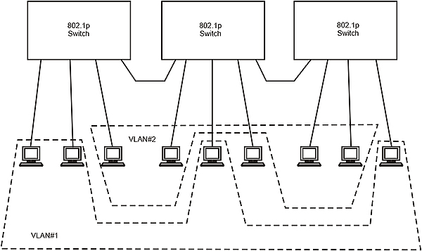
Virtual LANs using switches
The IEEE802.1p committee has defined a standard for packet-based LANs that supports layer 2 traffic prioritization in a switched LAN environment. IEEE802.1p is part of a larger initiative (IEEE802.1p/Q) that adds more information to the Ethernet header (as shown in Fig 10.11) to allow networks to support VLANs and traffic prioritization.

IEEE802.1p/Q modified Ethernet header
802.1p/Q adds 32 bits to the header. Sixteen are used for a unique number (0x8100) to identify the frame as a ‘tagged’ frame, three are for a Priority tag, one is a Canonical Format Indicator (CFI) to indicate whether the MSB of the VLAN ID is on the left or the right, and twelve are for the VLAN ID number. This allows for eight discrete priority layers from 0 (low) to 7 (high), which supports different kinds of traffic in terms of their delay-sensitivity. Since IEEE802.1p/Q operates at layer 2, it supports prioritization for all traffic on the VLAN, both IP and non-IP. This introduction of priority layers enables so-called deterministic Ethernet where, instead of contending for access to a bus, a source node can pass a frame almost immediately to a destination node on the basis of its priority, and without risk of any collisions.
The alternative method for creating a VLAN is a ‘port based VLAN’. On a port-based VLAN switch the user must configure each port to accept packets (only) from certain other ports. Assume ports 1, 2 and 3 on a switch have to be set up as one VLAN. The switch will then be configured as follows:
- Port 1 egress Port 2, egress Port 3
- Port 2 egress Port 1, egress Port 3
- Port 3 egress Port 1, egress Port 2
Ethernet Protected Switched Rings (EPSR)
EPSR is a reliable switching technology to protect the access network aligned with failures in the link, node and equipment of a network. EPSR selects primary and alternate paths for the service traffic. It takes less than 50 msec for failure detection and will switch over to alternate facilities.
EPSR, much like STP (Spanning Tree Protocol) provides a polling mechanism to detect ring-based faults and failover accordingly. It uses a fault detection scheme that alerts the ring about the break and indicates that it must take action. During a fault, the ring automatically heals itself by sending traffic over a protected reverse path.
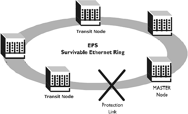
Physical structure of EPSR
Master Node is the controlling node for an EPSR Domain, responsible for status polling, collecting error messages, and controlling the flow of traffic in the Domain. All other nodes are transit nodes. Transit nodes generate failure notices and receive control messages from the Master.
10.7 Routers
Unlike bridges and layer 2 switches, routers operate at layer 3 of the OSI model, viz. the Network layer (or, the Internet layer of the DoD model). They therefore ignore address information contained within the Data Link layer header (the MAC addresses) and, instead, delve deeper into each frame and extract the address information contained in the Network layer. For IP this is the IP address.
Like bridges or switches, routers appear as hosts on the networks to which they are connected. They are connected to each participating network through a NIC, each with its own MAC address and IP address. Each NIC has to be assigned an IP address with the same NetID as that of the network it is connected to. The IP address of the router on each network is known as the Default Gateway for that network and each host on the internetwork requires at least one Default Gateway (but could have more). The Default Gateway is the IP address to which any host on that network must forward a packet if it finds that the NetID of the destination host and the local NetID does not match, which implies remote delivery of the packet.
A second major difference between routers and bridges or switches is that routers will not act autonomously, but instead have to be given the frames that need to be forwarded. Consequently, if the Default Gateway is not configured on a particular host, it is unable to access the router.
Because routers operate at the Network layer, they are used to transfer data between two networks that have the same Internet layer protocols (such as IP) but not necessarily the same Physical layer or Data Link layer protocols. Routers are therefore said to be protocol dependent, and have to be able to handle all the Internet layer protocols present on a particular network. A network using Novell Netware therefore requires routers that can accommodate IPX (Internet Packet exchange) – the Network layer component of SPX/IPX. If this network has to handle Internet access as well, it can only do this via IP, and hence the routers will need to be upgraded to handle both IPX and IP.
Routers maintain tables of the networks that they are connected to and of the optimum path to reach a particular destination network. They then direct the message to the next router along that path.
10.7.1 Two-port vs multi-port routers
Multi-port routers have a modular construction and can interconnect several networks. The most common type of router is, however, a 2-port router. Since these are invariably used to implement WANs, they connect LANs to a ‘communications cloud’; the one port will be a local LAN port e.g. 100Base-TX, but the second port will be a WAN port such as X.25.

Implementing a WAN with 2-port routers
10.7.2 Border routers
Routers within an Autonomous System normally communicate with each other using an Interior Gateway Protocol such as RIP. However, routers on the perimeter of the Autonomous System, which also communicate with remote Autonomous Systems, need to do that via an Exterior Gateway Protocol such as BGP-4. Whilst doing this, they still have to communicate with other routers within their own Autonomous System, e.g. via RIPv2. These routers are referred to as Border Routers.
10.7.3 Routing vs bridging
It sometimes happens that a router is confronted with a layer 3 (Network layer) address it does not understand. In the case of an IP router, this may be a Novell IPX address. A similar situation will arise in the case of NetBIOS/NetBEUI, which is non-routable. A ‘brouter’ (bridging router) will revert to a bridge if it cannot understand the layer 3 protocol, and in this way make a decision as to how to deal with the packet. Most modern routers have this function built in.
10.8 Gateways
Gateways are network interconnection devices, not to be confused with Default Gateways which are the IP addresses of the routers to which packets are forwarded for subsequent routing (indirect delivery).
A gateway is designed to connect dissimilar networks and could operate anywhere from layer 4 to layer 7 of the OSI model. In a worst case scenario, a gateway may be required to decode and re-encode all seven layers of two dissimilar network protocol stacks, for example when connecting an Ethernet network to an IBM SNA network. Gateways thus have the highest overhead and the lowest performance of all the internetworking devices. The gateway translates from one protocol to the other and handles differences in physical signals, data format, and speed.
Since gateways are, per definition, protocol converters, it so happens that a 2-port (WAN) router could also be classified as a gateway since it has to convert both layer 1 and layer 2 on the LAN side (say, Ethernet) to layer 1 and Layer 2 on the WAN side (say, X.25). This leads to the confusing practice of referring to routers as gateways.
10.9 Print servers
Print servers are network nodes through which printers can be made available to all users. Typical print servers cater for both serial and parallel printers. Some also provide concurrent multi-protocol support, which means that they support multiple protocols and will execute print jobs on a first-come first-served basis regardless of the protocol used. Protocols supported could include SPX/IPX, TCP/IP, AppleTalk/EtherTalk, NetBIOS/NetBEUI, or DEC LAT.

Print server applications
10.10 Terminal servers
Terminal servers connect multiple serial (e.g. RS-232) devices such as system consoles, data entry terminals, bar code readers, scanners, and serial printers to a network. They support multiple protocols such as TCP/IP, SPX/IPX, NetBIOS/NetBEUI, AppleTalk and DEC LAT, which means that they not only can handle devices which support different protocols, but can also provide protocol translation between ports.

Terminal server applications
10.11 Thin servers
Thin servers are essentially single-channel terminal servers. They provide connectivity between Ethernet (e.g. 10BaseT/100Base-TX) and any serial devices with RS-232 or RS-485 ports. They implement the bottom 4 layers of the OSI model with Ethernet and layer 3/4 protocols such as TCP/IP, SPX/IPX and DEC LAT.
A special version, the Industrial Thin Server, is mounted in a rugged DIN rail package. It can be configured over one of its serial ports, and managed via Telnet or SNMP. A software redirector package enables a user to remove a serial device such as a weigh-bridge from its controlling computer, locate it elsewhere, then connect it via a Thin Server to an Ethernet network through the nearest available switch or hub. All this is done without modifying any software. The port redirector software makes the computer ‘think’ that it is still communicating to the weighbridge via the COM port while, in fact, the data and control messages to the device are routed via the network.
Industrial Thin Server (courtesy Lantronix)
10.12 Remote Access Servers
A Remote Access Server (RAS) is a device that allows users to dial into a network via analog telephone or ISDN. Typical RASs support between 1 and 32 dial-in users via PPP or SLIP. User authentication can be done, for example, via PAP, CHAP, Radius, Kerberos or SecurID. Some offer dial-back facilities whereby the user authenticates to the server’s internal table, after which the server dials back to the user so that the cost of the connection is carried by the network and not by the remote user.

Remote Access Server application (courtesy Lantronix)
10.13 Network time servers
Network time servers are stand-alone devices that compute the correct local time by means of a GPS receiver, and then distribute it across the network by means of the Network Time Protocol (NTP).

Network time server application
Objectives
After studying this chapter you will:
- Understand the concept of a VLAN
- Understand the different philosophies regarding VLAN implementation
- Understand the basics of IEEE 802.1p/Q VLAN implementation
11.1 The need for VLAN technology
Initially LANs were just that: networks serving users in a small area, usually a single department or a workgroup with one server and a few clients. Very often individual floors in an office each had their own LAN. Sometimes these LANs were interconnected by routers in order to obtain a larger network (Figure 1.1).
The routers interconnecting the LANs allowed communication between LANs, but they were often slow and expensive. With the advent of Ethernet switches a more elegant solution was devised. Switches were now used to interconnect LANs, while the routers were pushed to the periphery of the network, and used to access the communication links to the external world (e.g. WAN or the Internet). See Figure 11.2.
A switched LAN, however, also has some disadvantages. While switches are able to segment unicast traffic (one node to another), multicast or broadcast traffic is allowed to pass through the switch, which is not the case with routers. In other words, while each segment is a collision domain, the entire LAN is a broadcast domain. This can become a bottleneck restricting LAN throughput.

Interconnected LANs

A switched LAN
The other factor that affects performance is due to changes in the business environment. Very often personnel involved in a particular project, or those belonging to a particular department, are not confined to a given physical area and they are spread across a building or campus. Product design teams may be cross-functional groups and often exist for short periods of time. In these cases, grouping users into one physical segment is not feasible. Refer to Figure 11.3. VLANs offer a solution to these problems.
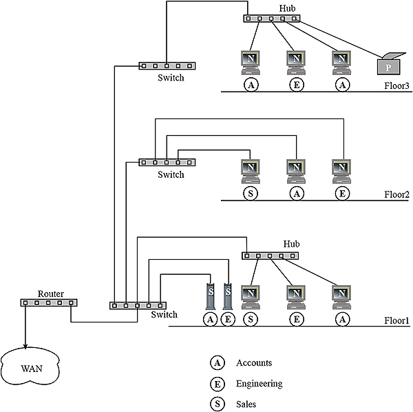
Workgroup distribution within a building
A VLAN logically groups switch ports into workgroups. Since the number of broadcasts and multicasts between the users of a workgroup is likely to be high, a VLAN that includes only members of a given workgroup limits broadcast traffic to the particular workgroup. Thus a VLAN performs like a virtual broadcast domain. Figure 11.4 shows the logically defined VLAN network.

A typical VLAN
11.2 Benefits of a VLAN
VLANs offer a number of advantages over the traditional switched LAN implementation. In networks with a high proportion of broadcast traffic, a VLAN can improve network performance by withholding broadcast messages from unintended destinations. This function could be performed by a router, but the greater amount of processing required for a router increases latency and therefore reduces the performance of the network. A VLAN is simply more efficient.
A VLAN allows a network administrator to allocate a group of users to a virtual broadcast domain, irrespective of their physical location. The only alternative to a VLAN would be to physically move the users. Given that present-day organizations are generally more dynamic, frequent changes in workgroups have also become necessary. This can be achieved by a VLAN without the need of physical relocation every time a change takes place.
A considerable part of the network administration efforts can be attributed to additions, movements and changes; all of which involve reconfiguration of hubs, routers, station addressing and sometimes even re-cabling. It is estimated that roughly 70% or more of administration time is spent on such activities. A VLAN reduces the need for these changes and, with good management tools, all that needs to be done is a simple drag and drop action to change a user from one VLAN to another. The ease of administration, the avoidance of physical relocation and cabling changes, and the elimination of expensive routers to contain broadcast activity keep the costs lower.
Through the ability to contain all transmissions (including broadcasts) within a workgroup, access to sensitive data is limited to members of a specific VLAN. This improves the data security of the network.
11.3 VLAN restrictions
VLANs are not without problems. When resources such as printers have to be shared within a logical group, it may inconvenience printer users physically located far away from the printer.
The present trend is to group different servers in a common server farm with increased physical security, environmental control and fire prevention measures. These servers may have to be accessed by members of more than one VLAN. If it is not possible to assign the server to more than one VLAN, such access is impossible unless the servers are put in a separate VLAN and connected to the other VLANs via a router. This can affect network throughput.
Initial VLAN implementations were by and large proprietary, which hampered inter-operability since VLAN switches for a specific system had to be obtained from one vendor. Standards such as IEEE 802.1Q, supported by multiple vendors, have simplified the implementation of VLANs.
11.4 Basic operation of a VLAN
The switch is the core component of any VLAN implementation, and serves as the infrastructure for frames to or from each node. How VLANs will be grouped is decided by the network administrator, and the switch simply implements this decision. The intelligence required to identify the group to which a frame belongs is provided by the switch, and can be carried out either by packet filtering or by packet identification (also called tagging).
Packet filtering is similar to the technique used by routers. In this method, each packet received by the switch is examined and compared with a filtering table (also called a filtering database). The filtering table, developed for each switch, contains information on user groups based either on port address, MAC address, protocol type or application type. The switch takes appropriate action based on the comparison. Packet filtering thus provides an additional layer of processing for deciding as to how the packet should be handled, which increases the switch latency. It is also necessary for all the switches in the network to maintain and synchronize their filtering tables, which involves administrative overheads.
Packet identification is a relatively new method and consists of placing a unique identifier in the header of each packet before it travels through the switch fabric. The identifier is examined by each switch prior to any broadcast or transmission to other switches, routers or workstations in the network. When a packet exits the switch fabric (routed to the target end station) the switch removes the identifier from the header. Packet identification functions in layer 2 of the OSI model and involves little overhead, apart from the extra four bytes inserted in the Ethernet frame header.
The method of adding an identifier to the frame header for identification purposes is called ‘explicit’ tagging. On the other hand, the method of packet filtering is said to involve ‘implicit’ tagging.
In explicit tagging, the switch needs to know whether the target device is VLAN-aware or not, i.e. whether the target device has the intelligence to interpret the tag information. The identifier is forwarded to a device only if it is VLAN-aware.
11.5 VLAN implementation
The membership of an end user device in a VLAN can be implemented in several ways.
In general, they will fall under one of the following five categories:
- Grouping by switch port
- Grouping by MAC address
- Grouping by Network layer information
- Multicast group
- Higher layer grouping
We will review each of the approaches.
11.5.1 Grouping by switch port
In this method, the membership to a VLAN depends on the switch port to which it is connected. Two types of grouping are possible.
In the first, grouping can be within a single switch, say ports 1, 3, 5 and 7 make up one group and 2, 4, 6 and 8 make up a second group. (Refer to Figure 11.5).

Single switch with ports grouped
In the other method, which will involve more than one switch, a VLAN can include specific ports of different switches. For example: ports 1, 2, 3 and 4 of Switch 1 and ports 1,2, 3 and 4 of Switch 2 form VLAN A and ports 5, 6, 7 and 8 of Switch 1 and ports 5, 6, 7 and 8 of Switch 2 form VLAN B. (Refer to Figure 11.6).

Two switches with ports grouped
The limitation of the method using switch ports to indicate grouping is that whenever a particular user moves to a new physical location involving a different switch/port, the network administrator has to reconfigure the VLAN membership information.
This grouping also works best for nodes that are directly connected to a switch port. If a host is connected to a VLAN switch port through a hub, all the machines connected to the hub have to be members of the same VLAN as one physical segment cannot be assigned to multiple VLANs. However, hubs with a multi-backplane connection feature overcome this limitation to some extent, since each backplane of the hub can be allocated to a particular VLAN.
The switch port grouped implementation works well in an environment where network moves are done in a controlled fashion and where robust VLAN management software is available to configure the ports.
Port based VLANs are set up as follows. The user must configure each port to accept packets (only) from certain other ports. Assume that ports 1, 2 and 3 on a switch have to be set up as members of one VLAN. The switch will then be configured as follows:
- Port 1 egress Port 2, egress Port 2
- Port 2 egress Port 1, egress Port 3
- Port 3 egress Port 1, egress Port 2
11.5.2 Grouping by MAC address
The problem of manual reconfiguration is overcome by grouping different machines based on their MAC addresses. These addresses are machine-specific and are stored on the host’s NIC. This ensures that, whenever a user moves from one switch port to another, the grouping is kept intact and, wherever the move, the user’s VLAN membership is retained without change. This method can therefore be thought of as a user-based VLAN implementation.
This method has some drawbacks. The MAC address-based implementation requires that, initially, each MAC address is assigned to at least one VLAN. This means that to begin with, there will be one large VLAN containing a very large number of users. This may lead to some performance degradation. The problem is overcome by some vendors providing automated tools to create groups based on the initial network configuration. In other words, a MAC address based VLAN is created automatically for each subnet of the LAN.
Serious performance issues can arise if members of different VLANs co-exist in a shared media environment (within a single segment). In the case of large networks the method of communicating the VLAN membership information between different switches to keep them synchronized can cause performance degradation as well.
The use of MAC addresses to identify VLAN membership can also be problematic in a network where a large number of laptop computers are connected to the network by means of docking stations. The NIC, and therefore the MAC address, is a part of the docking station which usually remains on a particular desk. In a situation where the user and the laptop moves around to different desks/docking stations, their MAC address changes when they move to a different desk. This makes tracking groups based on MAC addresses difficult, since reconfiguration is needed whenever a user moves to a different docking station.
11.5.3 Grouping by Network layer information
This method is also referred to as layer 3-based VLAN implementation. Here, grouping is based on information such as the protocol type, or in many cases Network-layer addresses such as the subnet address in IP networks. The switches examine the information regarding the subnet address contained in each packet to decide to which VLAN the user belongs, and makes the forwarding decision on this basis. It should be noted that even though this method uses layer 3 information, it does not constitute routing. This is so because no route calculation is done, frames are usually bridged according to the Spanning Tree Algorithm, and connectivity within any VLAN is seen as a flat bridged topology. See Figure 11.7 for an example of this type of implementation.
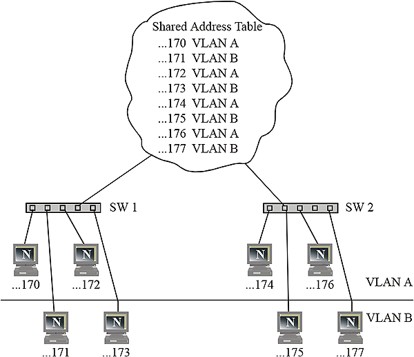
VLAN grouping by Network layer address
Some vendors incorporate varying amounts of intelligence in their switches so that they carry out functions normally associated with layer 3 devices. Some of these layer 3-aware devices have the packet forwarding or routing function built into ASIC chips on the switch, which makes them faster than CPU-based routers. However, the process of examining layer 3 addresses in a packet is definitely slower than looking at MAC addresses in frames since it is located further into the frame. These implementations are therefore slower than those that use layer 2 information.
VLANs using layer 3 information are particularly effective in dealing with networks using TCP/IP. This is not the case with protocols such as IPX or DECnet that do not involve manual configuration at the desktop. In particular, end stations using un-routable protocols such as NetBIOS cannot be differentiated and therefore cannot be included in these VLANs.
11.5.4 VLANs using multicast groups
This represents a different approach to VLANs although the concept of a VLAN as a broadcast domain is still applicable. When an IP packet is sent via multicast, it is sent to an address that is a proxy for a group of IP addresses dynamically defined. Each workstation is given a chance to join this group for a certain period of time by sending an affirmative response to a broadcast. They are, however, members of the multicast group only for a certain period of time. This approach is thus highly flexible and exhibits a high degree of application sensitivity. Such groups can also span routers and therefore WAN connections.
11.5.5 VLANs using higher layer grouping
VLANs implemented in this way are defined on the basis of applications or services or both. For example, FTP applications can belong to one VLAN and TELNET applications to another. Such complex VLAN implementations need a high degree of automation in their configuration and management.
11.6 Interconnection methods
Devices in a VLAN can be connected in different ways depending on whether the device is ‘VLAN-aware’ or ‘VLAN-unaware’. As we saw earlier, a VLAN-aware device can interpret explicitly tagged frames and decide to which VLAN the frame is to be directed.
These connections are referred to as:
- Trunk link
- Access link and
- Hybrid link
We will now discuss these in more detail.
11.6.1 Trunk link
A Trunk link only carries frames in which the tagging information is present. This is normally the case with the links that interconnect switches, but some higher-end NICs are also capable of interpreting the tags. All devices connected to a Trunk link should be ‘VLAN-aware’, including workstations, and all frames on a Trunk link should be explicitly tagged. Figure 11.8 below shows an example.

An example of Trunk links
11.6.2 Access link
An Access link connects a VLAN-unaware device (e.g. a NIC that is incapable of reading the tag information in the frame) to a VLAN-aware switch. VLAN-unaware LAN segments are generally found in legacy LANs. Since VLAN-unaware devices cannot handle explicitly tagged frames, the frames must be implicitly tagged, or in other words, the switch must strip out the tag information before forwarding the frame to the device. Refer to Figure 11.9 for an illustration.

Access links
11.6.3 Hybrid link
When VLAN- unaware end stations are attached to a Trunk link, the resultant link is called a Hybrid link. A Hybrid link is one with VLAN-aware as well as VLAN-unaware devices attached to it. A Hybrid link can therefore carry tagged as well as untagged frames. However, all the frames egressing from a switch to a specific device must be either tagged or untagged, depending on whether that particular device is VLAN-aware or VLAN-unaware. Refer to Figure 11.10 below.

Hybrid links
All three types of links can be present in a single network.
11.7 Filtering table
The filtering table in each switch is a database, which stores the VLAN membership information permitting the switch to decide on how a packet is to be handled. There are essentially two types of entries: static and dynamic.
11.7.1 Static entries
Static entries are created, modified or deleted by the network administrator and are not automatically deleted by ageing, unlike dynamic entries. Static entries can either be filtering entries or registration entries. A filtering entry is made for each port, indicating whether frames to a specific address in a VLAN should be forwarded, discarded or whether they should be subject to a dynamic entry. Static registration entries specify whether frames for a specific VLAN should be explicitly tagged and which ports are members of which VLAN.
11.7.2 Dynamic entries
Dynamic entries are automatically created by the switch and cannot be added or changed by the administrator. Unlike static entries they are automatically removed from the table after a certain time that is decided by the administrator. The learning process takes place by observing the packets sent by a port, identifying the address and VLAN membership. Entries are made accordingly.
The entries can be of the dynamic filtering type, dynamic registration type or group registration type. Dynamic filtration entries specify whether a packet to be sent to a specific address in a particular VLAN should be forwarded or discarded. Dynamic registration entries specify which ports are registered in a specific VLAN. Addition or deletion of entries is done using the Generic Attribute Registration Protocol (GARP) or the VLAN Registration Protocol (GVRP). Group registration entries indicate, for each port, whether frames to be sent to a group MAC address should be filtered or discarded. These entries are added or deleted using Group Multicast Registration Protocol or GMRP. GVRP has another function: communicating information to other VLAN-aware switches. Such switches register and propagate VLAN membership to all the ports that are part of the currently active topology of the VLAN.
11.8 Tagging
Explicit tagging is the process of adding information to the header of a frame (e.g. Ethernet) to indicate the specific VLAN membership for that frame. Unfortunately the ‘standard’ Ethernet/ IEEE 802.3 header does not contain sufficient information to identify VLAN membership; hence the frame had to be modified by the insertion of a ‘tag’ between the two MAC addresses and the Type/Length field. This modified frame is known as an IEEE 802.1Q tagged frame.
The IEEE 802.1p committee defined a standard for packet-based LANs to support layer 2 traffic prioritization in a switched LAN. IEEE 802.1p is part of the larger IEEE VLAN initiative (IEEE 802.1p/Q) that adds more information to the Ethernet header (as shown in Figure 10.11) in order to allow both VLAN operation and traffic prioritization.
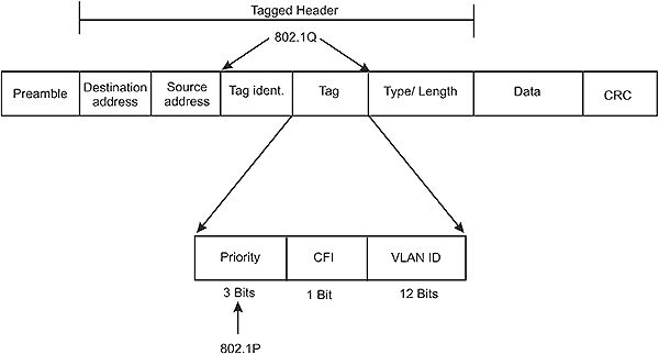
IEEE 802.1p/Q modified Ethernet header
802.1p/Q adds 4 bytes to the Ethernet header. The first field (two bytes) is known as the ‘Tag Identifier’ and assumes the value of 0x8100 for Ethernet. This simply indicates that the frame is tagged and therefore not a standard Ethernet frame.
The following field (2 bytes) contains the tag itself and is subdivided into three fields:
- Priority (3 bits) allows for eight user-defined discrete priority levels from 0 (low) to 7 (high) in order to support different kinds of traffic in terms of their delay-sensitivity. Since IEEE 802.1p/Q operates at layer 2, the Data Link layer, it supports prioritization for all traffic on the VLAN, both IP and non-IP. This introduction of priority levels enables so-called deterministic Ethernet operation where, instead of contending for concurrent access via a switch to a particular end node, a high-priority source node can pass a frame almost immediately to a destination node, and without risk of collisions.
- TR (1 bit), also referred to as the Canonical Format Indicator (CFI), indicates whether the VLAN number in the following field is written with its MSB on the left or on the right.
- VLAN ID (12 bits) governs the VLAN membership, through a user-defined number between 1 and 4095
12.1 Introduction
Large, multi-site businesses have always emphasized centralized information systems as an important objective in their IT policy framework. With the explosion of communication technologies, many of them have achieved this objective by establishing WANs via leased communication channels. This has made possible the access of corporate information by all branch offices in a continuous and almost real-time manner, which, in turn, led to better decision-making. WANs are, however, expensive to set up and maintain, given the high cost of leased lines. They are therefore beyond the reach of many small and medium businesses.
Another aspect of corporate networks is remote access. Employees who work from home or are constantly on the move often have to access their corporate LAN to access their e-mail and to obtain other pertinent information needed for their business interactions. This type of communication was traditionally done via dial-up connections using modems and public telephone networks, often over long distances or sometimes even through international circuits. This is more expensive and less secure compared with dedicated leased circuits. Figure 12.1 shows a typical corporate network with inter-site WAN connectivity and remote user access.

A typical corporate network
There has been a paradigm shift in the approach to corporate networking since the advent of the Internet as a business communication medium. Given the ubiquitous nature and low access cost of the Internet, other more attractive networking solutions have started arriving in the IT marketplace. Virtual Private Network (VPN) technology has started replacing conventional leased circuit-based WANs. In this chapter we will explore the fundamental concepts of this technology and see how it is helping businesses to redefine their IT approach while simultaneously effecting considerable savings in their communication budgets.
The Internet has affected computing in more than one way. Information dissemination within the organization through Intranets uses the same standards as the Internet. Web-enabled applications use multi-tier architectures for database access and are deployed both within the corporation and for external customers. This has enabled the adoption of a unified application architecture for employees, business partners and the public domain realized by the Intranet, Extranet and Internet respectively. A VPN is the infrastructure that makes such deployment possible in a cost-effective manner. A typical view of an Enterprise network using VPN technology is shown in Figure 12.2.

A typical Enterprise network using VPN technology
12.2 What is a VPN?
A VPN is basically a corporate network built around the communication infrastructure of the Internet instead of leased lines or RAS using direct dial-in. Since the Internet is a public medium where the traffic is prone to interception or modification, security issues play an important role in the implementation of a VPN. A VPN is, however, a highly cost effective proposition as dedicated lines are required only to connect the corporate network to an ISP (usually located within the same city). Remote users of a VPN also connect to the network through the Internet using local dialup access numbers (Points of Presence) of the ISP. This offers a very high degree of availability and Quality of Service (QoS) as opposed to long distance dialing. The actual savings will depend on many factors including the geographical spread of enterprise branch locations, the number of remote users, locations from where remote access is generally made and the average time of use by the remote users. It has been reported that a saving of up to 50% is possible by changing over from a conventional WAN to a VPN. Capital expenditure payback periods for VPN implementation can be as low as four months.
12.3 Types of VPN
VPN solutions are essentially of three distinct types.
- Inter-site or inter-LAN VPNs. These provide connectivity among multi-user branch office LANs and the central enterprise LAN through the Internet, replacing more expensive solutions based on leased lines (few-to-few connectivity).
- Remote access VPNs. These provide many-to-few of connectivity for mobile remote users and telecommuters to a corporate LAN through the Internet.
- Extranets are used by business partners of the corporation such as vendors, dealers etc. through the Internet for electronic commerce, product information, business support systems, and other aspects of day to day business needs.
While all three of these types of connectivity are essential from the enterprise viewpoint, most of the savings result from Remote Access VPN. This is because:
- The cost of remote access and the number of employees who travel and need to connect using long distance dial-up are showing an increasing trend.
- A dial-up Internet connection offers good bandwidth and is therefore becoming acceptable to more users, particularly those using applications based on client-server technology and multi-tier architectures that conserve bandwidth.
- A local dialup connection using a reliable ISP offers a very high degree of availability and QoS level compared to direct dial-up through long distance lines.
12.4 Requirements for designing a VPN
Any enterprise planning to implement a VPN system must carefully evaluate the various issues of importance. A 5-tier model proposed by the Gartner Group summarizes these issues and can be a starting point. See Figure 12.3 below.

A 5-tier model for VPN implementation
The five tiers are security, scalability, manageability, simplicity and quality of service. Security is a factor decided by the corporate policy. Scalability, manageability and simplicity are functional requirements and will depend on present and perceived future needs, particularly the issue of scalability. QoS will be primarily dependent on the ISP whose infrastructure will be used for the VPN. The task of implementation can thus be divided into:
- Defining overall policies and user privileges
- Defining functional requirements
- Infrastructure planning and arriving at an integrated VPN solution
We will discuss these aspects in further detail in the following sections.
12.5 Defining policies
In any network, certain policy guidelines are established by the IT department to ensure appropriate and optimal use of network resources. Most enterprises would have developed such guidelines even before considering a VPN. The main issues to be addressed are:
- Security policies
- Access rights
- Cost thresholds
- Class-of-service usage
The access rights and cost threshold issues are quite straightforward and are defined as a part of organizational structure of the enterprise. Class of Service issues such as bandwidth commitments to different functional groups require a more thorough evaluation. In addition, such facilities can only be realized using specialized VPN implementations.
It is, however, the issues concerning security that normally need very careful consideration. We will go through this aspect in detail later in this chapter.
12.6 Functional requirements
While planning to implement a VPN, it is necessary to understand the needs and expectations of users as well as network administrators in order to choose a suitable system. While network administrators will look for scalability and manageability, the users will need simplicity of usage. The VPN should satisfy all these three basic parameters namely scalability, manageability and simplicity.
12.6.1 Scalability
It is an extremely difficult task to decide the scalability of VPN systems. Scalability is determined by the growth of user population and growth of usage in terms of both time and bandwidth. Growth itself is driven by the following factors.
- Lower cost of connectivity; as cost falls, usage increases.
- Higher speeds of connectivity that makes it possible for more applications to run satisfactorily and enhances usage.
- More capable and portable hardware at lower cost
- Wider applications of the Internet
In short, continued improvement in connectivity at a lower cost will significantly boost the use of VPN as more employees will tend to work away from the office, in increasing numbers and for increased hours.
User population is a critical design element. If there are 600 remote users in a corporation, each user will require a dedicated channel (called a Tunnel in VPN terminology) to access the central host. Since not all users are expected to connect at the same time, it is usual to have 200 to 300 tunnels for 600 users (over-subscription by a ratio of 2:1 to 3:1). However, as the time of usage increases, the ratio must become lower, if one is to obtain a connection on demand. Increase in user population also puts increasing demands on Internet connectivity resources, such as bandwidth of the Internet connectivity at the central site as well as its routers, firewalls, authentication systems and server hardware. All these must scale upwards to keep up with the increased demand. Any inadequacy in these resources will increase the response time and will result in poor network performance and user dissatisfaction.
It is advisable to plan for a little excess capacity in the beginning so that capacity constraints do not become an issue immediately after the initial implementation.
- Link performance is another aspect that needs attention. The performance depends primarily on latency and packet loss.
- Latency is the time required for a packet to traverse the Internet. It is a function of router hops between sender and receiver; the more hops, the higher is the latency. The end station processing bottleneck is another factor in increasing latency. Increased latency often affects interactive applications to a considerable extent. The TCP protocol has an inherent problem due to the type of window management used in this protocol. Most VPN products use TCP to ensure correct delivery of packets and are thus vulnerable to this problem.
- Packet loss causes a much higher degree of performance degradation than latency. This is because the packet loss needs to be identified before a request for re-transmission is made and re-transmission occurs. TCP could discard the whole window (all packets transmitted between successive acknowledgements) unless selective acknowledgement is supported. This can cause a considerable reduction in link throughput in the case of packet loss. A very small window size (such as used by the PPTP protocol, which has a window size of three packets) ensures less degradation if a packet is lost. At the same time, it results in more idle time since a latency period is added once for each set of 3 packets. A large window size results in faster transmission but causes higher recovery time in case of a packet loss. A balance therefore has to be struck by optimizing the window size. A possible solution is to have a variable window size depending upon the degree of packet loss (e.g., decrease window size if less packet loss is noticed). Selective re-transmission of lost packets alone can improve performance. Packet loss can slow down certain types of encryption and compression algorithms, as these techniques require orderly packet delivery. Some VPN systems perform compression after encryption. Since encrypted data is very random-looking, compression of encrypted data is not very effective. Compression prior to encryption yields better results and increases network throughput.
- Tunnel server architecture is another aspect that determines the scalability. The tunnel server is the device that serves as the point of access of a remote user. Efficient utilization of the entire capacity of the Internet connection bandwidth depends on the tunnel server. If link bandwidth is increased or multiple links are added, the tunnel server must scale up to use the increased bandwidth available to it. It is a normal practice to operate more than one tunnel server in a cluster to provide redundancy as well as increased traffic handling capacity. The system should incorporate load-balancing measures for maximizing the throughput and link performance.
There are two ways in which a server cluster can be used. One method (Figure 12.4) is to have a pure cluster with a single Internet access point. The other method (Figure 12.5) is to have parallel servers, each with its own Internet connection.

Pure cluster of tunnel servers

Parallel tunnel server cluster
An alternative to the clustering of multiple servers is to have distributed servers by placing the tunnel servers closer to different application servers. While the type of automated load sharing as done in clustered servers is not possible, the architecture itself has the effect of balancing the load and provides adequate redundancy.
A VPN system should have quantifiable scalability attributes and should have effective data compression. It should also provide for protocol extensions such as variable window size and selective packet re-transmission. Such capabilities will ensure better performance.
12.6.2 Manageability
The next important functional requirement from the administrator’s point of view is end-to-end manageability from a single control point. Manageability should include information on user population, login status, system status, traffic loading, managing of remote user desktops, Internet connection management, etc. We will review some of the important requirements.
- User management must provide for a centralized facility that lists all VPN clients, their access privileges and authentication data. It should allow easy addition, moves and changes of users and their profiles. It should be simple and intuitive to use. This facility should also extend to the client desktop and should permit features such as auto dialling of the local POP of an ISP and reporting of connection status and problems to the central site.
- Connection management ensures that all connection policies, cost control and security procedures are performed properly at the remote desktop. The features should include:
- Auto dialing to the least expensive POP from any remote point in the world that matches the speed of the user.
- Terminating and reconnecting to an alternate route if throughput falls below a threshold value
- Monitoring user login time and terminating or preventing connection if pre-set limits are exceeded.
- Management of availability should be a feature of the VPN system, and should permit centralized monitoring of network health. Client VPN implementation should be able to automatically correct configuration problems and automatically download POP information changes. These measures will ensure that the central management is not swamped with too many tasks and create a management bottleneck. The availability management tools should also monitor connection performance so that a breach of committed service levels of the ISP can be detected early and corrective action taken.
- Distributed Management Architecture is another important requirement. Managing a large VPN from a central console is often impractical as it may require more than one person to handle management tasks. In addition to this, management from remote machines should be possible, as administrators cannot be present in the office at all times. Thus, while the management server can be centralized, the management application itself must be a separate component that can run on a number of machines and allow distributed management. In some cases, part of the management can be performed at the ISP end by the ISP, so that troubleshooting of the network segments within the ISP’s control becomes easier. Figure 12.6 shows an implementation of a Distributed Management Architecture.

VPN distributed management architecture
12.6.3 Simplicity
A VPN system is essentially quite simple in concept. However, for a user who is not a systems specialist, the procedures of access and connectivity can be daunting. By designing a simple and easy-to-use interface, these complexities can be hidden from the user and all that he/she will see is a consistent screen irrespective of the method of connectivity. In addition, all ISP/route/cost decisions should be automated. Access telephone numbers and dial-up codes at remote locations should be based on table look-up and should be transparent to the user. The user should not be required to remember multiple passwords irrespective of the ISP and location of POP.
The user interface should have the necessary intelligence to gather information on connectivity performance, QoS issues such as difficulty in access, lower than committed speeds, etc. and report them to the centralized VPN management system for analysis and corrections.
Dynamic fault recovery is another prerequisite. Rather than just detecting a fault and reporting it to the user, the client application should resolve the problem by itself to the extent that this is feasible. It should also automatically download and update drivers as well as look-up tables containing access information whenever there are changes to these data or files. Automatic reconnection in case of sudden disconnection is another desirable feature.
A simple and automated user interface will result in fewer help desk calls and result in better user satisfaction and cost savings.
12.6.4 Network infrastructure
In almost all cases where a VPN implementation is planned, an existing network with both Internet access and RAS is likely to be in operation. The VPN implementation should integrate properly into this legacy environment. Figure 12.7 shows such a typical legacy environment.

Existing legacy network environment
Any VPN must be designed to complement the existing equipment. For example, the Internet router will still be needed for Internet access. Usually such routers also act as layer 3 firewalls, a function that VPN equipment do not provide. Similarly, corporate LAN routers that enable multi-protocol routing should also be retained, as VPNs do not have LAN routing capability. The firewall hardware has to be retained as well because a VPN’s basic access control is, by itself, not an adequate protection measure.
Figure 12.8 shows the possible ways in which the tunnel server can be placed in an existing corporate network.

Adding VPN hardware in an existing LAN
In the arrangement shown in Figure 12.8A, the inbound VPN traffic is also made to go through the firewall before accessing the tunnel server. This may require the firewall to be upgraded as VPN traffic increases. In figure 12.8B, the VPN traffic is handled directly by the tunnel server whereas non-VPN traffic is sent through the firewall. This arrangement is more scalable.
12.7 Security
Security is a vital concern in the planning of a VPN. As the Internet is a notoriously uncontrolled and public medium, any traffic through the Internet poses many security risks. These are addressed using the following protective measures.
- Authentication
- Encryption
- Use of tunneling protocols
12.7.1 Authentication
Authentication identifies a user to the system, the most common method being the use of a password. Passwords must follow a clear policy. Users should take care not to make the password too easy to guess and not to share the password with others. The system may enforce a minimum length of passwords, use of one or more special characters in the password; force periodic changes of password and disallow password repetition. If proper password policies are not adopted and enforced, the security of any network can be seriously compromised. The authentication system compares the password that the user provides with the password database in the server and, if they match, permits access.
Some of the protocols used for VPNs are based on PPP, which was traditionally used for RAS access with authentication by the Password Authentication Protocol (PAP).
Sending the password in clear text over a public network is risky, as passwords can be revealed to those who eavesdrop on the network. A variety of challenge-response protocols is therefore used. One example is the Challenge Handshake Authentication Protocol or CHAP. In this system, the authentication of users is done by the following steps.
- A database of users and passwords is maintained by the network administrator.
- Request for login is received by the authentication server
- The server issues a random challenge
- The client calculates a hash based on the random challenge and the password using a one-way function and sends the hash (not the password) over the network.
- The server computes the password by using the same one-way function and the random challenge. If this password matches the password in the database for that user, authentication is successful.
It is possible to use stronger authentication models, which require that, in addition to the password, the user also has to identify himself through some other means. This may be a hardware-based token card or identification based on scanning of a thumbprint or iris scan. This combines something that the user knows (password), with something that he has (a card or thumbprint) as means of identification. This is, however, subject to the support by the VPN protocol being used.
Many VPNs support SecurID by Security Dynamics, a token card that combines secret key encryption with a one-time password. The password is automatically generated by encrypting a timestamp with a secret key. This one-time password will be valid for a short interval, usually 30 to 60 seconds.
Digital certificates are also becoming more prevalent as an authentication mechanism for VPNs. A digital certificate (based on the X.509 standard) is an electronic document that is issued to an individual by a ‘Certificate Authority’ (CA) that can vouch for an individual’s identity. It essentially binds the identity of an individual to a public key. A digital certificate will contain a public key, information specific to the user (name, company, etc.), information specific to the issuer, a validity period and additional management information. This information will be used to create a message digest, which is encrypted with the CA’s private key to ‘sign’ the certificate.
By using the digital signature verification procedure described above, participants in a conversation can mutually authenticate each other. Although this process sounds simple, it involves a complex system of key generation, certification, revocation and management, all part of a Public Key Infrastructure (PKI). A PKI is a broad set of technologies that are used to manage public keys, private keys and certificates. The deployment of a PKI solution should be done with due care as there are major issues such as scalability and interoperability.
Manual authentication provides a means for authenticating network devices including firewalls, gateways and desktop clients by the CA. The process allows the registration authority to control the certificate lifecycle including approval and renewal of certificates. The sequence goes something like this:
- The network/firewall administrator sends an email to all remote users that they need to download a copy of the required software from an Intranet location.
- The user downloads and installs the software and completes the certificate request form.
- The administrator receives an email that User A has requested a certificate.
- The administrator connects securely to the CA’s on-site control center, which approves or rejects the request for a certificate. If the certificate is approved, the control center will send an email telling the user to pick up his certificate.
- After the certificate has been approved, the administrator downloads the current directory list (LDIF file) and either imports it into the user database or an LDAP (Lightweight Directory Access Protocol). The user picks up their certificate with their browser.
- The user can now securely connect to the corporate network from anywhere on the Internet.
- When the user tries to authenticate with the firewall, the firewall will compare the certificate against the current Certificate Revocation List (CRL). If the certificate is not on the CRL and the user is on the valid access control list, then a secure connection is created.
For remote users, other methods such as pass code authentication and automatic authentication can be used to obtain the digital certificate.
Increasingly, disparate remote access and VPN systems are managed by a central user account and policy database. This requires a schema that can be used irrespective of the VPN vendor and the authentication method that the vendor deploys. The Remote Access Dial-In User Services (RADIUS) protocol is one such initiative for unifying devices from multiple vendors into one authentication scheme. Any VPN or RAS device that supports RADIUS can authenticate against a central RADIUS server which not only defines the user names and passwords, but can also maintain remote user policies such as IP addresses, allowed length of call and number of concurrent logins.
| Step 1 | Client requests a connection |
| Step 2 | Management server sends random challenge to client |
| Step 3 | Client calculates a hash based on the challenge and its password and returns the hash to the Management server |
| Step 4 | Management server sends challenge and hash to RADIUS server in an Access-Request message |
| Step 5 | RADIUS server calculates the hash and compares it to the client’s hash, if they match then it responds with an Access-Accept message |
| Step 6 | Management server grants connection to client |
Figure 12.9 shows a typical RADIUS scheme in operation.

Radius server based authentication
Microsoft and Novell have released RADIUS support for their respective network operating systems in order to provide remote user access management.
Authentication does not stop with user identification. The packets that go through the Internet are vulnerable to several threats such as spoofing, session hijacking, sniffing, and man-in-the-middle attacks. It is therefore necessary to examine the packets and make sure that they originate from the purported sender and not someone masquerading as the sender. The checks include:
- Data Origin Authentication which ensures that each datagram originated from the claimed sender
- Data integrity checks to verify that the contents of the datagram were not changed in transit, either deliberately or due to errors
- Replay protection to ensure that an attacker can not intercept a datagram and play it back at some later time
We will discuss these aspects further when we review VPN protocols.
12.7.2 Encryption
Encryption refers to the alteration of data using a key (which is a fixed length string of bits) so that the data is meaningless to anyone intercepting the message unless he has the key. The reverse process of getting the data back from the encrypted form is called decryption and is done by the receiver using the same key. It is essential that both sender and receiver share the key. This method where a shared key is used by both sender and receiver is called symmetrical encryption or Private Key encryption. It is possible to attack an encrypted message using ‘brute force’ method through an automated process of trying out all possible key combinations. Therefore the longer the key length, the more difficult it is to break. A 128-bit string will take thousands of years of computational time to break by ‘brute force’ methods and is therefore considered safe.
The other method that is increasingly used requires a set of two keys, a public key and a private key. Diffie-Hellman (DH) and Rivest-Shamir-Adleman (RSA) are two of the popular algorithms in common use.
In this method every user has a set of two keys, a public key that is revealed to anyone who wishes to contact him and a private key that is not shared with anyone. When a message is sent by A to B it is encrypted by using the public key of B. Once it is received by B, he decrypts it using his private key. Decryption is not possible without knowing this key. Refer to Figure 12.10, which illustrates this operation.

Use of Public and Private Key
In addition to user authentication, Certification Authorities (CAs) also provide digital certificates containing the Public key. An enterprise can implement its own certification using Certification Servers, or use third party services such as Verisign for issue and sharing of their public key. This process of managing public keys is known as the Public Key Infrastructure (PKI).
12.7.3 VPN protocols
VPN works over the Internet but it is possible that the communication protocol used in the corporate LAN is different and not the TCP/IP protocol used on the Internet. It may be IPX (Novell) or NetBEUI (Microsoft). If these protocols have to work between a remote client and the central server, there must be a mechanism to encapsulate their protocol packets within IP packets for transportation and reassemble them into the native LAN protocol at the receiving end. This process is called encapsulation.
In addition, the internal network addresses should be preferably hidden from public view, particularly when TCP/IP is used as the LAN protocol, by encrypting the address along with the data. This way, the packet travels from sender to receiver through the Internet in a secure tunnel and comes out at the other end to be processed further. Thus, a VPN can be implemented in such a way that no change is required in the LAN or application architecture.
A tunnel is required for each remote user and the tunnel server should be capable of providing the required number of tunnels on the basis of simultaneous remote connections at any given point in time.
Four protocols are generally used in VPNs. They are the Point-to-Point Tunneling Protocol (PPTP), Layer-2 Forwarding protocol (L2F), Layer 2 Tunneling Protocol (L2TP), and the IP Security Protocol (IPSec).
PPTP, L2F and L2TP are aimed at remote users connecting through dial-up access. IPSec is aimed at LAN-to-LAN VPNs.
PPTP
PPTP is derived from the popular Point-to-Point Protocol (PPP) used for remote access to the Internet. PPTP has added the functionality of tunneling through the Internet to a destination site. The encapsulation of PPP packets is done using a modified Generic Routing Encapsulation (GRE) protocol. PPTP can be used for any protocol including IP, IPX and NETBEUI. It has, however, some limitations such as its inability to support stronger encryption and token based user authentication.
With PPTP in a tunneling implementation, the dial-in user has the ability to choose the PPTP tunnel destination after the initial PPP negotiation. This is important if the tunnel destination will change frequently, and no modifications are needed by mechanics in the transit path. It is also a significant advantage that the PPTP tunnels are transparent to the service provider, and no advance configuration is required between the NAS operator and the overlay dial access VPN (VPDN). In such a case, the service provider does not house the PPTP server, and simply passes the PPTP traffic along with the same processing and forwarding policies as all other IP traffic.
In fact, this could be considered a benefit, since configuration and support of a tunneling mechanism within the service provider network need not be managed by the service provider, and the PPTP tunnel can transparently span multiple service providers without any explicit configuration.
The other advantage is that the subscriber does not have to pay a higher subscription fee for a VPN service. The situation changes dramatically if the service provider houses the PPTP servers, or if the subscriber resides within a sub-network in which the parent organization wants the network to make the decision concerning where tunnels are terminated. The major part of PPTP-based VPDN user base is one of a roaming client type, where the clients of the VPDN use a local connection to the public Internet data network, and then overlay a private data tunnel from the client’s system to the desired remote service point.
L2F
L2F was developed in the early stages of VPN and also uses tunneling. Like PPTP, L2F also uses PPP for authentication but also supports Terminal Access Controller Access Control System (TACACS+) and RADIUS. Unlike PPTP, L2F tunneling is not dependent on IP but can work directly with other media such as ATM and Frame Relay. In addition, L2F allows tunnels to support more than one connection. This protocol has now given way to the later L2TP.
L2TP
L2TP, designed by the IETF working group to succeed PPTP and L2F, uses PPP to provide dial-up access that can be tunneled to a corporate site through the Internet, but defines its own tunneling protocol. Like L2F, it can also handle multiple media and offers support to RADIUS authentication. L2TP can support multiple, simultaneous tunnels for each user.
With L2TP in a ‘compulsory’ tunneling implementation, the service provider controls where the PPP session is terminated. This can be extremely important in situations where the service provider to whom the subscriber is actually dialing into (let’s call this the ‘modem pool provider’ network) must transparently hand off the subscriber’s PPP session to another network (let’s call this network the ‘content provider’).
To the subscriber, it appears as though he is directly attached to the content provider’s network, when in fact he has been passed transparently through the modem pool provider’s network to the service to which he is subscribed. Very large content providers may outsource the provisioning and maintenance of thousands of modem ports to a third-party provider, who in turn agrees to pass the subscriber’s traffic back to the content provider. This is generally called ‘wholesale dial.’ The major motivation for such L2TP-based wholesale dial lies in the typical architecture of the PSTN (Public Switched Telephone) Network.
The PSTN network is typically constructed in a hierarchical fashion, where a local PSTN exchange directly connects a set of PSTN subscribers, which is in turn connected via a trunk bearer to a central office or metropolitan exchange, which may be connected to a larger regional office or major exchange. A very efficient means of terminating large volumes of data PSTN calls is to use a single common call termination point within the local or central exchange to terminate all local data PSTN calls, and then hand the call data over to a client service provider using high volume data transmission services. This cost efficiencies that can result from this architecture form a large part of the motivation for such L2TP-based VPDNs, so a broad characterization of the demand for this style of VPDN can be characterized as a wholesale/retail dial access structure. Another perspective is to view this approach as ‘static’ VPDN access.
Although L2TP provides cost-effective access, multi-protocol transport, and remote LAN access, it does not provide cryptographically robust security features. For example,
- Authentication is provided only for the identity of tunnel end points, but not for each individual packet that flows inside the tunnel.
- L2TP itself provides no facility to encrypt user data traffic.
- While the payload of the PPP packets can be encrypted, the PPP protocol suite does not provide mechanisms for automatic key generation or for automatic key refresh.
Some of these issued can be addressed by the use of the IPSec protocol.
IPSec
IPSec is the de facto standard for VPNs and is a set of authentication and encryption protocols, developed by the IETF and designed to address the inherent lack of security for IP-based networks. It is designed to address data confidentiality, integrity, authentication and key management, in addition to tunneling.
IPSec, which was originally meant for the next generation of IP (IPv6), can now be used with IPv4 as well. The issue of exchange and management of keys used to encrypt session data is done using the ISAKMP/Oakley scheme, now called Internet Key Exchange (IKE). IPSec allows authentication or encryption of an IP packet, or both. There are two different methods of using IPSec. These are the Transport mode in which only the Transport layer segment of an IP packet is authenticated or encrypted, or the Tunnel mode, where the entire IP packet is authenticated or encrypted.
IPSec uses Diffie-Hellman key exchanges for delivering secret (private) keys on a public network. It uses public-key cryptography for signing Diffie-Hellman exchanges so that the identity of the parties is hidden from the ‘man-in-the-middle’. It encrypts data using the Advanced Encryption standard (AES). It uses the HMAC, MD5 and SHA keyed hash algorithms for packet authentication and validates public keys using Digital Certificates.
However, IPSec is only suitable for networks that use the IP environment and can only handle IP packets. Multi-protocol environments will still need to use PPTP or L2TP.
The IPSec protocol suite typically works on the edges of a security domain. Basically, IPSec encapsulates a packet by wrapping another packet around it. It then encrypts the entire packet. This encrypted stream of traffic forms a secure tunnel across an otherwise unsecured network.
The principal IPSec protocols are:
- IP Authentication Header (AH), which provides data origin authentication, data integrity and replay protection
- IP Encapsulating Security Payload (ESP), which provides data confidentiality, data origin authentication, data integrity, and replay protection
- Internet Security Association and Key Management Protocol (ISAKMP), which provides a method for automatically setting up security associations and managing their cryptographic keys.
We will discuss these in the following paragraphs.
Authentication Header
The IP Authentication Header provides connectionless (that is, per-packet) integrity and data origin authentication for IP datagrams, and offers protection against replay. Data integrity is assured by the checksumↃ generated by a message authentication code (for example, MD5); data origin authentication is assured by including a secret shared key in the data to be authenticated and replay protection is provided by use of a sequence number field within the AH Header. In the IPSec vocabulary, these three distinct functions are lumped together and simply referred to as ‘authentication’.
The algorithms used by the AH protocol are known as Hashed Message Authentication Codes (HMAC). HMAC applies a conventional keyed message authentication code twice in succession, as shown in schematic form in Figure 12.11, first to a secret key and the data, and then to the secret key and the output of the first round. Since the underlying message authentication code in Figure 12.11 is MD5, this algorithm is referred to as HMAC-MD5. The AH protocol also supports the use of HMAC-SHA in which the Secure Hash Algorithm (SHA) is used as the base message authentication code instead of MD5.

Hashed message authentication code
AH protects the entire contents of an IP datagram except for certain fields in the IP header (called mutable fields) ↃↃthat could normally be modified while the datagram is in transit.
For the purpose of calculating an integrity check value, the mutable fields are treated as if they contained all zeros. The integrity check value is carried in the AH header Ↄfield shown in Figure 12.12. AH can be applied in either of two modes: transport mode or tunnel mode. Figure 12.12 shows how the AH protocol operates on an original IP datagram in each of these two modes.

AH in Tunnel and Transport mode
In transport mode, the original datagram’s IP header is the outermost IP header, followed by the AH header, and then the payload of the original IP datagram. The entire original datagram, as well as the AH Header itself, is authenticated and any change to any field (except for the mutable fields) can be detected. All information in the datagram is in clear text form, and is therefore subject to eavesdropping while in transit.
In tunnel mode, a new IP header is generated for use as the outer IP header of the resultant datagram. The source and destination addresses of the new header will generally differ from those used in the original header. The new header is then followed by the AH header, and then by the original datagram in its entirety, including both IP header and the original payload. The entire datagram (new IP Header, AH Header, IP Header, and IP payload) is protected by the AH protocol. Any change to any field (except the mutable fields) in the tunnel mode datagram can be detected.
ESP
The Encapsulating Security Payload provides data confidentiality (encryption), connectionless (per-packet) integrity, data origin authentication, and protection against replay. ESP always provides data confidentiality, and can optionally provide data origin authentication, data integrity checking, and replay protection. When comparing ESP to AH, it is clear that only ESP provides encryption, while either can provide authentication, integrity checking, and replay protection. ESP’s encryption uses a symmetric shared key: That is, a shared key is used by both parties for encrypting and decrypting the data that is exchanged between them.
When ESP is used to provide authentication functions, it uses the same HMAC algorithms (HMAC-MD5 or HMAC-SHA) as in the case of the AH protocol. However, the coverage is different, as shown in Figure 12.13.

ESP in Tunnel and Transport mode
In transport mode, ESP authentication functions protect only the original IP payload, but not the original IP header unlike in AH. ↃIn tunnel mode, ESP authentication protects the original IP header and the IP payload, but not the new IP header.
ESP can be applied in either of two modes: Transport mode or Tunnel mode. ↃIn Transport mode, the datagram’s original IP header is retained. Only the payload of the original IP datagram and the ESP trailer are encrypted. Note that the IP header itself is neither authenticated nor encrypted. Hence, the addressing information in the outer header is visible to an attacker while the datagram is in transit. In tunnel mode, a new IP header is generated. The entire original IP datagram (both IP header and IP payload) and the ESP trailer are encrypted. Because the original IP header is encrypted, its contents are not visible to an attacker while it is in transit. A common use of ESP tunnel mode is thus to hide internal address information while a datagram is tunneledↃ between two firewalls.
IKE
In any IPSec protocol based communication, a Security Association (SA) contains all the relevant information that communicating systems need in order to execute the IPSec protocols, such as AH or ESP. For example, an SA will identify the cryptographic algorithm to be used, the keying information, the identities of the participating parties, etc. ISAKMP defines a standardized framework to support negotiation of SAs, initial generation of all cryptographic keys, and subsequent refresh of these keys. Oakley is the mandatory key management protocol that is required to be used within the IKE framework. IKE supports automated negotiation of security associations, and automated generation and refresh of cryptographic keys. The ability to perform these functions with little or no manual configuration of machines is critical as a VPN grows in size. The secure exchange of keys is the most critical factor in establishing a secure communications environment—no matter how strong the authentication and encryption are, they are worthless if a key is compromised. Since the IKE procedures deal with initializing the keys, they must be capable of running over links where no security can be assumed to exist—that is, they are used to bootstrap Ↄthe IPSec protocols. Hence, the IKE protocols use the most complex and processor-intensive operations in the IPSec protocol suite.
IKE requires that all information exchanges must be both encrypted and authenticated: no one can eavesdrop on the keying material, and the keying material will be exchanged only amongst authenticated parties. In addition, the IKE methods have been designed with the explicit goals of providing protection against several well-known exposures:
- Denial of Service. The messages are constructed with unique cookies that can be used to quickly identify and reject invalid messages without the need to execute processor-intensive cryptographic operations
- ‘Man-in-the-Middle’ protection is provided against the common attacks such as deletion of messages, modification of messages, reflecting messages back to the sender, replaying of old messages, and redirection of messages to unintended recipients
- Perfect Forward Secrecy. There is no risk of a compromise due to knowledge of any past keys as they bear no useful clues for breaking any other key, whether it occurred before or after the compromised key. Each refreshed key is derived without any dependence on the previously used keys.
Outcome
After studying this chapter you should be able to describe, in basic terms, the concept of Voice over IP (VoIP) with reference to the following:
The protocols supporting VoIP, in particular Multicast IP, RTP, RTCP, RSVP and RTSP.
The H.323 standard, with reference to:
- The H.323 hardware, viz. Terminals, Gateways, Gatekeepers and MCUs.
- The H.323 protocols, viz. H.225 and H.245.
- The various related audio and video codecs.
13.1 Introduction
This chapter deals with the convergence of conventional PSTN networks and IP based internetworks, in particular the Internet. As a result of this convergence, Voice over IP is making major inroads into the telecommunications industry. This chapter will introduce the ITU-T H.232 standard for multimedia (audio, video and data) transmission.
H.323 requires IP as a Network layer protocol and TCP/UDP as Transport layer protocols. These protocols have already been covered in chapters 6 and 7.
The major advantage of VoIP over conventional PSTN usage is cost. It is not uncommon for a large company to recover the installation cost of VoIP equipment in less than a year. The following are a couple of implementations.
- Interoffice networking. Instead of having separate voice and data networks within the building, employees can use their telephones as well as their computers on one line.
- Outbound calls. By using the company’s existing infrastructure (X.25, ATM, Frame Relay etc) for outbound calls, the company can save on line rental by reducing the number of outgoing trunk lines.
- Internet surfing at home. Broadband users can not only make phone calls on their PSTN line while on the Internet, but can also make VoIP calls over the internet at a reduced cost. Skype and Voise are good examples of this technology. Even dial-up users with only one line can answer incoming calls on their PCs while surfing the Internet by means of the appropriate software supplied by their phone utility.
- Long distance outbound calls. Companies making a large percentage of their long-distance outbound calls to a few area codes (typical of countries like South Africa and Australia) can install H.323 Gateways in those areas, with the result that for billing purposes these calls become local calls.
- Inbound Customer (1-800) charges. The same philosophy applies. By placing H.323 Gateways in areas where most inbound calls originate, those inbound calls appear as local calls to the callers. The only cost to the vendor is the Gateway installation.
13.2 Protocols

VoIP protocols
13.2.1 Multicast IP
In most applications IP is used for unicasting, i.e. messages are delivered on a one-to-one basis. IP Multicasting delivers data on a one-to-many basis simultaneously. To support multicasting, the end stations must support the Internet Group Management Protocol, IGMP (RFC 1112), which enables multicast routers to determine which end stations on their attached subnets are members of multicast groups. IPv4 class D addresses ranging from 224.0.0.0 to 239.255.255.255 were originally reserved for multicasting.
In order to deliver the multicast datagrams, the routers involved have to use modified routing protocols, such as Distance Vector Multicast Routing Protocol (DVMRP) and Multicast Extensions to OSPF (MOSPF).
13.2.2 RTP
IP provides a connectionless (unreliable) service between two hosts. It does not confirm delivery at all, and cannot deliver packets on a real-time basis. It is up to a protocol at a higher level to determine whether the packets have arrived at their destination at all. There is an added complication in the case of real-time data such as voice and video, which require a deterministic type of delivery.
This problem is addressed by the real-time transport protocol (RTP), an Application layer protocol described in RFC1889, which provides end-to-end delivery services such as sequence numbering and stamping for data with real-time characteristics such as interactive audio and video. User applications typically run RTP on top of UDP to make use of its multiplexing and checksum services, but RTP may also be used with other suitable underlying network or transport protocols.
RTP itself does not provide any mechanism to ensure timely delivery nor does it provide other quality-of-service guarantees, but it relies on lower-layer services to do so. It does not guarantee delivery or prevent out-of-order delivery, nor does it assume that the underlying network is reliable or that packets are delivered in the correct sequence. The sequence numbers included in RTP allow the receiver to reconstruct the sender’s packet sequence, but sequence numbers might also be used to determine the proper location of a packet, for example in video decoding, without necessarily decoding packets in sequence.
RTP consists of two parts, namely the Real-time Transport Protocol (RTP), which carries real-time data, and the RTP Control Protocol (RTCP), which monitors the quality of service and conveys information about the participants in a session.
The basic RTP specification is, on purpose, not complete. A complete specification of RTP for a particular application will require one or more companion documents such as (a) a profile specification document, which defines a set of payload type codes and their mapping to payload formats (e.g., media encoding), and (b) payload format specification documents, which define how a particular payload, such as an audio or video encoding, is to be carried within RTP.
Definitions
The following RTP definitions are given in RFC 1889. It is necessary to understand them before trying to understand the RTP header.
- RTP payload: The data transported by RTP in a packet, for example audio samples or compressed video data.
- RTP packet: A data packet consisting of the fixed RTP header, a possibly empty list of contributing sources (see below), and the payload data.
RTCP packet: A control packet consisting of a fixed header part similar to that of RTP data packets, followed by structured elements that vary depending upon the RTCP packet type. RTCP packets are sent together as a compound RTCP packet in a single packet of the underlying protocol - Port: The addressing mechanism used by transport protocols to distinguish among multiple destinations within a given host computer. TCP/IP protocols identify ports using positive integers between 1 and 65535.
- Transport address: The combination of a network address and port that identifies a transport-level endpoint, for example an IP address and a UDP port. Packets are transmitted from a source transport address to a destination transport address. In TCP/IP jargon this refers to a socket.
RTP session: The association among a set of participants communicating with RTP. For each participant, the session is defined by a particular pair of destination transport addresses (one network address plus a port pair for RTP and RTCP). The destination transport address pair may be common for all participants, as in the case of IP multicast, or may be different for each, as in the case of individual unicast network addresses plus a common port pair. In a multimedia session, each medium is carried in a separate RTP session with its own RTCP packets. The multiple RTP sessions are distinguished by different port number pairs and/or different multicast addresses. - Synchronization source (SSRC): The source of a stream of RTP packets, identified by a 32-bit numeric SSRC identifier carried in the RTP header so as not to be dependent upon the network address. All packets from a synchronisation source form part of the same timing and sequence number space; so a receiver groups packets by synchronisation source for playback. Examples of SSRCs include the sender of a stream of packets derived from a signal source such as a microphone or a camera, or an RTP mixer as defined below. A synchronisation source may change its data format, e.g., audio encoding, over time. The SSRC identifier is a randomly chosen value meant to be globally unique within a particular RTP session.
- Contributing source (CSRC): A source of a stream of RTP packets that has contributed to the combined stream produced by an RTP mixer. The mixer inserts a list of the SSRC identifiers of the sources that contributed to the generation of a particular packet into the RTP header of that packet. This list is called the CSRC list. An example application is audio conferencing where a mixer indicates all the talkers whose speech was combined to produce the outgoing packet, allowing the receiver to indicate the current talker, even though all the audio packets contain the same SSRC identifier (that of the mixer).
- End system: An application that generates the content to be sent in RTP packets and/or consumes the content of received RTP packets. An end system can act as one or more synchronisation sources in a particular RTP session, but typically only one.
- Mixer: An intermediate system that receives RTP packets from one or more sources, possibly changes the data format, combines the packets in some manner and then forwards a new RTP packet. Since the timing among multiple input sources will not generally be synchronised, the mixer will make timing adjustments among the streams and generate its own timing for the combined stream. Thus, all data packets originating from a mixer will be identified as having the mixer as their synchronisation source.
- Translator: An intermediate system that forwards RTP packets with their synchronisation source identifier intact. Examples of translators include devices that convert encodings without mixing, replicators from multicast to unicast, and Application-layer filters in firewalls.
- Monitor: An application that receives RTCP packets sent by participants in an RTP session, in particular the reception reports, and estimates the current quality of service for distribution monitoring, fault diagnosis and long-term statistics. The monitor function is likely to be built into the application(s) participating in the session, but may also be a separate application that does not otherwise participate and does not send or receive the RTP data packets. These are called third party monitors.
- Non-RTP means: Protocols and mechanisms that may be needed in addition to RTP to provide a usable service. In particular, for multimedia conferences, a conference control application may distribute multicast addresses and keys for encryption, negotiate the encryption algorithm to be used, and define dynamic mappings between RTP payload type values and the payload formats they represent for formats that do not have a predefined payload type value. For simple applications, electronic mail or a conference database may also be used.
The RTP header format
The first section (12 bytes fixed) is present in all RTP headers. The second section is optional (and variable in length) and consists of CSRC identifiers inserted by a mixer. The third section is also optional and variable in length, and is used for experimental purposes.
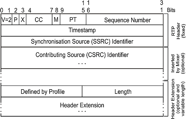
RTP header
Version (V): 2 bits. This field identifies the version of RTP. The current version is 2.
Padding (P): 1 bit. If the padding bit is set, the packet contains one or more additional padding bytes at the end which are not part of the payload. The last byte of the padding contains a count of how many padding bytes should be ignored. Padding may be needed by some encryption algorithms with fixed block sizes or for carrying several RTP packets in a lower-layer protocol data unit.
Extension (X): 1 bit. If the extension bit is set, the fixed header is followed by exactly one header extension, with a format defined in RFC 1889 Section 5.3.1.
CSRC count (CC): 4 bits. The CSRC count contains the number of CSRC identifiers that follow the fixed header.
Marker (M): 1 bit. The interpretation of the marker is defined by a profile. It is intended to allow significant events such as frame boundaries to be marked in the packet stream.
Payload type (PT): 7 bits. This field identifies the format of the RTP payload and determines its interpretation by the application. A profile specifies a default static mapping of payload type codes to payload formats.
Sequence number: 16 bits. The sequence number increments by one for each RTP data packet sent, and may be used by the receiver to detect packet loss and to restore packet sequence. The initial value of the sequence number is random (unpredictable) to make known plaintext attacks on encryption more difficult, even if the source itself does not encrypt, because the packets may flow through a translator that does.
Timestamp: 32 bits. The timestamp reflects the sampling instant of the first byte in the RTP data packet. The sampling instant must be derived from a clock that increments monotonically and linearly in time to allow synchronization and jitter calculations. The resolution of the clock must be sufficient for the desired synchronization accuracy and for measuring packet arrival jitter (one tick per video frame is typically not sufficient). The clock frequency is dependent on the format of data carried as payload and is specified statically in the profile or payload format specification that defines the format, or may be specified dynamically for payload formats defined through non-RTP means. The initial value of the timestamp is random, as for the sequence number. Several consecutive RTP packets may have equal timestamps if they are (logically) generated at once, e.g., belong to the same video frame. Consecutive RTP packets may contain timestamps that are not monotonic if the data is not transmitted in the order it was sampled, as in the case of MPEG interpolated video frames.
SSRC: 32 bits. The SSRC field identifies the synchronization source. This identifier is chosen randomly, with the intent that no two synchronization sources within the same RTP session will have the same SSRC identifier.
CSRC list: 0 to 15 items, 32 bits each. The CSRC list identifies the contributing sources for the payload contained in this packet. The number of identifiers is given by the CC field. If there are more than 15 contributing sources, only 15 may be identified. CSRC identifiers are the SSRC identifiers of contributing sources. For example, for audio packets the SSRC identifiers of all sources that were mixed together to create a packet are listed, allowing correct talker indication at the receiver.
RTP header extension. An extension mechanism is provided to allow individual implementations to experiment with new payload-format-independent functions that require additional information to be carried in the RTP data packet header.
13.2.3 RTCP
The Real-Time Control Protocol (RTCP) is based on the periodic transmission of control packets to all participants in the session, using the same distribution mechanism as the data packets. The underlying protocol must provide multiplexing of the data and control packets, for example using separate port numbers with UDP. RTCP performs the following functions.
The primary function is to provide feedback on the quality of the data distribution. This is an integral part of RTP’s role and is related to the flow and congestion control functions of other transport protocols. The feedback may be directly useful for control of adaptive encoding, but experiments with IP multicasting have shown that it is also critical to get feedback from the receivers to diagnose faults in the distribution. Sending reception feedback reports to all participants allows a person who is observing problems to evaluate whether those problems are local or global. With a distribution mechanism like IP multicast, it is also possible for an entity such as an ISP who is not otherwise involved in the session to receive the feedback information and act as a third-party monitor to diagnose network problems. This feedback function is performed by the RTCP sender and receiver reports and is described in RFC 1889 Section 6.3.
RTCP carries a persistent transport-level identifier for an RTP source called the ‘canonical name’ or CNAME. Since the SSRC identifier may change if a conflict is discovered or a program is restarted, receivers require the CNAME to keep track of each participant. Receivers also require the CNAME to associate multiple data streams from a given participant in a set of related RTP sessions, for example to synchronies audio and video.
The first two functions require that all participants send RTCP packets, therefore the rate must be controlled in order for RTP to scale up to a large number of participants. By having each participant send its control packets to all the others, each can independently observe the number of participants. This number is used to calculate the rate at which the packets are sent.
A fourth, optional function is to convey minimal session control information, for example participant identification to be displayed in the user interface. This is most likely to be useful in ‘loosely controlled’ sessions where participants enter and leave without membership control or parameter negotiation. RTCP serves as a convenient channel to reach all the participants, but it is not necessarily expected to support all the control communication requirements of an application.
RTCP packet format
This specification defines several RTCP packet types to carry a variety of control information, namely:
- SR: A Sender Report, for transmission and reception statistics from participants that are active senders
- RR: a Receiver Report, for reception statistics from participants that are not active senders
- SDES: Source description items, including CNAME
- BYE: Indicates end of participation
- APP: Application specific functions
Each RTCP packet begins with a fixed part, similar to that of RTP data packets, followed by structured elements that may be of variable length according to the packet type but always end on a 32-bit boundary. The alignment requirement and a length field in the fixed part are included to make RTCP packets ‘stackable’. Multiple RTCP packets may be concatenated without any intervening separators to form a compound RTCP packet that is sent in a single packet of the lower layer protocol, for example UDP. There is no explicit count of individual RTCP packets in the compound packet since the lower layer protocols are expected to provide an overall length to determine the end of the compound packet.
For further details on RTCP refer to RFC 1889 and RFC 1890.
13.2.4 SDP
The Session Description Protocol, SDP (RFC 2327), is a session description protocol for multimedia sessions. A multimedia session, for these purposes, is defined as a set of media streams that exist for some duration of time. Media streams can be many-to-many and the times during which the session is active need not be continuous.
SDP is used for purposes such as session announcement or session invitation. On the Internet Multicast Backbone (MBone), SDP is used to advertise multimedia conferences and communicate the conference addresses and conference tool-specific information necessary for participation. The MBone is the part of the Internet that supports IP multicast, and thus permits efficient many-to-many communication. It is used extensively for multimedia conferencing.
SDP is purely a format for session description. It does not incorporate a transport protocol and has to use different transport protocols as appropriate, including the Session Announcement Protocol (SAP), Session Initiation Protocol (SIP), Real-Time Streaming Protocol (RTSP), email using the MIME extensions, and the Hypertext Transport Protocol (HTTP).
A common approach is for a client to announce a conference session by periodically multicasting an announcement packet to a well-known multicast address and port using the Session Announcement Protocol (SAP). An SAP packet consists of an SAP header with a text payload, which is an SDP session description no greater than 1 Kbytes in length. If announced by SAP, only one session announcement is permitted in a single packet.
Alternative means of conveying session descriptions include email and the World Wide Web. For both email and WWW distribution, the use of the MIME content type ‘application/sd’ is used. This enables the automatic launching of applications for participation in the session from the browser or mail reader.
SDP serves two primary purposes. It is a means to communicate the existence of a session, as well as a means to convey sufficient information to enable joining and participating in the session. In this regard SDP includes information such as the session name and purpose, the time(s) the session is active, the media comprising the session, information to receive those media (addresses, ports, formats etc.), information about the bandwidth to be used by the conference, and contact information for the person responsible for the session.
Detailed information regarding the media include the type of media (video, audio, etc), the transport protocol (RTP, UDP, IP, H.320, etc), as well as the format of the media (H.261 video, MPEG video, etc).
For an IP multicast session, the multicast address as well as the port number for media are supplied. This IP address and port number are the destination address and destination port of the multicast stream, whether being sent, received, or both. For an IP unicast session, the remote IP address for media as well as the port number for the contact address is supplied.
Sessions may either be bounded or unbounded in time. Whether or not they are bounded, they may be only active at specific times. With regard to timing information, SDP can convey an arbitrary list of start and stop times bounding the session. It can also include repeat times for each bound, such as ‘every Monday at 10am for one hour’. This timing information is globally consistent, irrespective of local time zone or daylight saving time.
13.2.5 RTSP
The Real-Time Streaming Protocol (RTSP) is an Application layer protocol that establishes and controls either a single or several time-synchronized streams of continuous media such as audio and video. It normally does not deliver the continuous streams itself, although interleaving of the continuous media stream with the control stream is possible. In other words, RTSP acts as a ‘network remote control’ for multimedia servers.
There is no notion of an RTSP connection. Instead, a server maintains a session labeled by an identifier. An RTSP session is not tied to a transport-level connection such as a TCP connection. During an RTSP session, an RTSP client may open and close many reliable transport connections to the server to issue RTSP requests. Alternatively, it may use a connectionless transport protocol such as UDP.
The streams controlled by RTSP may use RTP, but the operation of RTSP does not depend on the transport mechanism used to carry continuous media. The protocol is intentionally similar in syntax and operation to HTTP version 1.1 so that extension mechanisms to HTTP can, in most cases, also be added to RTSP. However, RTSP differs fundamentally from HTTP/1.1in that data delivery takes place ‘out-of-band’ in a different protocol. HTTP is an asymmetric protocol where the client issues requests and the server responds. In RTSP, both the media client and media server can issue requests. RTSP requests are also not stateless; they may set parameters and continue to control a media stream long after the request has been acknowledged.
- The protocol supports the following operations:
Retrieval of media from a media server. The client can request a presentation description via HTTP or some other method. If the presentation is being multicast, the presentation description contains the multicast addresses and ports to be used for the continuous media. If the presentation is to be sent only to the client via unicast, the client provides the destination for security reasons. - Invitation of a media server to a conference. A media server can be ‘invited’ to join an existing conference, either to play back media into the presentation or to record all or a subset of the media in a presentation. This mode is useful for distributed teaching applications. Several parties in the conference may take turns ‘pushing the remote control buttons.’
- Addition of media to an existing presentation. Particularly for live presentations, it is useful if the server can tell the client about additional media becoming available.
13.2.6 RSVP
The need for a Quality of Service (QoS) on the Internet arose because of the increasing number of time-sensitive applications involving voice and video. RSVP (RFC 2205) is a resource reservation set-up protocol designed for that purpose. It is used by a host to request specific qualities of service from the network for particular application data streams or flows. It is also used by routers to deliver QoS requests to all nodes along the path(s) of the flows and to establish and maintain the requested service. RSVP requests will generally result in resources being reserved in each node along the data path.
RSVP requests resources for ‘simplex’ flows, i.e. it requests resources in only one direction. Therefore, RSVP treats a sender as logically distinct from a receiver, although the same application process may act as both a sender and a receiver at the same time. RSVP operates on top of IPv4 or IPv6, occupying the place of a transport protocol in the protocol stack. However, RSVP does not transport application data, but rather an Internet control protocol such as ICMP, IGMP, or routing protocols. Like the implementations of routing and management protocols, an implementation of RSVP will typically execute in the background and not in the data path.
RSVP is not itself a routing protocol. Instead, it is designed to operate with current and future unicast and multicast routing protocols. An RSVP process consults the local routing database(s) to obtain routes. In the multicast case, for example, a host sends IGMP messages to join a multicast group and then sends RSVP messages to reserve resources along the delivery path(s) of that group whereas routing protocols determine where packets get forwarded. RSVP, however, is only concerned with the QoS of those packets that are forwarded in accordance with routing decisions.
QoS is implemented for a particular data flow by mechanisms collectively called ‘traffic control’. These mechanisms include a packet classifier, admission control, and a packet scheduler or some other Data Link layer-dependent mechanism to determine when particular packets are forwarded. The packet classifier determines the QoS class (and perhaps the route) for each packet. For each outgoing interface, the packet scheduler or other Data Link layer-dependent mechanism achieves the promised QoS. Traffic control implements QoS service models defined by the Integrated Services Working Group.
RSVP does the following:
- It makes resource reservations for both unicast and many-to-many multicast applications, adapting dynamically to changing group membership as well as to changing routes.
- It operates in simplex mode, i.e., it makes reservations for unidirectional data flows.
- It is receiver-oriented, i.e., the receiver of a data flow initiates and maintains the resource reservation used for that flow.
- It maintains ‘soft’ state in routers and hosts, providing support for dynamic membership changes and automatic adaptation to routing changes.
- It is not a routing protocol, but depends on present and future routing protocols.
- It transports and maintains traffic control and policy control parameters that are opaque to RSVP.
- It provides several reservation models or ‘styles’ to fit a variety of applications.
- It provides transparent operation through routers that do not support it.
- It supports both IPv4 and IPv6.
The RSVP message consists of 3 sections namely a Common Header (8 bytes), an Object Header (4 bits) and Object Contents (variable length).
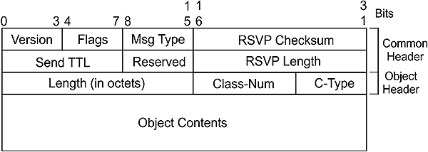
RSVP header
The Version field (4 bits) contains the current version, which is 2.
The Flags field (4 bits) is reserved for future use.
The Message Type (1 byte) indicates 1 of 7 currently defined messages. They are:
- Type 1: Path Messages. Each sender host periodically sends a Path message for each data flow it originates. A Path message travels from a sender to receiver(s) along the same path(s) used by the data packets.
- Type 2: Resv Messages. Resv (reservation) messages carry reservation requests hop-by-hop from receivers to senders, along the reverse paths of data flows for the session.
- Type 3: PathErr Messages. PathErr (path error) messages report errors in processing Path messages. They travel upstream towards senders and are routed hop-by-hop using the path state. PathErr messages do not modify the state of any node through which they pass; they are only reported to the sender application.
- Type 3: ResvErr Messages. ResvErr (reservation error) messages report errors in processing Resv messages, or they may report the spontaneous disruption of a reservation, e.g., by administrative pre-emption. ResvErr messages travel downstream towards the appropriate receivers, routed hop-by-hop using the reservation state.
- Type 5/6: Teardown Messages. RSVP ‘teardown’ messages remove path or reservation states immediately. Although it is not necessary to explicitly tear down an old reservation, it is recommended that all end hosts send a teardown request as soon as an application finishes. There are two types of RSVP teardown message, namely PathTear (5) and ResvTear (6). A PathTear message travels towards all receivers downstream from its point of initiation and deletes path states, as well as all dependent reservation states, along the way. A ResvTear message deletes reservation states and travels towards all senders upstream from its point of initiation.
- Type 7: ResvConf Messages. ResvConf (reservation conformation) messages are sent to acknowledge reservation requests and are forwarded to the receiver hop- by-hop, to accommodate the hop-by-hop integrity check mechanism.
The RSVP Checksum field (2 bytes) provides error control.
The Send_TTL field (1byte) is the IP Time-to-Live value with which the message was sent.
The RSVP length field (2 bytes) is the total length of the RSVP message in bytes.
Each Object consists of one or more 32 bit long words with a 1 byte Object Header. The Object contents are fairly complex and beyond the scope of this document and readers are referred to RFC 2205 for details.
13.2.7 Summary
The following sketch summarizes the protocol stack implementation. It shows a 20mS voice sample from a codec, preceded by an RTP, UDP, IP and Ethernet Header. Note that the drawing is not upside-down, but has been drawn according to the actual sequence in which the bytes are transmitted. The operation of the coders and decoders (codecs) are discussed in the following paragraphs.

VoIP summary
13.3 Hardware
13.3.1 Introduction
The Voice over IP Forum (part of the International Multimedia Teleconferencing Consortium) has developed an Implementation Agreement that describes several connectivity configurations for converged networks. These configurations are summarized in Fig 9.1. It allows for:
- PC to PC connection
- Phone to phone connection over IP, and
- PC to phone connection.
All components shown, with the exception of the DNS server, adhere to the H.323 standard.

Elements used for PC/telephone interconnection.
13.3.2 H.323 overview
The ITU-T H.323 (Packet Based Multimedia Communication Systems) standard deals with the components, protocols, and procedures required for the transmission of real-time audio, video, and data communications over packet-based networks including IP or IPX- based LANs, MANs, WANs and VPNs. H.323 can be used for audio only (IP telephony), audio/video (video telephony), audio/data, and audio/video/data. H.323 can also be applied to multipoint-multimedia communications.
The H.323 standard deals with visual telephone systems and equipment for LANs that provide a non-guaranteed QoS and it is part of the H.32x family of ITU–T standards. Other standards in the family include:
- H.320 Narrowband visual telephone systems and Terminal equipment (used with ISDN)
- H.321 Adaptation of H.320 Terminals to Broadband ISDN (B-ISDN)
- H.322 Visual telephone systems and equipment for local area networks that provide a guaranteed QoS
- H.324 Terminal for low bit rate multimedia communications (used with PSTN and wireless applications).
In addition to the network implementation standards mentioned above, there are other standards that fall under the umbrella of the H.323 recommendation. These include:
- H.225.0 Terminal to Gatekeeper functions
- H.245 Terminal control functions used to negotiate channel capabilities and usage
- Q.931 Call signaling functions to establish and terminate a call
- T.120 Data conferencing, including whiteboarding and still image functions
13.3.3 H.323 building blocks
The H.323 standard specifies four kinds of components that, when networked together, provide the point-to-point and point-to-multipoint multimedia-communication services. They are:
- Terminals,
- Gateways,
- Gatekeepers and
- Multipoint Control Units (MCUs)
Terminals
Terminals are used for real-time bi-directional multimedia communications. An H.323 Terminal can either be a PC or a stand-alone device, running an H.323 stack and multimedia applications. By default a Terminal supports audio communications and it can optionally support video or data communications. H.323 Terminals may be used in multi-point conferences.
The primary goal of H.323 is to inter-network multimedia Terminals and for this reason H.323 Terminals are compatible with H.324 Terminals on switched-circuit networks (PSTN) and wireless networks, H.310 Terminals on B–ISDN, H.320 Terminals on ISDN, H.321 Terminals on B–ISDN, and H.322 Terminals on guaranteed QoS LANs
Gateways
One of the primary goals in the development of the H.323 standard was interoperability between an H.323 network and any other non-H.323 multimedia-services network such as a PSTN network. This is achieved through the use of a Gateway, which performs any network or signaling translation required between the two networks. This connectivity of dissimilar networks is achieved by translating protocols for call set-up and release, converting media formats between different networks, and transferring information between the networks connected by the gateway.
Gatekeepers
A Gatekeeper can be considered the ‘brain’ of the H.323 network and is the focal point for all calls within the H.323 network. Although not mandatory, Gatekeepers provide important services such as addressing, authorization and authentication of Terminals and gateways, bandwidth management, accounting, billing, charging and call-routing services.
Multipoint Control Units
MCUs provide support for conferences of three or more H.323 Terminals. All Terminals participating in the conference establish a connection with the MCU. The MCU manages conference resources, negotiates between Terminals for the purpose of determining the audio or video CODEC to use, and may handle the media stream. The Gatekeepers, Gateways, and MCUs are logically separate components of the H.323 standard but can be implemented as a single physical device.
Zones
An H.323 Zone is not a building block, bur rather a collection of all Terminals, Gateways, and MCUs managed by a single Gatekeeper. A zone includes at least one Terminal and may include Gateways or MCUs, but only one Gatekeeper. A zone is independent of network topology and may comprise multiple network segments that are connected using routers, switches or bridges.
H.323 Zone
13.3.4 H.323 protocols
The protocols specified by H.323 are listed below. H.323 is, however, independent of the Physical, data link, Network and Transport layer protocols over which it runs and does not specify them.
- Audio codecs
- Video codecs
- H.225 Registration, Admission and Status (RAS)
- H.225 call signaling
- H.245 control signaling
- Real-time Transfer Protocol (RTP)
- Real-time Control Protocol (RTCP)
Here follows brief descriptions of these protocols.
Audio (voice) codecs
In order to transport the analog voice signal, it has to be digitized. The traditional approach is to sample it at 8000 samples per second, and then to quantize each sample into an 8 bit digital value, with a resolution of 1/(28) = 1/256. Thus the basic bit rate becomes 8,000 samples/second x 8 bits/sample = 64,000 bits/second, known as the DS0 rate. Through an additional process, called encoding, the 64,000 bits/second bandwidth requirement can be reduced considerably, by employing techniques such as data compression, silence suppression and voice activity detection. On the receiving side the process has to be reversed.
An audio codec encodes the audio signal from the microphone for transmission on the transmitting H.323 Terminal and decodes the received audio code on the receiving H.323 Terminal. Because audio is the minimum service provided by the H.323 standard, all H.323 Terminals must have at least one audio codec support, as specified in the ITU–T G.711 (1972) recommendation. This algorithm operates at 64 Kbps, using PCM to produce a frame that contains 125 microseconds of speech. No compression is used.
Additional CODECS that may be supported include:
- G.722 (1988). Operates at 64, 56, or 48 Kbps and is known as the wideband coder.
- G.723.1 (1995). Operates at 5.3 and 6.3 Kbps. Algebraic Code Excited Linear Prediction (ACELP) is used for the lower rate and Multi-pulse Maximum Likelihood Quantization (MP-MLQ) is used for the higher rate.
- G.726 (1990). Operates at 16, 24, 32 and 40 Kbps, and uses Adaptive Differential Pulse Code Modulation (ADPCM).
- G.728 (1995). Operates at 16 Kbps and uses Conjugate Structure Algebraic Code Excited Linear Prediction (CS-ACELP).
- G.729 (1996) Operates at 8kbps and uses a less complex version of CS-ACELP.

Packet telephony
Video codecs
A video codec encodes video from a camera for transmission on the transmitting H.323 Terminal and decodes the received video code on the receiving H.323 Terminal. H.323 specifies support of video, and hence video codecs, as optional. However, H.323 Terminals providing video communications must support video encoding and decoding as specified in the ITU–T H.261 recommendation. H.261 operates at multiples of 64 x p Kbps, where p varies from 1 to 30, resulting in bit rates from 40 Kbps to 2 Mbps
An alternative is H.263, based on H.261, which introduces additional compression. It contains negotiable options and can operate on a number of different video formats.
H.225 Registration, Admission and Status
Registration, Admission and Status (RAS) is the protocol used between H.323 endpoints (Terminals/ Gateways) and Gatekeepers for Gatekeeper discovery, Endpoint registration, Endpoint location and Admission control.
A RAS signaling channel, opened between an endpoint and a Gatekeeper prior to the establishment of any other channels, is used to exchange RAS messages. This channel is unreliable; hence RAS message exchange may be associated with timeouts and retry counts.
The Gatekeeper discovery (GRQ) process is used by the H.323 endpoints to determine the Gatekeeper with which the endpoint must register and can be done statically or dynamically. In static discovery, the endpoint knows the transport address of its Gatekeeper in advance. In the dynamic method of Gatekeeper discovery, the endpoint multicasts a GRQ message on the Gatekeeper’s discovery multicast address: ’Who is my Gatekeeper?’ One or more Gatekeepers may respond with a GCF message: ‘I can be your Gatekeeper.’
Registration is a process used by the endpoints to join a zone and inform the Gatekeeper of the zone’s transport and alias addresses. All endpoints register with a Gatekeeper as part of their configuration.
Endpoint location is a process by which the transport address of an endpoint is determined and given its alias name or E.164 address.
The RAS channel is used for other kinds of control mechanisms, such as admission control, to restrict the entry of an endpoint into a zone, bandwidth control, and disengagement control, where an endpoint is disassociated from a Gatekeeper and its zone.
H.225 Call signaling
H.225 call signaling is used to establish a connection between two H.323 endpoints over which the real-time data can be transported. This is achieved by exchanging H.225 protocol messages on the call-signaling channel. The call-signaling channel is opened between two H.323 endpoints or between an endpoint and the Gatekeeper.
Call signaling involves the exchange of H.225 protocol messages over a reliable call-signaling channel; hence H.225 protocol messages are carried over TCP in an IP-based H.323 network. H.225 messages are exchanged between the endpoints if there is no Gatekeeper in the H.323 network. When a Gatekeeper exists in the network, the H.225 messages are exchanged either directly between the endpoints or between the endpoints after being routed through the Gatekeeper. The first case is called direct call signaling. The second case is called Gatekeeper-routed call signaling. The method chosen is decided by the Gatekeeper during RAS–admission message exchange.
In the case of Gatekeeper-routed call signaling the admission messages are exchanged between endpoints and the Gatekeeper on RAS channels. The Gatekeeper receives the call-signaling messages on the call-signaling channel from one endpoint and routes them to the other endpoint on the call-signaling channel of the other endpoint.
Direct call signaling is used if, during the admission confirmation, the Gatekeeper indicates that the endpoints can exchange call-signaling messages directly. The endpoints then exchange the call signaling on the call-signaling channel.
H.245 control signaling
H.245 control signaling is used to exchange end-to-end control messages governing the operation of the H.323 endpoints. These control messages carry information related to capabilities exchange, opening and closing of logical channels used to carry media streams, flow-control messages and general commands and indications.
The H.245 control messages are carried over H.245 control channels. The H.245 control channel is the logical channel 0 and is permanently open, unlike the media channels. The messages carried include messages to exchange capabilities of Terminals and to open and close logical channels.
Capabilities exchange is a process whereby the communicating Terminals exchange messages to provide their transmit and receive capabilities to the peer endpoints. Transmit capabilities describe a Terminal’s ability to transmit media streams, whereas Receive capabilities describe a Terminal’s ability to receive and process incoming media streams.
A logical channel carries information from one endpoint to another endpoint (in the case of a point-to-point conference) or multiple endpoints (in the case of a point-to-multipoint conference). H.245 provides messages to open or close a logical channel; a logical channel is unidirectional.
RTP
RTP provides end-to-end delivery services of real-time audio and video using UDP. It provides payload-type identification, sequence numbering, time stamping, delivery monitoring, multiplexing and checksum services. RTP is discussed in detail in the beginning of this chapter.
RTCP
RTCP is the counterpart of RTP that provides control services. The primary function of RTCP is to provide feedback on the quality of the data distribution. Other functions include carrying a transport-level identifier for an RTP source, called a canonical name, which is used by receivers to synchronies audio and video. RTCP is discussed in detail in the beginning of this chapter.
13.3.5 Terminal implementation
Terminals implement the following protocols:
- H.245 for exchanging Terminal capabilities and creation of media channels
- H.225 for call signaling and call set-up
- RAS for registration and other admission control with a Gatekeeper
- RTP/RTCP for sequencing audio and video packets
H.323 Terminals must also support the G.711 audio codec. Optional components in an H.323 Terminal are video codecs and T.120 data-conferencing protocols.

Terminal protocol stack
13.3.6 Gateway implementation
Gateways provide translation of protocols for call set-up and release, conversion of media formats between different networks, and the transfer of information between H.323 and non-H.323 networks. An application of the H.323 Gateways is in IP telephony, where the H.323 Gateways connect IP networks and Switched Circuit Networks (SCNs) e.g. PSTN and ISDN networks.
On the H.323 side, a Gateway runs H.245 control signaling for exchanging capabilities, H.225 call signaling for call set-up and release, and H.225 RAS for registration with the Gatekeeper. On the SCN side, a Gateway runs SCN-specific protocols e.g. ISDN and SS7. Terminals communicate with the Gateway using the H.245 control-signaling and H.225 call-signaling protocols. The Gateway translates these protocols in a transparent fashion to the respective counterparts on the non-H.323 network and vice versa. The Gateway also performs call set-up and clearing on both the H.323-network side and the non-H.323 network side. Translation between audio, video, and data formats may also be performed by the Gateway. Audio and video translation may not be required if both Terminal types find a common communications mode. For example, in the case of Gateways to H.320 Terminals on ISDN, both Terminal types require G.711 audio and H.261 video, so a common mode always exists. The Gateway has the characteristics of both an H.323 Terminal on the H.323 network and the other Terminal on the non-H.323 network it connects. Gatekeepers are aware of which endpoints are Gateways because this is indicated when the Terminals and Gateways register with the Gatekeeper. A Gateway may be able to support several simultaneous calls between the H.323 and non-H.323 networks. A Gateway is a logical component of H.323 and can be implemented as part of a Gatekeeper or an MCU.

Gateway protocol stack
13.3.7 Gatekeeper implementation
Gatekeepers provide call-control services for H.323 endpoints, such as address translation and bandwidth management as defined within RAS, and are optional. If they are present in a network, however, Terminals and Gateways must use their services. The H.323 standards define both mandatory services that the Gatekeeper must provide, as well as other optional functionality that it may provide. An optional feature of a Gatekeeper is call-signaling routing. Endpoints send call-signaling messages to the Gatekeeper, which the Gatekeeper routes to the destination endpoints. Alternately, endpoints can send call-signaling messages directly to the peer endpoints. This feature of the Gatekeeper is valuable, as monitoring of the calls by the Gatekeeper provides better control of the calls in the network. Routing calls through a Gatekeeper provides better performance in the network, as the Gatekeeper can make routing decisions based on a variety of factors, for example, load balancing among Gateways. The services offered by a Gatekeeper are defined by RAS and include address translation, admissions control, bandwidth control, and zone management. H.323 networks that do not have Gatekeepers may not have these capabilities, but H.323 networks that contain IP-telephony Gateways should contain a Gatekeeper to translate incoming E.164 telephone addresses into transport addresses. A Gatekeeper is a logical component of H.323 but can be implemented as part of a Gateway or MCU.

Gatekeeper protocol stack
Mandatory Gatekeeper functions
These are mandatory functions.
- Address translation
- Calls originating within an H.323 network may use an alias to address the destination Terminal. Calls originating outside the H.323 network and received by a Gateway may use an E.164 telephone number (e.g. 310-442-9222) to address the destination Terminal. The Gatekeeper translates this number or the alias into the network address (e.g. 204.252.32.116 for an IP-based network) for the destination Terminal. The destination endpoint can be reached using the network address on the H.323 network.
- Admissions control
- The Gatekeeper can control the admission of the endpoints into the H.323 network. It uses RAS messages as specified in H.225.0 such as Admission ReQuest (ARQ), Admission ConFirm (ACF), and Admission ReJect (ARJ) to achieve this. Admissions control may be a null function that admits all endpoints to the H.323 network.
- Bandwidth control
- The Gatekeeper provides support for bandwidth control by using the RAS (H.225.0) messages Bandwidth ReQuest (BRQ), Bandwidth ConFirm (BCF), and Bandwidth ReJect (BRJ). For instance, if a network manager has specified a threshold for the number of simultaneous connections on the H.323 network, the Gatekeeper can refuse to make any more connections once the threshold is reached. The result is to limit the total allocated bandwidth to some fraction of the total available, leaving the remaining bandwidth for data applications. Bandwidth control may also be a null function that accepts all requests for bandwidth changes.
- Zone management
- The Gatekeeper provides the above functions viz. address translation, admissions control and bandwidth control for Terminals, Gateways, and MCUs located within its zone of control.
Optional Gatekeeper functions
- Call-control signaling
- The Gatekeeper can route call-signaling messages between H.323 endpoints. In a point-to-point conference, the Gatekeeper may process H.225 call-signaling messages. Alternatively, the Gatekeeper may allow the endpoints to send H.225 call-signaling messages directly to each other.
- Call authorization
- When an endpoint sends call-signaling messages to the Gatekeeper, the Gatekeeper may accept or reject the call, according to the H.225 specification. The reasons for rejection may include access-based or time-based restrictions, to and from particular Terminals or Gateways.
- Call management
- The Gatekeeper may maintain information about all active H.323 calls so that it can control its zone by providing the maintained information to the bandwidth-management function or by re-routing the calls to different endpoints to achieve load balancing.
13.4 Implementation considerations: QoS
QoS is defined in ITU-T E.800 as ‘The collective effect of service performance, which determines the degree of satisfaction of a user of the service.’ Unfortunately this is a very subjective evaluation, but there are several techniques for evaluating QoS such as the Conversation Opinion test outlined in ITU-T P.800. This test uses volunteers to rate the quality of a telephone connection from 1 to 5 where 1 is bad, 2 is poor, 3 is fair, 4 is good and 5 is excellent.
13.4.1 Factors influencing QoS.
In a VoIP conversation between a telephone and a PC situated at home, the voice signal has to pass through six distinct subsystems namely the telephone client, PSTN, Gateways, IP network, dial-up link and PC client.
Each leg of the journey adds some delay, which is noticeable on VoIP connections. In addition, the IP network could add some packet loss, and also some packet jitter due to packets traveling on different routes and therefore not spending the same amount of time within the network.

Factors introducing delays
13.4.2 Integrated services
Integrated Services (‘int-serv’) as described in RFC 1633 is a model developed by the IETF. An end station that supports RSVP can request that bandwidth be reserved along a specific path, prior to the transmission of the data. RSVP has been designed to work in conjunction with routing protocols such as OSPF and BGP-4, and rely on these to decide where the reservation requests should be sent. There are four components in the Integrated Services model, namely RSVP, an Admission Control Routine that determines if network resources are available, a Classifier that puts packets in specific queues, and a Packet Scheduler that schedules packets to meet QoS requirements.
13.4.3 Differentiated Services
Differentiated Services (‘diff-serv’) as described in RFC 2474 was also developed by the IETF. It distinguishes packets that require different network services into different classes, identified by an 8-bit Differentiated Services (DS) field. This field then replaces the Type of Service field in the IPv4 header, or the Traffic Class field in the IPv6 header. It is assumed that ISPs will be able to offer different types of service, at different costs, based on the DS field.
13.4.4 Multiprotocol Label Switching
Multiprotocol Label Switching (MPLS) is described in RFC 2702. In a so-called MPLS domain, in which all routers are Label Switching Routers or LSRs (i.e. MPLS capable), all packets entering the domain are modified by inserting a 32 bit header (‘tag’) between the local network (e.g. Ethernet) header and the IP header. Packets are classified at the ingress LSR, and subsequently handled on the information contained in the tag and not the IP header. This means that this mechanism is independent of the Network layer protocol being used.
13.4.5 Queuing and congestion avoidance mechanisms
Queuing mechanisms employed on routers classify incoming data flows according to attributes such as source and destination IP addresses, protocol used, or port number. It then lines them up in multiple parallel queues according to their classification. It then grants each of these individual flows a percentage of the available bandwidth.
Congestion mechanisms try to prevent data from being sent to already congested routes. This is done by using mechanisms such as Random Early Detection (RED) to predict when congestion will occur, rather than leaving it up to TCP’s built-in mechanism which causes packets to be dropped when congestion eventually does occur.
Objectives
When you have completed study of this chapter you should be able to:
- Explain the security problem
- Define the ways of controlling access to a network
14.1 The security problem
Although people tend to refer to the ‘Internet’ as one global entity, there are in fact three clearly defined subsets of this global network. Four, in fact, if one wishes to include the so-called ‘community network’. It just depends on where the conceptual boundaries are drawn.
- In the center is the in-house corporate ‘intranet’, primarily for the benefit of the people within the organization
- The intranet is surrounded by the ‘extranet’, exterior to the organization yet restricted to access by business partners, customers and preferred suppliers
- Third (optionally), there can be a ‘community’ layer around the extranet. This space is shared with a particular community of interest, e.g. industry associations
- Finally, these three layers are surrounded by the global Internet as we know it, which is shared by prospective clients/customers and the rest of the world
This expansion of the Internet into organizations, in fact right down to the factory floor, has opened the door to incredible opportunities. Unfortunately it has also opened the door to pirates and hackers. Therefore, as the use of the Internet has grown, so has the need for security. The TCP/IP protocols and network technologies are inherently designed to be open in order to allow interoperability. Therefore, unless proper precautions are taken, data can readily be intercepted and altered – often without the sending or the receiving party being aware of the security breach. Because dedicated links between the parties in a communication are often not established in advance, it is easy for hackers to impersonate one of the parties involved.
There is a misconception that attacks on a network will always take place from the outside. This is as true of networks as it is true of governments. The growth in network size and complexity has increased the potential points of attack both from outside and from within.
Without going into too much detail, the following list attempts to give an idea of the magnitude of the threat experienced by intranets and extranets:
- Unauthorized access by contractors or visitors to a company’s computer system
- Access by authorized users (employees or suppliers) to unauthorized databases. For example, an engineer might break into the Human Resources database to obtain confidential salary information
- Confidential information might be intercepted as it is being sent to an authorized user. A hacker might attach a network-sniffing device (probe) to the network, or use sniffing software on his computer. While sniffers are normally used for network diagnostics, they can also be used to intercept data traveling over the network medium
- Users may share documents between geographically separated offices over the Internet or extranet, or ‘telecommuters’ users accessing the corporate intranet from their home computer via a dial-up connection can expose sensitive data as it is sent over the medium
- E-mail can be intercepted in transit, or hackers can break into the mail server
Here follows a list of some additional threats:
- SYN flood attacks
- Fat ping attacks (ping of death)
- IP spoofing
- Malformed packet attacks (TCP and UDP)
- ACK storms
- Forged source address packets
- Packet fragmentation attacks
- Session hijacking
- Log overflow attacks
- SNMP attacks
- Log manipulation
- ICMP broadcast flooding
- Source routed packets
- ARP attacks
- Ghost routing attacks
- Sequence number prediction
- FTP bounce or port call attack
- Buffer overflows
- ICMP protocol tunneling
- VPN key generation attacks
These are not merely theoretical concerns. While computer hackers breaking into corporate computer systems over the Internet have received a great deal of press in recent years, in reality insiders such as employees, former employees, contractors working on- site and other suppliers are far more likely to attack their own company’s computer systems via an intranet. In a 1998 survey of 520 security practitioners in US corporations and other institutions conducted by the Computer Security Institute (CSI) with the participation of the FBI, 44 per cent reported unauthorized access by employees compared with 24 per cent reporting system penetration from the outside!
Such insider security breaches are likely to result in greater losses than attacks from the outside. Of the organizations that were able to quantify their losses, the CSI survey found that the most serious financial losses occurred through unauthorized access by insiders, with 18 companies reporting total losses of $51 million as compared with $86 million for the remaining 223 companies. The following list gives the average losses from various types of attacks as per the CSI/FBI Survey:
Table 14.1Financial losses due to cyber attacks
Fortunately technology has kept up with the problem, and the rest of this chapter will deal with possible solutions to the threat. Keep in mind that securing a network is a continuous process, not a one-time prescription drug that can be bought over the counter.
Also, remember that the most sensible approach is a defense-in-depth (‘belt-and-braces’) approach as used by the nuclear industry. In other words, one should not rely on a single approach, but rather a combination of measures with varying levels of complexity and cost.
14.2 Authentication
An organization whose LAN (or intranet) is not routed to the Internet mainly faces internal threats to its network. In order to allow access only to authorized personnel, authentication is often performed by means of passwords. A password, however, is mainly used to ‘keep the good guys out’ since it is usually very easy to figure out someone’s password, or to capture un-encrypted passwords with a protocol analyzer as they travel across the network.
To provide proper authentication, two or three items from the following list are required.
- Something the user knows. These can be a password or a PIN number, and by itself it is not very secure.
- Something the user has. This can be a SecurID tag, or similar. The SecurID system has a server on the network, generating a 6-bit pseudo-random code every 60 seconds. The user has a credit-card size card or a key fob with a 6-digit LCD display. After initialization at the server, the code on the user’s card follows the code on the server. After entering a PIN number, the prospective user enters the 6-digit code. Even if someone manages to obtain the code, it will be useless in less than a minute.
- Something the user is. This can be done with an iris or fingerprint scan. The hardware for this purpose is readily available.
There are several password authentication protocols in use, such as the Password Authentication Protocol (PAP) and the Challenge Handshake Authentication protocol (CHAP). However, the most secure method of authentication at this point in time is IEEE 802.1X port-based access control in conjunction with a RADIUS server. This is the case for wireless as well as wired access.
14.3 Routers
A router can be used as a simple firewall that connects the intranet to the ‘outside world’. Despite the fact that its primary purpose is to route packets, it can also assist in protecting the intranet.
In comparison to firewalls, routers are extremely simple devices and are clearly not as effective in properly securing a network perimeter access point. However, despite their lack of sophistication, there is much that can be done with routers to improve security on a network. In many cases these changes involve little administrative overhead.
There are two broad objectives in securing a router, namely:
- Protecting the router itself
- Using the router to protect the rest of the network
Protecting the router
The following approaches can be taken:
- Keep the router software current. This could be a formidable task, especially for managers maintaining a large routed network faced with the prospect of updating code on hundreds of devices. It is, however, essential since operating routers on current code is a substantial step toward protecting them from attack and properly maintaining security on a network. In addition, new updated software revisions often provide improved performance, offering more leeway to address security concerns without bringing network traffic to a halt
- It is imperative for network managers to keep current on release notes and vendor bulletins. Release notes are a good source of information and enable network managers to determine whether or not a fix is applicable to their network. In the case of a detected vulnerability in the software for a particular router, Computer Emergency Response Team (CERT) advisories and vendor bulletins often provide workarounds to minimize risk until a solution to the problem has been found
- Verify that the network manager’s password is strong and ensure that the password is changed periodically and distributed as safely and minimally as possible. More important, verify that all non-supervisory level accounts are password protected, to prevent unauthorized users from reading the router’s configuration information
- Allow TELNET access to the router only from specific IP addresses
- Authenticate any routing protocol possible
- From a security perspective, SNMP v1 and v2 lack authentication and privacy. This has been fixed with SNMP v3. However, defining a limited set of authorized SNMP management stations is always prudent
Protecting the network
- Logging
Logging the actions of the router can assist in completing the overall picture of the condition of the network. The ideal solution is to keep one copy of the log on the router, as well as one on a remote logging facility, such as Syslog, since an attacker could potentially fill the router’s limited internal log storage to erase details of the attack. With only remote storage, though, the attacker need only disrupt the logging service to prevent events from being recorded - Access Control Lists (ACLs)
ACLs allow the router to reject or pass packets based on TCP port number, IP source address or IP destination address. Traffic control can be accomplished on the basis of (a) implicit permission, which means only traffic not specifically prohibited will be passed through, or (b) implicit denial which means that all traffic not specifically allowed will be denied
14.4 Firewalls
Routers can be used to block unwanted traffic and therefore act as a first line of defense against unwanted network traffic, thereby performing basic firewall functions. It must, however, be kept in mind that they were developed for a different purpose, namely routing, and that their ability to assist in protecting the network is just an additional advantage. Routers, however sophisticated, generally do not make particularly intricate decisions about the content or source of a data packet. For this reason network managers have to revert to dedicated firewalls.
Firewalls can be one of the following types:
- Packet Filter
- Stateful Inspection
- Application Proxy gateway
- Dedicated Proxy server
- Hybrid type
We will review each of these types in detail.
14.4.1 Packet Filter firewalls
Packet Filter firewalls are essentially routing devices that include access control functionality for system addresses and communication sessions. The access control functionality of a Packet Filter firewall is governed by a set of directives collectively referred to as a rule-set. A typical rule-set is shown in table 6.1 below.
| S.No | Source address | Source port | Destination address | Destination port | Action | Description |
|---|---|---|---|---|---|---|
| 1 | Any | Any | 192.168.1.0 | >1023 | Allow | Rule to allow returning TCP connections to internal subnet |
| 2 | 192.168.1.1 | Any | Any | Any | Deny | Prevent Firewall system itself from directly connecting to anything |
| 3 | Any | Any | 192.168.1.1 | Any | Deny | Prevent external users from directly accessing the Firewall system. |
| 4 | 192.168.1.0 | Any | Any | Any | Allow | Internal users can access external servers |
| 5 | Any | Any | 192.168.1.2 | SMTP | Allow | Allow external users to send email in |
| 6 | Any | Any | 192.168.1.3 | HTTP | Allow | Allow external Users to access Internet |
| 7 | Any | Any | Any | Any | Deny | “Catch-all” rule – everything not previously allowed is explicitly denied |
Table 14.2
Typical rule-set of a Packet Filter firewallIn their most basic form, packet firewalls provide network access control based upon several pieces of information contained in a network packet:
- The source address of the packet, i.e. the layer 3 address of the computer system or device the network packet originated from (an IP address such as 192.168.1.1)
- The destination address of the packet, i.e. the layer 3 address of the computer system or device the network packet is trying to reach (e.g., 192.168.1.2)
- The type of traffic, that is, the specific network protocol being used to communicate between the source and destination systems or devices (often Ethernet at layer 2 and IP at layer 3)
- Possibly some characteristics of the layer 4 communications sessions, such as the source and destination ports of the sessions (e.g. TCP: 80 for the destination port belonging to a web server, TCP: 1320 for the source port belonging to a PC accessing the server)
- Sometimes, information pertaining to which interface of the router the packet came from and which interface of the router the packet is destined for. This is useful for routers with three or more network interfaces
Packet Filter firewalls are generally deployed within TCP/IP network infrastructures. In the context of modern network infrastructures, a firewall at layer 2 is used in load balancing and/or high-availability applications in which two or more firewalls are employed to increase throughput or for fail-safe operations. Packet Filtering firewalls and routers can also filter network traffic based upon certain characteristics of that traffic, such as whether the packet’s layer 3 protocol is ICMP. Attackers have used this protocol to flood networks with traffic, thereby creating Denial-Of-Service (DOS) attacks. Packet Filter firewalls also have the capability to block other attacks that take advantage of weaknesses in the TCP/IP suite.
Packet Filter firewalls have two main strengths: speed and flexibility. Since Packet Filters do not usually examine data above layer 3 of the OSI model, they can operate very fast. Likewise, since most modern network protocols can be accommodated using layer 3 and below, Packet Filter firewalls can be used to secure nearly any type of network communication or protocol. This simplicity allows Packet Filter firewalls to be deployed into nearly any enterprise network infrastructure. Their speed and flexibility, as well as their capability to block denial-of-service and related attacks, makes them ideal for placement at the outermost boundary of the trusted network. From that position it can block certain attacks, possibly filter unwanted protocols, perform simple access control, and then pass the traffic on to other firewalls that examine higher layers of the OSI stack.
Packet Filter firewalls also have a few shortcomings:
- Because Packet Filter firewalls do not examine upper-layer data, they cannot prevent attacks that employ application-specific vulnerabilities or functions. For example, a Packet Filter firewall cannot block specific application commands if a Packet Filter firewall allows a given application; all functions available within that application will be permitted
- Because of the limited information available to the firewall, the logging functionality present in Packet Filter firewalls is limited. Packet Filter logs normally contain the same information used to make access control decisions
- Most Packet Filter firewalls do not support advanced user authentication schemes. This limitation is mostly due to the lack of upper-layer functionality in the firewall
- They are generally vulnerable to attacks and exploits that take advantage of problems within the TCP/IP specification and protocol stack, such as network layer address spoofing. Many Packet Filter firewalls cannot detect a network packet in which the layer 3 addressing information has been altered. Spoofing attacks are generally employed by intruders to bypass the security controls implemented in a firewall platform
- Due to the small number of variables used in access control decisions, Packet Filter firewalls are susceptible to security breaches caused by improper or incorrect configurations
Packet Filter type firewalls are therefore limited to applications where logging and user authentication are not important issues, but where high speed is essential.
14.4.2 Stateful Inspection firewalls
Stateful Inspection firewalls are packet filters that incorporate added awareness of layer 4 (OSI model) protocols. Stateful Inspection evolved from the need to accommodate certain features of the TCP/IP protocol suite that make firewall deployment difficult. When a TCP (connection-oriented) application creates a session with a remote host system, a port is also created on the source system for the purpose of receiving network traffic from the destination system. According to the TCP specifications, this client source port will be some number greater than 1023 and less than 49151. According to convention, the destination port on the remote host will likely be a low-numbered port, less than 1024. This will be 25 for SMTP, for example. Packet Filter firewalls must permit inbound network traffic on all of these high-numbered ports for connection-oriented transport to occur, i.e., to allow return packets from the destination system. Opening this many ports creates an immense risk of intrusion by unauthorized users who may employ a variety of techniques to abuse the expected conventions.
Stateful Inspection firewalls solve this problem by creating a directory of outbound TCP connections, along with each session’s corresponding high-numbered client port. This state table is then used to validate any inbound traffic. The Stateful Inspection solution is more secure because the firewall tracks client ports individually rather than opening all high-numbered ports for external access. An example of such a state table is shown below in table 14.3.
| Source address | Source port | Destination address | Destination port | Connection state |
|---|---|---|---|---|
| 192.168.1.100 | 1030 | 210.9.88.29 | 80 | Established |
| 192.168.1.102 | 1031 | 216.32.42.123 | 80 | Established |
| 192.168.1.101 | 1033 | 173.66.32.122 | 25 | Established |
| 192.168.1.106 | 1035 | 177.231.32.12 | 79 | Established |
| 223.43.21.231 | 1990 | 192.168.1.6 | 80 | Established |
| 219.22.123.32 | 2112 | 192.168.1.6 | 80 | Established |
| 210.99.212.18 | 3321 | 192.168.1.6 | 80 | Established |
| 24.102.32.23 | 1025 | 192.168.1.6 | 80 | Established |
| 223.212.212 | 1046 | 192.168.1.6 | 80 | Established |
Table 14.3
State table of a Stateful Inspection firewallA Stateful Inspection firewall also differs from a Packet Filter firewall in that Stateful Inspection is useful or applicable only within TCP/IP network infrastructures. Stateful Inspection firewalls can accommodate other network protocols in the same manner as Packet Filters, but the actual Stateful Inspection technology is relevant only to TCP/IP.
14.4.3 Application-Proxy Gateway firewalls
Application-Proxy Gateway firewalls are advanced firewalls that combine lower layer access control with upper layer (OSI layer 7) functionality. These firewalls do not require a layer 3 (Network layer) route between the inside and outside interfaces of the firewall; the firewall software performs the routing. In the event of the Application-Proxy Gateway software ceasing to function, the firewall system will be unable to pass network packets through the firewall system, since all network packets that traverse the firewall must do so under software control.
Each individual application proxy, also referred to as a proxy agent, interfaces directly with the firewall access control rule set to determine whether a given piece of network traffic should be permitted to transit the firewall. In addition to the rule set, each proxy agent has the ability to require authentication of each individual network user.
This user authentication can take many forms, including the following:
- User ID and password authentication
- Hardware or software token authentication
- Source address authentication
- Biometric authentication
The advantages of Application-Proxy Gateway firewalls are as follows:
- They have more extensive logging capabilities since the entire packet is inspected
- They permit the network administrator to enforce any appropriate type of user authentication method deemed suitable for a network
- The authentication is user based and not based on the network layer addresses as is done by packet firewalls or Stateful Inspection firewalls. This is important as network addresses can be easily spoofed
There are some disadvantages too. To inspect the entire content of the packet takes time. This makes the firewall slower and not well suited to high-bandwidth applications. New network applications and protocols are also not well supported in this type of firewall, as each type of network traffic handled by the firewall requires an individual proxy agent.
14.4.4 Dedicated proxy server
In order not to compromise the speed of the Application Proxy Firewall, it is customary to have the proxy capability and firewall function segregated by using a dedicated proxy server, so that firewall function can be performed faster.
Dedicated proxy servers are typically deployed behind traditional firewalls. In typical use a main firewall might accept inbound traffic, determine which application is being targeted, and then hand off the traffic to the appropriate proxy server. An example of this would be an HTTP proxy deployed behind the firewall; users would need to connect to this proxy en route to connecting to external web servers. Typically, dedicated proxy servers are used to decrease the workload on the firewall and to perform more specialized filtering and logging that otherwise might be difficult to perform on the firewall itself. Dedicated proxies allow an organization to enforce user authentication requirements as well as other filtering and logging on any traffic that traverses the proxy server. The implications are that an organization can restrict outbound traffic to certain locations or could examine all outbound e-mail for viruses or restrict internal users from writing to the organization’s web server. At the same time, filtering outbound traffic would place a heavier load on the firewall and increase administration costs.
14.4.5 Hybrid firewalls
Recent advances in network infrastructure engineering and information security have resulted in current firewall products that incorporate functionalities from several different classifications of firewall platforms. For example, many application-proxy gateway firewall vendors have implemented basic Packet Filter functionality in order to provide better support for UDP based applications.
Likewise, many Packet Filter or Stateful Inspection Packet Filter firewall vendors have implemented basic application-proxy functionality to offset some of the weaknesses associated with their firewall platforms. In most cases, Packet Filter or Stateful Inspection Packet Filter firewall vendors implement application proxies to provide improved network traffic logging and user authentication in their firewalls.
14.4.6 Security through NAT
NAT (Network Address Translation) is the method of hiding the internal address scheme of a network behind a firewall. In essence, NAT allows an organization to deploy an addressing scheme of its choosing behind a firewall, while still maintaining the ability to connect to external resources through the firewall. Another advantage of NAT is the mapping of non-routable (private) IP addresses to a smaller set of legitimate addresses, which is useful in the current scenario of IP address depletion.
There are two types of address translations that are possible viz. ‘static’ and ‘hiding’. In static network address translation each internal system on the private network has a corresponding external, routable IP address associated with it. This particular technique is seldom used, due to the scarcity of available IP address resources. By using this method, an external system could access an internal web server of which the address has been mapped with static network address translation. The firewall would perform mappings in either direction, outbound or inbound. Table 14.4 below shows a typical example of translated addresses.
| Internal (RFC 1918) IP address | External (globally routable) IP address |
|---|---|
| 192.168.1.100 | 207.119.32.81 |
| 192.168.1.101 | 207.119.32.82 |
| 192.168.1.102 | 207.119.32.83 |
| 192.168.1.103 | 207.119.32.84 |
| 192.168.1.104 | 207.119.32.85 |
| 192.168.1.105 | 207.119.32.86 |
| 192.168.1.106 | 207.119.32.87 |
| 192.168.1.107 | 207.119.32.88 |
| 192.168.1.108 | 207.119.32.89 |
| 192.168.1.109 | 207.119.32.90 |
Table 14.4
Example of static NATWith ‘hiding’ NAT, all systems behind a firewall share the same external, routable IP address. Thus, with a hiding NAT system, five thousand hosts behind a firewall will still look like only one host to the outside world. This type of NAT is fairly common, but it has one glaring weakness in that it is not possible to make resources available to external users once they are placed behind a firewall. Mapping in reverse from outside systems to internal systems is impossible; therefore systems that must be accessible to external systems must not have their addresses mapped statically.
14.4.7 Port Address Translation (PAT)
This is another method of address protection. PAT works by using the client port address to identify inbound connections. For example, if a system behind a firewall employing PAT were to TELNET out to a system on the Internet, the external system would see a connection from the firewall’s external interface, along with the client source port. When the external system replies to the network connection, it would use the above addressing information. When the PAT firewall receives the response, it would look at the client source port provided by the remote system. Based on that source port, it would determine which internal system requested the session.
There are two advantages to this approach. First, PAT is not required to use the IP address of the external firewall interface for all network traffic; another address can be created for this purpose. Second, with PAT it is possible to place resources behind a firewall system and still make them selectively accessible to external users.
14.4.8 Host based firewalls
Firewall applications are available as a part of some operating systems such as Linux or Windows XP or, in some cases, as add-ons. They can be used to secure an individual host only. These are known as host-based firewalls.
Host-based firewall applications typically provide access-control capability for restricting traffic to and from servers running on the host, and there is usually some limited logging available. While a host-based firewall is less desirable for high-traffic, high-security environments, in internal network environments or regional offices they offer greater security, usually at a lower cost. Some host-based firewalls must be administered separately, and after a certain number of installations it becomes easier and less expensive to simply place all servers behind a dedicated firewall configuration.
14.4.9 Personal firewall and firewall appliances
Home users dialing an ISP may have little firewall protection available to them because the ISP has to accommodate many different security policies. Many of these users are actually using their computers for remote connectivity with their Enterprise networks. Personal firewalls have been developed to fulfill the needs of such users and provide protection for remote systems by performing many of the same functions as larger firewalls.
Two possible configurations are usually employed. One is a Personal Firewall, which is software-based and installed on the system it is meant to protect. This type of firewall does not offer protection to other systems or resources, but only protects the computer system they are installed on.
The second configuration is called a Personal Firewall Appliance, which is in concept more similar to that of a traditional firewall. In most cases, personal firewall appliances are designed to protect small networks such as those in home offices.
They run on specialized hardware and are usually integrated with some other additional components such as a:
- Cable modem (WAN Routing)
- Network hub
- Network switch
- DHCP
- SNMP agent and
- Application-proxy agent
Although personal firewalls and personal firewall appliances lack some of the advanced, enterprise-scale features of traditional firewall platforms, they can still form an effective component of the overall security posture of an organization. In terms of deployment strategies, personal firewalls and personal firewall appliances normally address the connectivity concerns associated with remote users or branch offices.
However, some organizations employ these devices on the organizational intranet. Personal firewalls and personal firewall appliances can also be used to terminate VPNs. Many vendors currently offering firewall-based VPN termination offer a personal firewall client as well. Personal firewalls and firewall appliances used by an Enterprise on remote users’ machines pose special problems. While the Enterprise will normally like to extend the firewall policies adopted for its internal network to remote users as well, many remote users who use their computers to connect to an ISP for non-work related use would like to implement a different set of policies. The best solution is, of course, to use separate laptops or desktop computers for work-related and non-work related use; in which case the systems used for work-related tasks can be configured to connect to the enterprise network only.
14.4.10 Guidelines for establishing firewalls
The following simple rules are applicable in building firewalls in enterprise networks.
- Keep it simple
- Use devices for their intended functions
- Create defense in depth
- Protect against internal threats
A simple design minimizes errors and is easier to manage; Complex designs may lead to configuration errors and are difficult to manage.
It is better to use devices that are meant to be used as firewalls rather than using another device to perform this as an additional function. For example, while a router may have the capacity to function as a firewall, it is better to install a firewall server or appliance designed for this task alone.
Layers of security are better than a single layer so that if there is a breach in one layer, the enterprise network does not become totally exposed and vulnerable.
Sensitive systems, such as those relating to enterprise finances, should be protected by their own firewalls so that they will not be broken into by internal users who work behind the enterprise firewalls.
14.5 Intrusion Detection Systems (IDSs)
Intrusion detection is a new technology that enables network and security administrators to detect patterns of misuse within the context of their network traffic. IDS is a growing field and there are several excellent intrusion detection systems available today, not just traffic monitoring devices.
These systems are capable of centralized configuration management, alarm reporting, and attack information logging from many remote IDS sensors. IDSs are intended to be used in conjunction with firewalls and other filtering devices, not as the only defense against attacks.
Intrusion detection systems are implemented as host-based systems and network-based systems.
14.5.1 Host-based IDSs
Host-based IDSs use information from the operating system audit records to watch all operations occurring on the host on which the intrusion detection software has been installed. These operations are then compared with a pre-defined security policy. This analysis of the audit trail, however, imposes potentially significant overhead requirements on the system because of the increased amount of processing power required by the intrusion detection software. Depending on the size of the audit trail and the processing power of the system, the review of audit data could result in the loss of a real-time analysis capability.
14.5.2 Network-based IDSs
Network-based intrusion detection is performed by dedicated devices (probes) attached to the network at several points and passively monitor network activity for indications of attacks. Network monitoring offers several advantages over host-based intrusion detection systems. Because intrusions might occur at many possible points over a network, this technique is an excellent method of detecting attacks which may be missed by host-based intrusion detection mechanisms.
The greatest advantage of network monitoring mechanisms is their independence from reliance on audit data (logs). Because these methods do not require input from any operating system’s audit trail, they can use standard network protocols to monitor heterogeneous sets of operating systems and hosts.
Independence from audit trails also frees network monitoring systems from an inherent weakness caused by the vulnerability of the audit trail to attack. Intruder actions that interfere with audit functions or modify audit data can lead to the prevention of intrusion detection or the inability to identify the nature of an attack. Network monitors are able to avoid attracting the attention of intruders by passively observing network activity and reporting unusual occurrences.
Another significant advantage of detecting intrusions without relying on audit data is the improvement of system performance resulting from the removal of the overhead imposed by the audit trail analysis. Techniques that move audit data across network connections reduce the bandwidth available to other functions.
14.6 Security management
14.6.1 Certification
Certification is the process of proving that the performance of a particular piece of equipment conforms to the existing policies and specifications. Whereas this is easy in the case of electrical wiring and wall sockets, where Underwriters’ Laboratory can certify the product, it is a different case with networks where no official bodies or guidelines exist.
In certifying a network security solution, there are only two options namely trusting someone else’s assumptions about one’s network, or certifying it oneself. It certainly is possible to certify a network by oneself. This exercise will demand some time but will leave the certifier with a deeper knowledge of how the system operates.
The following are needed for self-certification:
- A company management that places a high premium on security
- A security policy
- A knowledge of TCP/IP networking
- A hacker’s mindset and some hacking tools (freely available on the Internet)
- Access to the corporate network and the Internet
- Time
To simplify this discussion, we will assume we are certifying a firewall configuration. Let us look at each requirement individually.
A company policy favoring security
One of the biggest weaknesses in security practice is the large number of cases in which a formal vulnerability analysis finds a hole that simply cannot be fixed. Often the causes are a combination of existing network conditions, office politics, budgetary constraints, or lack of management support. Regardless of who is doing the analysis, management needs to clear up the political or budgetary obstacles that might prevent implementation of security.
Security policy
In this case ‘policy’ means the access control rules that the network security product is intended to enforce. In the case of the firewall, the policy should list:
- The core services that are being permitted back and forth
- The systems to which those services are permitted
- The necessary controls on the service, either technical or behavioral
- The security impact of the service
- Assumptions that the service places on destination systems
TCP/IP knowledge
Many firewalls expose details of TCP/IP application behavior to the end user. Unfortunately, there have been cases where individuals bought firewalls and took advantage of the firewall’s easy ‘point and click’ interface, believing they were safe because they had a firewall. One needs to understand how each service to be allowed in and out operates in order to make an informed decision about whether or not to permit it.
Access to the Web
When starting to certify components of a system, one will need to research existing holes in the version of the components to be deployed. The Internet with its search engines is an invaluable tool for finding vendor-provided information about vulnerabilities, hacker-provided information about vulnerabilities, and wild rumors that are totally inaccurate. Once the certification process has been deployed, researching the components will be a periodic maintenance effort.
Time
Research takes time. Management needs to support this and invest in the time necessary to do the job right. Depending on the size or complexity of the security system in question, one could be looking at anything between a day’s work and several weeks.
14.6.2 Information security policies
The ultimate reason for having security policies is to save money.
This is accomplished by:
- Minimizing cost of security incidents
- Justifying additional amounts for information security budgets
- Establishing definitive reference points for audits
In the process of developing a corporate security consciousness one will, amongst other things, have to:
- Educate and train staff to become more security conscious
- Generate credibility and visibility of the information security effort by visibly driving the process from a top management level
- Assure consistent product selection and implementation
- Coordinate the activities of internal decentralized groups
The corporate security policies are not limited to minimizing the possibility on internal and external intrusions, but also to:
- Maintain trade secret protection for information assets
- Arrange contractual obligations needed for legal action
- Establish a basis for disciplinary actions
- Demonstrate quality control processes, for example ISO 9000 compliance
The topics covered in the security policy document should include:
- Web pages
- Firewalls
- Electronic commerce
- Computer viruses
- Contingency planning
- Internet usage
- Computer emergency response teams
- LANs
- Telecommuting
- Portable computers
- Privacy issues
- Outsourcing security functions
- Employee surveillance
- Digital signatures
- Encryption
- Logging controls
- Intranets
- Microcomputers
- Password selection
- Data classification
- Telephone systems
- User training
In the process of implementing security policies one need not re-invent the wheel. Security policy implementation guidelines are available on the Internet, hard copy and CD-ROM. By using a word processing package one can generate or update a professional policy statement in a couple of days.
14.6.3 Security advisory services
There are several security advisory services available to systems administrators, for example CSI, CERT and the vendors (e.g. Microsoft) themselves.
CERT (the Computer Emergency Response Team) co-ordination center is based at the Carnegie Mellon Software Engineering Institute and offers a security advisory service on the Internet. Their services include CERT advisories, incident notes, vulnerability notes and security improvement modules. The latter includes topics such as detecting signs of intrusions, security for public web sites, security for information technology service contracts, securing desktop stations, preparing to detect signs of intrusion, responding to intrusions and securing network services. These modules can be downloaded from the Internet in PDF or PostScript versions and are written for system and network administrators within an organization. These are the people whose day-to-day activities include installation, configuration and maintenance of the computers and networks.
A particular case in point is the CERT report on the Melissa virus (CA-99-04-MELISSA-MICRO-VIRUS.HTML) dated March 27, 1999 which dealt with the Melissa virus which was first reported at approximately 2:00 pm GMT-5 on Friday, 26 March 1999. This indicates the swiftness with which organizations such as CERT react to threats.
CSI (the Computer Security Institute) is a membership organization dedicated to serving and training information computer and network security professionals. CSI also hosts seminars on encryption, intrusion, management, firewalls and awareness. They publish surveys and reports on topics such as computer crime and information security program assessment.
14.7 The Public Key Infrastructure (PKI)
14.7.1 Introduction to cryptography
The concept of securing messages through cryptography has a long history. Indeed, Julius Caesar is credited with creating one of the earliest cryptographic systems to send military messages to his generals.
Throughout history there has been one central problem limiting widespread use of cryptography. That problem is key management. In cryptographic systems the term ‘key’ refers to a numerical value used by an algorithm to alter information, making that information secure and visible only to individuals who have the corresponding key to recover the information. Consequently, the term key management refers to the secure administration of keys in order to provide them to users where and when required.
Historically, encryption systems used what is known as symmetric cryptography. Symmetric cryptography uses the same key for both encryption and decryption. Using symmetric cryptography, it is safe to send encrypted messages without fear of interception, because an interceptor is unlikely to be able to decipher the message. However, there always remains the difficult problem of how to securely transfer the key to the recipients of a message so that they can decrypt the message.
A major advance in cryptography occurred with the invention of public-key cryptography. The primary feature of public-key cryptography is that it removes the need to use the same key for encryption and decryption. With public key cryptography, keys come in pairs of matched public and private keys. The public portion of the key pair can be distributed openly without compromising the private portion, which must be kept secret by its owner. Encryption done with the public key can only be undone with the corresponding private key.
Prior to the invention of public key cryptography it was essentially impossible to provide key management for large-scale networks. With symmetric cryptography, as the number of users increases on a network, the number of keys required to provide secure communications among those users increases rapidly. For example, a network of 100 users would require almost 5000 keys if only symmetric cryptography was used. Doubling such a network to 200 users increases the number of keys to almost 20 000. When only using symmetric cryptography, key management quickly becomes unwieldy even for relatively small networks.
The invention of public key cryptography was of central importance to the field of cryptography and provided answers to many key management problems for large-scale networks. For all its benefits, however, public-key cryptography did not provide a comprehensive solution to the key management problem. Indeed, the possibilities brought forth by public-key cryptography heightened the need for sophisticated key management systems to answer questions such as the following:
- The encryption of a file once for a number of different people using
- public-key cryptography
- The decryption of all files that were encrypted with a specific key in case the key gets lost
- The certainty that a public key apparently originated from a specific individual is genuine and has not been forged by an imposter
- The assurance that a public key is still trustworthy
The next section provides an introduction to the mechanics of encryption and digital signatures.
14.7.2 Encryption and digital signatures
To better understand how cryptography is used to secure electronic communications, a good everyday analogy is the process of writing and sending a check to a bank.
Remember that both the client and the bank are in possession of matching private key/public key sets. The private keys need to be guarded closely, but the public keys can be safely transmitted across the Internet since all it can do is unlock a message locked (encrypted) with its matching private key. Apart from that it is pretty useless to anybody else.
Securing the electronic equivalent of the check
The simplest electronic version of the check can be a text file, created with a word processor, asking a bank to pay someone a specific sum. However, sending this check over an electronic network poses several security problems:
- Privacy is needed to enable only the intended recipient to view an encrypted message. Since anyone could intercept and read the file, confidentiality is needed
- Authentication is needed to ensure that entities sending messages, receiving messages, or accessing systems are who they say they are, and have the privilege to undertake such actions. Since someone else could create a similar counterfeit file, the bank needs to authenticate that it was actually the legitimate sender that created the file
- Non-repudiation involves establishing the source of a message so that the senders cannot later claim that they did not send the message. Since the senders could deny creating the file, the bank needs a safeguard against repudiation
- Content integrity guarantees that messages have not been altered by another party since they were sent. Since someone could alter the file, both the sender and the bank need data integrity
- Ease of use is required to ensure that security systems can be consistently and thoroughly implemented for a wide variety of applications without unduly restricting the ability of individuals or organizations to go about their daily business
To address these issues, the verification software performs a number of steps hidden behind a simple user interface. The first step is to ‘sign’ the check with a digital signature.
Digital signature
The process of digitally signing starts by taking a mathematical summary (called a hash code) of the check. This hash code is a uniquely identifying digital fingerprint of the check. If even a single bit of the check changes, the hash code will dramatically change.
The next step in creating a digital signature is to sign the hash code with the sender’s private key. This signed hash code is then appended to the check.
This acts like a signature since the recipient (in this case the bank) can verify the hash code sent to it, using the sender’s public key. At the same time, a new hash code can be created from the received check and compared with the original signed hash code. If the hash codes match, then the bank has verified that the check has not been altered. The bank also knows that only the genuine originator could have sent the check because only he has the private key that signed the original hash code.
Confidentiality and encryption
Once the electronic check is digitally signed, it can be encrypted using a high-speed mathematical transformation with a key that will be used later to decrypt the document. This is often referred to as a symmetric key system because the same key is used at both ends of the process.
As the check is sent over the network, it is unreadable without the key, and hence cannot be intercepted. The next challenge is to securely deliver the symmetric key to the bank.
Public-key cryptography for delivery symmetric keys
Public-key encryption is used to solve the problem of delivering the symmetric encryption key to the bank in a secure manner. To do so, the sender would encrypt the symmetric key using the bank’s public key. Since only the bank has the corresponding private key, only the bank will be able to recover the symmetric key and decrypt the check.
The reason for this combination of public-key and symmetric cryptography is simple. Public-key cryptography is relatively slow and is only suitable for encrypting small amounts of information, such as symmetric keys. Symmetric cryptography is much faster and is suitable for encrypting large amounts of information such as files.
Organizations must not only develop sound security measures; they must also find a way to ensure consistent compliance with them. If users find security measures cumbersome and time consuming to use, they are likely to find ways to circumvent them, thereby putting the company’s Intranet at risk.
Organizations can ensure the consistent compliance to their security policy through:
- Systematic application
The system should automatically enforce the security policy so that security is maintained at all times - Ease of end-user deployment
The more transparent the system is, the easier it is for end-users to use – and the more likely they are to use it. Ideally, security policies should be built into the system, eliminating the need for users to read detailed manuals and follow elaborate procedures - Wide acceptance across multiple applications
The same security system should work for all applications a user is likely to employ. For example, it should be possible to use the same security system whether one wants to secure e-mail, e-commerce, server access via a browser, or remote communications over a VPN
14.7.3 PKI (Public Key Infrastructure)
Imagine a company that wants to conduct business electronically, exchanging quotes and purchase orders with business partners over the Internet.
Parties exchanging sensitive information over the Internet should always digitally sign communications so that the sender can securely identify themselves, assuring business partners that the purchase order really came from the party claiming to have sent it (providing a source authentication service), and a trusted third party cannot alter the purchase orders to request hypodermic needles instead of sewing needles (data integrity), If the company is also concerned about keeping particulars of their business private, they may also choose to encrypt these communications (confidentiality).
The most convenient way to secure communications on the Internet is to employ public-key cryptography techniques. But before doing so, the user will need to find and verify the public keys of the party with whom he or she wishes to communicate. This is where a PKI comes into the picture.
14.7.4 PKI functions
A successful public key infrastructure needs to perform the following:
- Certify public keys (by means of certification authorities)
- Store and distribute public keys
- Revoke public keys
- Verify public keys
Let us now look at each of these in turn.
Certification Authorities (CAs)
Deploying a successful public key infrastructure requires looking beyond technology. As one might imagine, when deploying a full-scale PKI system, there may be dozens or hundreds of servers and routers, as well as thousands or tens of thousands of users with certificates. These certificates form the basis of trust and interoperability for the entire network. As a result the quality, integrity, and trustworthiness of a PKI depend on the technology, infrastructure, and practices of the CA that issues and manages these certificates.
CAs have several important duties. First and foremost, they must determine the policies and procedures that govern the use of certificates throughout the system.
The CA is a ‘trusted third party’, similar to a passport office, and its duties include:
- Registering and accepting applications for certificates from end users and other entities
- Validating entities’ identities and their rights to receive certificates
- Issuing certificates
- Revoking, renewing, and performing other life cycle services on certificates
- Publishing directories of valid certificates
- Publishing lists of revoked certificates
- Maintaining the strictest possible security for the CA’s private key
- Ensure that the CA’s own certificate is widely distributed
- Establishing trust among the members of the infrastructure
- Providing risk management
Since the quality, efficiency and integrity of any PKI depends on the CA, the trustworthiness of the CA must be beyond reproach.
On the one end of the spectrum, certain users prefer one centralized CA that controls all certificates. Whilst this would be the ideal case, the actual implementation would be a mammoth task.
At the other end of the spectrum, some parties elect not to employ a CA for signing certificates at all. With no CAs, the individual parties are responsible for signing each other’s certificates. If a certificate is signed by the user or by another party trusted by the user, then the certificate can be considered valid. This is sometimes called a ‘web of trust’ certification model. This is the model popularized by the PGP (Pretty Good Privacy) encryption product.
Somewhere in the middle ground lies a hybrid approach that relies on independent CAs as well as peer-to-peer certification. In such an approach a business may act as its own CA, issuing certificates for its employees and trading partners. Alternatively, trading partners may agree to honor certificates signed by trusted third party CAs. This decentralized model most closely mimics today’s typical business relationships, and it is likely to be the way PKIs will mature.
Building a public key infrastructure is not an easy task. There are a lot of technical details to address, but the concept behind an effective PKI is quite simple: a PKI provides the support elements necessary to enable the use of public key cryptography. One thing is certain: the PKI will eventually, whether directly or indirectly, reach every Internet user.
Storage and distribution of public keys
E-commerce transactions don’t always involve parties that share a previously established relationship. For this reason a PKI provides a means for retrieving certificates. If provided with the identity of the person of interest, the PKI’s directory service will provide the certificate. If the validity of a certificate needs to be verified, the PKI’s certificate directory can also provide the means for obtaining the signer’s certificate.
Revocation of public keys
Occasionally, certificates must be taken out of circulation or revoked. After a period of time a certificate will expire. In other cases, an employee may leave the company or individuals may suspect that their private key has been compromised. In such circumstances simply waiting for a certificate to expire is not the best option, but it is nearly impossible to physically recall all possible copies of a certificate already in circulation. To address this problem, CAs publish certificate revocation lists (CRLs) and compromised key lists (KRLs).
Verification of public keys
The true value of a PKI is that it provides all the pieces necessary to verify certificates. The certification process links public keys to individual entities, directories supply certificates as needed, and revocation mechanisms help ensure that expired or untrustworthy certificates are not used.
Certificates are verified where they are used, placing responsibility on all PKI elements to keep current copies of all relevant CRLs and KRLs. On-line Certificate Status Protocol (OCSP) servers may take on CRL/KRL tracking responsibilities and perform verification duties when requested.
Objectives
When you have completed study of this chapter you should be able to:
- Explain legacy architectures and the current trends in factory automation
- Indicate the key elements of the modern Ethernet and TCP/IP architecture
- Explain how well-established industrial protocols such as Modbus and CIP are made to operate via TCP/IP and Ethernet
15.1 Background
In the past, Supervisory Control And Data Acquisition (SCADA) functions were primarily performed by dedicated computer-based SCADA systems. Whereas these systems still do exist and are widely used in industry, the SCADA functions can increasingly be performed by TCP/IP/Ethernet-based systems. The advantage of the latter approach is that the system is open; hence hardware and software components from various vendors can be seamlessly and easily integrated to perform control and data acquisition functions.
One of the most far-reaching implications of the Internet type approach is that plants can be controlled and/or monitored from anywhere in the world, using the technologies discussed in this chapter.
Stand-alone SCADA systems are still being marketed. However, many SCADA vendors are now also manufacturing Internet compatible SCADA systems that can be integrated into an existing TCP/IP/Ethernet plant automation system.
15.2 Legacy automation architectures
Traditionally, automation systems have implemented networking in a hierarchical fashion, with different techniques used for the so-called ‘enterprise’, ‘control’ and ‘device’ layers.
- The ‘enterprise’ or ‘information’ level is found at the top of the network hierarchy. It provides communication between conventional computers used for applications such as email and database applications. This is a typical corporate or IT network. Network technologies deployed here are typically Ethernet and Token Ring.
- The ‘control’ level is found in the middle and interconnects PLCs, HMIs and SCADA systems. At this level one would find, for example, Profibus FMS, Foundation Fieldbus HSE, and ControlNet.
- The ‘device’ level is found at the bottom of the hierarchy and is used to allow control systems such as PLCs access to the remote input/output (I/O). Devices at this level include drives, PLCs and robots, and the buses are often high-performance cyclic buses. Bus technologies include AS-i, DeviceNet and Profibus, to name but a few.
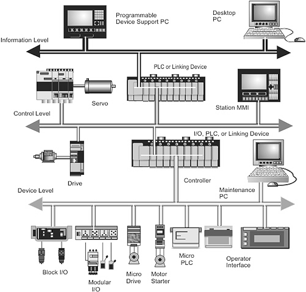
Automation system hierarchies
Interfaces between ‘levels’ as well as between different types of network at the same level require intricate data collection and application gateway techniques. The task of configuring these devices, in addition to configuring the PLCs and enterprise layer computers, provides much scope for confusion and delays. In addition to this, the need for different network hardware and maintenance techniques in the three levels complicates spares holding and technician training. In order to overcome this problem, there is a growing tendency to use a single set of networking techniques (such as Ethernet and TCP/IP), to communicate at and between all three levels.
At the enterprise layer the networking infrastructure is primarily used to transfer large units of information on an irregular basis. Examples are sending email messages, downloading web pages, making ad-hoc SQL queries, printing documents, and fetching computer programs from file servers. Deterministic and/or real-time operation is not required here.
A particular problem area is the two lower levels, where there is often an attempt to mix routine scanning of data values with on-demand signaling of alarm conditions, along with transfer of large items such as control device programs, batch reports and process recipes. There are many networks used here, such as ProfiBus (DP and FMS), FIP, Modbus Plus, DeviceNet, ControlNet and Foundation Fieldbus (H-1 and HSE). Even worse, the design characteristics of each are sufficiently different to make seamless interconnection very difficult. All these networks have their own techniques for addressing, error checking, statistics gathering, and configuration. This imposes complications even when the underlying data itself is handled in a consistent way.
One technique commonly used to offset this problem is to divide the information available at each layer into ‘domains’, and make the devices interconnecting these domains responsible for ‘translating’ requests for information. As an example, the PLC might use its device bus to scan raw input values, and then make a subset of them available as ‘data points’ on the ‘control bus’. Similarly, a cell control computer or operator station might scan data points from its various ‘control bus’ segments and make selected data available in response to queries on the ‘enterprise’ network.
Although these techniques can be made to work, they have a number of significant disadvantages:
- The intermediate gateways need to be configured to handle any data processed through them. This means that, if a PLC program is updated, it is necessary to update any related HMI or cell controller programs to reflect the changes, otherwise the information reflected to the user level will be incomplete or inconsistent. Often this must be done with little automatic support from the device vendors, who jealously guard the ‘features’ of their data items and resist the attempt to simplify their operation by conforming to standard naming and attribute conventions
- Although devices such as PLCs are designed to be extremely reliable, HMI and cell controllers are typically general-purpose computer systems, and will have a higher incidence of failures due to hardware or software problems. When such failures occur (and they will, even if care is taken in hardware design), it is important to be able to configure a replacement system and get it running as rapidly as possible. Many users today experience downtimes of many hours if a single gateway or HMI goes down, because of the difficulty in getting a replacement device to the same state as one which failed
A typical MTBF (Mean Time Between Failures) of general-purpose computer systems is 50 000 hours for hardware and 14 000 hours for software. A typical MTBF for PLC systems are 100 000 hours. At these rates, a plant with 100 PLCs or computers would expect to experience about one failure requiring hardware replacement PER MONTH. Losing a number of hours’ production each month due to hardware problems is an untenable situation. That is why automation vendors consider the ability to reinstall and restart a PLC or control system from virgin hardware in a rapid and reliable way to be mandatory.
15.3 The ‘factory of the future’
It is widely recognized that the traditional hierarchical structure of factory automation systems can be replaced with a single network, using the Internet as a model. In this model, all stations can conceivably intercommunicate and all stations can also communicate to the outside world via a firewall. Such a network would obviously be segmented for performance and security. The traditional computer-based gateways separating the three layers (enterprise, device, control) can now be replaced with off-the-shelf bridges, switches and routers with a high degree of reliability.
One of the challenges in designing such a network-based solution is the choice of a common interconnection technology. It should ideally be universal and vendor neutral and inexpensive to deploy in terms of hardware, cabling and training time. It should facilitate integration of all equipment within the plant; it should be simple to understand and configure; and it should be scalable in performance to support the future growth of the network.
Five specific areas have to be addressed in order to enable the implementation of fully open (or ‘transparent’) control systems architecture for modern day factories. They are:
- The networking protocol stack
- Application layer protocols
- Seamless access to plant-wide information
- Replacement of computer-based gateways with dedicated routers and switches
- Network access for devices
15.3.1 The networking protocol stack (OSI layers 3 and 4)
The ideal choice here is a TCP/IP. This allows integration with the Internet, enabling access to the plant on a global basis. TCP/IP is a military standard protocol suite, originally designed for end-to-end connection oriented control over long-haul networks. It is tolerant of wide speed variations and poor quality point-to-point links, and is compatible with the firewalls and proxy servers required for network security. It can operate across the Internet as well as across WANs, and is easy to troubleshoot with standard TCP/IP utilities and freeware protocol analyzers.
Considering all the advantages of TCP/IP, the overhead of 40 bytes per packet is a small price to pay.
15.3.2 Application layer protocols (OSI layer 7)
One solution for a ‘generic’ implementation of the Application layer is Modbus, a vendor neutral data representation protocol. This is the path followed by the Modbus-IDA Group in Europe and North America (see www.modbus-ida.org and www2.modbus-ida.org). Modbus has been referred to as ‘every vendor’s second choice but every integrator’s first choice’. Reasons for this include the fact that the specification is open and freely downloadable, and that the minimal implementation involves only two messages. It is easy to adapt existing serial interface software for Modbus, and also very easy to perform automatic protocol translation.
Although most implementations of the Modbus protocol are used on low-speed point-to-point serial links or twisted pair multidrop networks, it has been adapted successfully for radio, microwave, public switched telephone, infra-red, and almost any other communication mechanism conceivable. Despite the simplicity of Modbus it performs its intended function extremely well. Later in this chapter we will show how Modbus has been adapted to run over TCP.
Alternatively, vendors can modify their existing upper layer stacks to run over TCP/IP. A good example is the ODVA’s DeviceNet, which has been modified to run over TCP/IP and Ethernet and marketed under the name Ethernet/IP. The ‘IP’ or ‘Industrial Protocol” in this case refers to the Application layer protocol, namely the Control and Information Protocol or CIP. CIP has been left untouched, so the operators see no difference.
15.3.3 Seamless access to plant data
We will look at two solutions to this problem, viz. (a) the use of embedded web servers and (b) the use of OPC.
Embedded web servers
Once all computers and control devices are connected via a seamless Internet-compatible network, it becomes possible to use web servers to make plant information available to operators. This can be done in two different ways.
Firstly, a control device can incorporate its own local web server. This means that plant I/O information, accessible only by that device, can be reported in a legible form as a set of web pages, and therefore displayed on any computer on the intranet, extranet, or Internet by means of a web browser.
Alternatively, a general-purpose computer can act as a web server, and gather data for individual web page requests by generating the native Modbus requests used by the control devices. These requests can then be sent out over the Modbus/TCP network, and will interrogate either the control devices directly (if they have TCP/IP interfaces) or via simple protocol converters (such as an off-the-shelf Modbus gateway) to convert requests into a form that legacy equipment would understand.
In both cases, there are two specific obstacles, namely that of reconfiguring a computer that has replaced a defective one, and maintaining the data directory.
In order to solve the problem of reconfiguring a computer after replacing a defective one, a network computer can be used as a web server, which means that the latter would be self-configuring on installation. The network computers then install themselves from a server elsewhere on the network when powered up. This means that if a network computer were ever to fail, a new computer could be installed in its place, powered up, and it would immediately take on the same identity as its predecessor.
Another problem is how to present and maintain the directory that stores and maintains the attributes of all data items. Despite a variety of proprietary solutions to this problem, there is an emerging standard called LDAP (Lightweight Directory Access Protocol), which was originally intended for keeping a registry of email addresses for an organization. Under this scheme, LDAP would maintain a hierarchical ‘picture’ of plant points within machines, machines within locations, and areas within an organization. LDAP makes it easy to reorganize the directory if the organization of the physical machines and data points needs to be modified.
Each plant point could have attributes such as tag name, data type, scale, input limits, units, reference number, size, orientation and physical machine name. In addition to this, each physical machine would have attributes such as IP address and MAC address.
OPC
Another solution gaining popularity is OPC. Many modern SCADA systems are built entirely around OPC, and systems such as ProfiNet are inherently OPC compatible.
OPC was originally designed around Microsoft DCOM, although several vendors have implemented their own version of DCOM. COM is Microsoft’s Component Object Model and DCOM is the distributed version thereof, i.e. DCOM objects can reside on different processors, even on a LAN or a WAN. This is a component software architecture that can be used to build software components (black boxes) that can interoperate regardless of where they are situated. DCOM also provides the mechanisms for the communication between these components, shared memory management between them, and the dynamic loading of components if and when required. These objects are written in an object oriented language such as C++ or VB and have software interfaces that can be used to access their functions (or methods as they are called). Interfaces are generally given names starting with an uppercase ‘I’ such as IOPCShutdown. Each object and each interface is considered unique and is given a 128-bit ‘GUID’ (Globally Unique ID) number to identify it.
DCOM, in turn, typically uses a TCP/IP stack with RPC (Remote Procedure Call) in the Application layer for communication between OPC clients and servers across a network.
OPC initially stood for OLE (Object Linking and Embedding) for Process Control. In the meantime OLE has been replaced with ActiveX, but the initialism ‘OPC’ remains. OPC is an open, standard software infrastructure for the exchange of process data. It specifies a set of software interfaces and logical objects as well as the functions (methods) of those objects. Vendors and users can develop their own clients and servers if they wish, with or without programming knowledge. The main reason for the existence of OPC is the need to access process control information regardless of the operating system or hardware involved. In other words, OPC data is accessed in a consistent way regardless of who the vendor of the system is. OPC is built around the client-server concept where the server collects plant data and passes it on to a client for display.
Since OPC was designed around Microsoft DCOM it was initially limited to Windows operating systems. Despite its legacy, DCOM is currently implemented on all major operating systems as well as several imbedded real-time operating systems and is therefore effectively vendor neutral. In fact, much of the non-real-time PROFInet communication is built on DCOM.
OPC effectively creates a ‘software bus’ allowing multiple clients to access data from multiple servers without the need for any special drivers.

The concept of a ‘software bus’
The following figure shows an application (a client, for example) obtaining plant data from an OPC server. The OPC server, in turn, obtains its information from some physical I/O or by virtue of a bridging process from a SCADA system which, in turn, gathers physical plant information through some physical I/O.

Relationship between OPC client and OPC server
There are several OP specifications. The most common one is OPC DA (Data Access). This standard defines a set of application interfaces, allowing software developers to develop clients that retrieve data from a server. Through the client, the user can locate individual OPC servers and perform simple browsing in the name spaces (i.e. all the available tags) of the OPC server.
Although OPC DA allows a client to write back data to the server, it is primarily intended to read data from the server and hence to create a ‘window’ into the plant.
Another emerging OPC standard is OPC DX (Data Exchange). OPC DX is an extension of the OPC DA specification and defines a communication standard for the higher-level exchange of non-time-critical user data at system levels between different makes of control systems, e.g. between Foundation Fieldbus HSE, Ethernet/IP and PROFInet.
OPC DX allows system integrators to configure controllers from different vendors through a standard browser interface without any regard for the manufacturer of a specific node. In other words, it allows a common view of all devices.

Using OPC DX between various systems
15.3.4 Routers and switches
The advantage of using Ethernet at all levels in the enterprise is that these levels can then be interlinked by means of standard off-the-shelf Ethernet compatible products such as routers and switches.
Switches
The use of switching hubs is the key to high performance coupling between the different plant network layers since it becomes easy to mix stations of different speeds. Inserting switches between sub-networks requires no change to hardware or software and effectively isolates the traffic on the two network layers joined by it (i.e. the traffic on the subnets connected via the switch does not ‘leak’ across the switch). In order to preserve bandwidth, it is imperative not to use broadcast techniques.
Routers
In terms of inter-layer connection, routers can augment the speed adaptation function by being deployed in series with a switching hub. A throttling router, connected in series with the switch, can impose delays in order to achieve flow control in a situation where the destination network cannot cope with the data flow. Routers also assist in implementing security measures, such as Access Control Lists (ACLs). They can even be combined with firewalls for added security.
15.3.5 Network access for devices (OSI layers 1 and 2)
Ethernet is becoming the de facto standard for the implementation of the Physical and Data Link layers of the OSI model because of its scalability and relatively low cost. The following paragraphs will briefly deal with the factors that, until recently, have been Ethernet shortcomings namely throughput, determinism and redundancy.
Throughput concerns
The entry-level IEEE 802.3 Ethernet standard used to be 10BaseT but this can almost be regarded as a legacy technology; so the trend is to use Fast Ethernet (100BaseX) in industrial environments. In theory one could even deploy Gigabit Ethernet (1000BaseX), but IP67 rated connectors to accommodate this speed is still a problem. For the enterprise level, 10 Gigabit Ethernet can be used.
Determinism (response time)
Initially Ethernet (the 10 Mbps versions) operated in half-duplex mode with contention (CSMA/CD) as a medium access control mechanism. Consequently it has been argued that Ethernet does not possess sufficient determinism. This problem was solved to some extent by switches, full duplex operation, and IEEE 802.1p ‘traffic class expediting’ or ‘message prioritization’, which allows the delivery of time-critical messages in a deterministic fashion. Initially designed for multimedia applications, it directly impacts on Ethernet as a control network by allowing system designers to prioritize messages, guaranteeing the delivery of time critical data with deterministic response times. This ability has been used to produce Ethernet systems that typically provide a deterministic scan time in the 2 to 3 millisecond range for one I/O rack with 128 points.
For motor control applications this is still not good enough; hence there are several vendors marketing Ethernet ‘field buses’ that employ the IEEE 1588 clock synchronization standard and are capable of scanning in excess of a thousand I/O points per millisecond, and can synchronize servo axes with accuracies in the microsecond region. Examples are Sercos III, EtherCat and ProfiNet RT.
Redundancy
The older IEEE 802.1d ‘Spanning Tree Protocol’ (STP) provided the ability to add redundant links to a network device such as a bridge or switch. This facilitates automatic recovery of network connectivity when there is a link or component failure anywhere in the network path. This standard obviates the need for custom solutions when redundancy is required as part of the control solution, and allows Ethernet switches to be wired into rings for redundancy purposes. Redundant or even dual-redundant switched Ethernet rings are now commonplace. What’s more, these switches can be interconnected with fiber links of up to 120 km for certain brands.
Unfortunately STP was too slow (30-60 seconds needed for reconfiguration) for Industrial applications. As a result, several vendors including Cisco, Siemens and Hirschmann developed their own versions of, or enhancements to, STP. The newer IEEE 802.1W ‘Rapid Spanning Tree Protocol’ (RSTP) can reconfigure itself in less than 10 seconds if it detects a failure in the redundant system.
15.3.6 Thin servers
Universal thin servers
A universal thin server is an appliance that network-enables any serial device such as a printer or weighbridge that has an RS-232 port. In addition to the operating system and protocol independence of general thin servers, a universal thin server is application- independent by virtue of its ability to network any serial device.
The universal thin server is a product developed primarily for environments in which machinery, instruments, sensors and other discrete ‘devices’ generate data that was previously inaccessible through enterprise networks. They allow nearly any device to be connected, managed and controlled over a network or the Internet.
Thin server applications
In general, thin servers can be used for data acquisition, factory floor automation, security systems, scanning devices and medical devices.
An interesting thin server application regulates cattle feed in stock yards. Cattle wear radio frequency ID tags in their ears that relay data over a TCP/IP network as they step on to a scale. By the time the cattle put their heads in a trough to eat, the system has distributed the proper mix of feed.
Thin servers control video cameras used to monitor highway traffic. The US Border Patrol uses similar cameras to spot illegal border crossings. Food processing companies use the technology to track inventory in a warehouse, or the weight of consumable items rolling off an assembly line.
15.3.7 Network capable application processors (NCAPs)
The IEEE 1451 activities comprise two parts, each managed by its own working group. IEEE 1451.1 targets the interface between the smart device and the network, while 1451.2 focuses on the interface between the sensor/transducer and the on-board microprocessor within the smart device.
IEEE 1451.1 defines a ‘Network Capable Application Processor (NCAP) Information Model’ that allows smart sensors and actuators to interface with many networks including Ethernet. The standard strives to achieve this goal by means of a common network object model and use of a standard API, but it specifically does not define device algorithms or message content.
IEEE 1451.2 is concerned with transducer-to-microprocessor communication protocols and transducer ‘Electronic Data Sheet’ formats. This standard provides an interface that sensor and actuator suppliers can use to connect transducers to microprocessors within their smart device without worrying about what kind of microprocessor is on-board. A second part of the P1451.2 activity is the specification of Electronic Data Sheets and their formats. These data sheets, which amount to physically placing the device descriptions inside the smart sensor, provide a standard means for describing smart devices to other systems. These Transducer Electronic Data Sheets (TEDS) also allow self-identification of the device on the network.
15.4 Modbus/TCP
15.4.1 Introduction
The Modbus Messaging protocol is an Application layer (OSI layer 7) protocol that provides communication between devices connected to different types of buses or networks. It implements a client/server architecture and operates essentially in a ‘request/response’ mode, irrespective of the media access control method used at layer 2. The client (on the controller) issues a request; the server (on the target device) then performs the required action and initiates a response.

Modbus transaction
The Modbus Messaging protocol needs additional support at the lower layers and in the case of Modbus Serial implementations a master/slave (half-duplex) layer 2 protocol transmits the data in asynchronous mode over RS-232, RS-485 or Bell 202 type modem links. Alternatively, HDLC (a token passing layer 2 protocol) transmits data in synchronous mode over RS-485 for Modbus Plus. This section illustrates the TCP/IP/Ethernet approach, which enables client/server interaction over routed networks albeit at the cost of additional overheads such as processing time and more headers.
In order to match the Modbus Messaging protocol to TCP, an additional sub-layer is required. The function of this sub-layer is to encapsulate the Modbus PDU so that it can be transported as a packet of data by TCP/IP (see Figure 15.6). Strictly speaking this should have been called an APDU (Application Protocol Data Unit) but we will stick with the Modbus designation.

Modbus/TCP communication stack
15.4.2 Modbus encapsulation
One might well ask why connection-oriented TCP is used, rather than the datagram-oriented UDP. TCP has more overheads, and as a result it is slower than UDP. The main reason for this choice is to keep control of individual ‘transactions’ by enclosing them in connections that can be identified, supervised, and canceled without requiring specific action on the part of the client or server applications. This gives the mechanism a wide tolerance to network performance changes, and allows security features such as firewalls and proxies to be easily added.
The PDU consisting of data and function code is encapsulated by adding a ‘Modbus on TCP Application Protocol’ (MBAP) header in front of the PDU. The resulting Modbus/TCP ADU, consisting of the PDU plus MBAP header, is then transported as a chunk of data via TCP/IP and Ethernet. Once again, this should have been called a TADU (Transport Application Data Unit) but we will use the Modbus designation.
Whereas Modbus Serial forms the ADU by simply appending a 1-bit unit identifier to the PDU, the MBAP header is much larger, although it still contains the 1-byte unit identifier (‘slave address’) for communicating with serial devices. A byte count is included so that in the case of long messages being split up by TCP, the recipient is kept informed of the exact number of bytes transmitted. The ADU no longer contains a checksum (as in the serial implementation), as this function is performed by TCP.
| Fields | Length | Description | Client | Server |
|---|---|---|---|---|
| Transaction Identifier | 2 Bytes | Identification of a Modbus Request/ Response transaction | Initialized by the client | Recopied by the server from the received request |
| Protocol Identifier | 2 Bytes | 0 = Modbus protocol | Initialized by the client | Recopied by the server from the received request |
| Length | 2 Bytes | Number of following bytes | Initialized by the client (request) | Initialized by the server (response) |
| Unit Identifier | 1 Byte | Identification of a remote device (slave) connected on a serial line or on other buses | Initialized by the client | Recopied by the server from the received request |
Table 15.1
MBAP fieldsThe MBAP header is 7 bytes long and comprises the following 4 fields (see Table 15/.1):
- The Transaction Identifier is a pseudo-random number used for pairing requests and responses. The Modbus server simply copies this number received in the request from the client back into the response to the client.
- The Protocol Identifier is used for multiplexing between systems. The Modbus protocol is defined as value 0.
- The Length field is a byte count of all the fields following it, including the Unit Identifier and data fields.
- The Unit Identifier (slave address) is used for routing between systems, typically to a Modbus or Modbus Plus target device through a gateway between the serial line and a TCP/IP network. The client sets it and the server must return the same value.
The Modbus/TCP ADU is therefore constructed as follows:
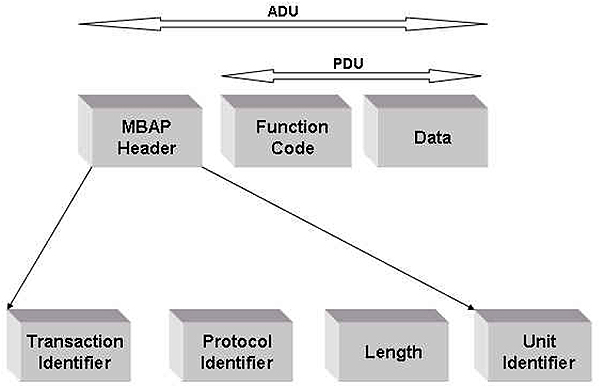
Modbus/TCP ADU
All Modbus/TCP ADUs are sent via registered port 502 and the fields are encoded big-endian, which means that if a number is represented by more than one byte, the most significant byte is sent first. TCP/IP transports the entire Modbus ADU as data (as shown in the following figure).

Transportation of Modbus ADU
15.5 Ethernet/IP (Ethernet/Industrial Protocol)
15.5.1 Introduction
DeviceNet™ and ControlNet™ are two well-known industrial networks based on CIP, the Control and Information Protocol. Both networks have been developed by Rockwell Automation, but are now owned and maintained by the two manufacturers’ organizations viz. ODVA (Open DeviceNet Vendors Association) and CI (ControlNet International). ODVA and CI have recently introduced the newest member of this family viz. EtherNet/IP. This section describes the techniques and mechanisms that are used to implement Ethernet/IP and will attempt to give an overall view of the system, taking into account the fact that layers 1 thru 4 of the OSI model (the bottom three layers of the TCP model) have already been dealt with earlier in this manual.
15.5.2 Ethernet/IP vs. DeviceNet and ControlNet
Ethernet/IP is an open industrial network standard based on Ethernet, using commercial off-the-shelf (COTS) technology and TCP/IP. It allows users to collect, configure and control data, and provides interoperability between equipment from various vendors, of which there are several hundred already.
The system is defined in terms of several open standards, which have a wide level of acceptance. They are Ethernet (IEEE802.3), TCP/IP, and CIP (Control Information Protocol, EN50170 and IEC 61158).
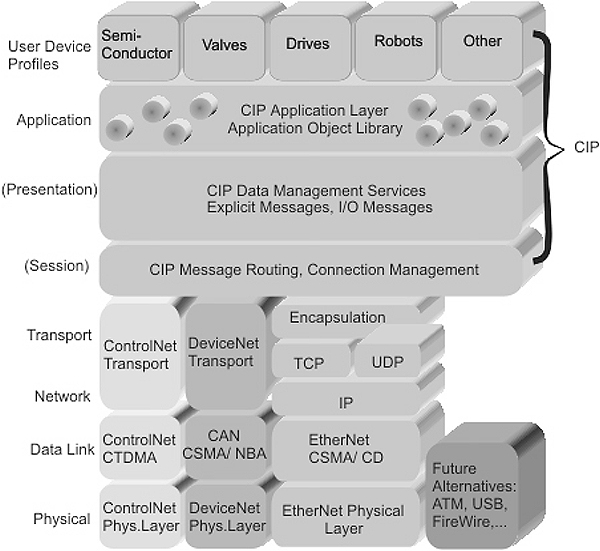
Ethernet/IP, DeviceNet and ControlNet stacks
As Figure 15.9 shows, CIP has already been in use with DeviceNet and ControlNet, the only difference between those two systems being the implementation of the four bottom layers. Now TCP/IP has been added as an alternative network layer/transport layer, but CIP remains intact.
TCP is typically used to download ladder programs between a workstation and a PLC, for MMI software that reads or writes PLC data tables, or for peer-to-peer messaging between two PLCs. This type of communication is referred to as ‘explicit’ communication.
Through TCP, Ethernet/IP is able to send explicit (connection oriented) messages, in which the data field carries both protocol information and instructions. Here, nodes must interpret each message, execute the requested task, and generate responses. These types of messages are used for device configuration and various diagnostics.
UDP is typically used for network management functions, applications that do not require reliable data transmission, applications that are willing to implement their own reliability scheme, such a flash memory programming of network devices, and for input/output (I/O) operations.
For connectionless real-time messaging, multicasting, and for sending implicit messages, Ethernet/IP uses UDP. Implicit messages contain no protocol information in the data field, only real-time I/O data. The meaning of the data is predefined in advance; therefore processing time in the node during runtime is reduced. Because these messages are low on overhead and short, they can pass quickly enough to be useful for certain time-critical control applications.
Between TCP/UDP and CIP is an encapsulating protocol, which appends its own encapsulating header and checksum to the CIP data to be sent before passing it on to TCP or UDP. In this way the CIP information is simply passed on by TCP/IP or UDP/IP as if it is a chunk of data.

Explicit vs. implicit messaging
As shown in Figure 15.9, CIP covers not only layers 5, 6 and 7 of the OSI model, but also the ‘User layer’ (layer 8), which includes the user device profiles. Apart from the common device profiles, CIP also includes the common object library, the common control services and the common routing services. The OSI model has no layer 8, but items such as device profiles do not fit within the conceptual structure of the OSI model, hence vendors often add a ‘layer 8’ above layer 7 for this purpose.
CIP co-exists with the other TCP/IP application layer protocols as shown in Figure 15.11.

CIP vs. other Application layer protocols
16.1 Introduction
This section addresses common faults on Ethernet networks. Ethernet encompasses layers 1 and 2, namely the Physical and Data Link layers of the OSI model. This is equivalent to the bottom layer (the Network Interface layer) in the ARPA (DoD) model. This section will focus on those layers only, as well as on the actual medium over which the communication takes place.
16.2 Common problems and faults
Ethernet hardware is fairly simple and robust, and once a network has been commissioned, providing the cabling has been done professionally and certified, the network should be fairly trouble-free.
Most problems will be experienced at the commissioning phase, and could theoretically be attributed to the cabling, the LAN devices (such as hubs and switches), the NICs or the protocol stack configuration on the hosts.
The wiring system should be installed and commissioned by a certified installer (the suppliers of high-speed Ethernet cabling systems, such as ITT, will not guarantee their wiring if not installed by a certified installer). This effectively rules out wiring problems for new installations.
If the LAN devices such as hubs and switches are from reputable vendors, it is highly unlikely that they will malfunction in the beginning. Care should nevertheless be taken to ensure that intelligent (managed) hubs and switches are correctly set up.
The same applies to NICs. NICs rarely fail and nine times out of ten the problem lies with a faulty setup or incorrect driver installation, or an incorrect configuration of the higher level protocols such as IP.
16.3 Tools of the trade
Apart from a fundamental understanding of the technologies involved, sufficient time, a pair of eyes, patience, and many cups of coffee or tea, the following tools are helpful in isolating Ethernet-related problems.
16.3.1 Multimeters
A simple multimeter can be used to check for continuity and cable resistance, as will be explained in this section.
16.3.2 Handheld cable testers
There are many versions on the market, ranging from simple devices that basically check for wiring continuity to sophisticated devices that comply with all the prerequisites for 1000Base–T wiring infrastructure tests. Testers are available from several vendors such as MicroTest, Fluke, and Scope.

OMNIscanner cable tester
16.3.3 Fiber optic cable testers
Fiber optic testers are simpler than UDP testers, since they basically only have to measure continuity and attenuation loss. Some UDP testers can be turned into fiber optic testers by purchasing an attachment that fits onto the existing tester. For more complex problems such as finding the location of a damaged section on a fiber optic cable, an alternative is to use a proper Optical Time Domain Reflectometer (OTDR) but these are expensive instruments and it is often cheaper to employ the services of a professional wiring installer (with his own OTDR) if this is required.
16.3.4 Traffic generators
A traffic generator is a device that can generate a pre-programmed data pattern on the network. Although they are not strictly speaking used for fault finding, they can be used to predict network behavior due to increased traffic, for example, when planning network changes or upgrades. Traffic generators can be stand-alone devices or they can be integrated into hardware LAN analyzers such as the Hewlett Packard 3217.
16.3.5 RMON probes
An RMON (Remote MONitoring) probe is a device that can examine a network at a given point and keep track of captured information at a detailed level. The advantage of a RMON probe is that it can monitor a network at a remote location. The data captured by the RMON probe can then be uploaded and remotely displayed by the appropriate RMON management software. RMON probes and the associated management software are available from several vendors such as 3COM, Bay Networks and NetScout. It is also possible to create an RMON probe by running commercially available RMON software on a normal PC, although the data collection capability will not be as good as that of a dedicated RMON probe.
16.3.6 Handheld frame analyzers
Handheld frame analyzers are manufactured by several vendors such as Fluke, Scope, Finisar and PsiberNet, for up to Gigabit Ethernet speeds. These devices can perform link testing, traffic statistics gathering etc. and can even break down frames by protocol type. The drawback of these testers is the small display and the lack of memory, which results in a lack of historical or logging functions on these devices.
An interesting feature of some probes is that they are non-intrusive, i.e. they simply clamp on to the wire and do not have to be attached to a hub or switch port.

Clamp-on gigabit Ethernet probe
16.3.7 Software protocol analyzers
Software protocol analyzers are software packages that run on PCs and use either a general purpose or a specialized NIC to capture frames from the network. The NIC is controlled by a so-called promiscuous driver, which enables the NIC to capture all packets on the medium and not only those addressed to it in broadcast or unicast mode.
There are excellent freeware protocol analyzers such as Ethereal or Analyzer, the latter being developed at the Polytechnic of Torino in Italy. Top of the range software products such as Network Associates’ Sniffer or WaveTek Wandel Goltemann’s Domino Suite have sophisticated expert systems that can aid in the analysis of the captured software, but unfortunately this comes at a price.
16.3.8 Hardware based protocol analyzers
Several manufacturers such as Hewlett Packard, Network Associates and WaveTek Wandel & Goltemann also supply hardware based protocol analyzers using their protocol analysis software running on a proprietary hardware infrastructure. This makes them very expensive but dramatically increases the power of the analyzer. For fast and gigabit Ethernet, this is probably the better approach. As a compromise one could use their software on a PC, but with a specially supplied NIC. The advantage of a hardware-based approach is that one can capture packets at level 1 of the OSI model. A software-based analyzer can only capture packets once they have been read by the NIC, and can therefore not capture malformed packets
16.4 Problems and solutions
16.4.1 Noise
If excessive noise is suspected on a coax or UTP cable, an oscilloscope can be connected between the signal conductor(s) and ground. This method will show up noise on the conductor, but will not necessarily give a true indication of the amount of power in the noise. A simple and cheap method to pick up noise on the wire is to connect a small loudspeaker between the conductor and ground. An operational amplifier can be used as an input buffer, so as not to ‘load’ the wire under observation. The noise will be heard as an audible signal.
The quickest way to get rid of a noise problem, apart from using screened UTP (ScTP), is to change to a fiber-based instead of a copper-based network, for example, by using 100Base–FX instead of 100Base-TX.
Noise can to some extent be counteracted on a coax-based network by earthing the screen AT ONE END ONLY. Earthing it on both sides will create an earth loop. This is normally accomplished by means of an earthing chain or an earthing screw on one of the terminators. Care should also be taken not to allow contact between any of the other connectors on the segment and ground.
16.4.2 Thin coax problems
Incorrect cable type
This is still used in some legacy systems. The correct cable for thin Ethernet is RG58-A/U or RG-58C/U. This is a 5 mm diameter coaxial cable with 50 ohm characteristic impedance and a stranded center conductor. Incorrect cable used in a thin Ethernet system can cause reflections, resulting in CRC errors, and hence many retransmitted frames.
The characteristic impedance of coaxial cable is a function of the ratio between the center conductor diameter and the screen diameter. Hence other types of coax may closely resemble RG-58, but may have different characteristic impedance.
Loose connectors
The BNC coaxial connectors used on RG-58 should be of the correct diameter, and should be properly crimped onto the cable. An incorrect size connector or a poor crimp could lead to intermittent contact problems, which are very hard to locate. Even worse is the ‘Radio Shack’ hobbyist type screw-on BNC connector that can be used to quickly make up a cable without the use of a crimping tool. These more often than not lead to very poor connections. A good test is to grip the cable in one hand, and the connector in another, and pull very hard. If the connector comes off, the connector mounting procedures need to be seriously reviewed.
Excessive number of connectors
The total length of a thin Ethernet segment is 185 m and the total number of stations on the segment should not exceed 30. However, each station involves a BNC T-piece plus two coax connectors and there could be additional BNC barrel connectors joining the cable. Although the resistance of each BNC connector is small, they are still finite and can add up. The total resistance of the segment (cable plus connectors) should not exceed 10 ohms otherwise problems can surface.
An easy method of checking the loop resistance (the resistance to the other end of the cable and back) is to remove the terminator on one end of the cable and measure the resistance between the connector body and the center contact. The total resistance equals the resistance of the cable plus connectors plus the terminator on the far side. This should be between 50 and 60 ohms. Anything more than this is indicative of a problem.
Overlong cable segments
The maximum length of a thin net segment is 185 m. This constraint is not imposed by collision domain considerations, but rather by the attenuation characteristics of the cable. If it is suspected that the cable is too long, its length should be confirmed. Usually, the cable is within a cable trench and hence it cannot be visually measured. In this case, a TDR can be used to confirm its length.
Stub cables
For thin Ethernet (10Base2), the maximum distance between the bus and the transceiver electronics is 4 cm. In practice, this is taken up by the physical connector plus the PC board tracks leading to the transceiver, which means that there is no scope for a drop cable or ‘stub’ between the NIC and the bus. The BNC T-piece has to be mounted directly on to the NIC.
Users do occasionally get away with putting a short stub between the T-piece and the NIC, but this invariably leads to problems in the long run.
Incorrect terminations
10Base2 is designed around 50-ohm coax and hence requires a 50-ohm terminator at each end. Without the terminators in place, there would be so many reflections from each end that the network would collapse. A slightly incorrect terminator is better than no terminator, yet may still create reflections of such magnitude that it affects the operation of the network.
A 93-ohm terminator looks no different than a 50-ohm terminator; therefore it should not be automatically assumed that a terminator is of the correct value.
If two 10Base2 segments are joined with a repeater, the internal termination on the repeater can be mistakenly left enabled. This leads to three terminators on the segment, creating reflections and hence affecting the network performance.
The easiest way to check for proper termination is by alternatively removing the terminators at each end, and measuring the resistance between connector body and center pin. In each case, the result should be 50 to 60 ohms. Alternatively, one of the T-pieces in the middle of the segment can be removed from its NIC and the resistance between the connector body and the center pin measured. The result should be the value of the two half cable segments (including terminators) in parallel, i.e. 25 to 30 ohms.
Invisible insulation damage
If the internal insulation of coax is inadvertently damaged, for example, by placing a heavy point load on the cable, the outer cover could return to its original shape whilst leaving the internal dielectric deformed. This leads to a change of characteristic impedance at the damaged point resulting in reflections. This, in turn, could lead to standing waves being formed on the cable.
An indication of this problem is when a work station experiences problems when attached to a specific point on a cable, yet functions normally when moved a few meters to either side. The only solution is to remove the offending section of the cable. Because of the nature of the damage, it cannot be seen by the naked eye and the position of the damage has to be located with a TDR. Alternatively, the whole cable segment has to be replaced.
Invisible cable break
This problem is similar to the previous one, with the difference that the conductor has been completely severed at a specific point. Despite the terminators at both ends of the cable, the cable break effectively creates two half segments, each with an un-terminated end, and hence nothing will work.
Often the only way to discover the location of the break is by using a TDR.
16.4.3 Thick coax problems
Thick coax (RG-8), as used for 10Base5 or thick Ethernet, will basically exhibit the same problems as thin coax yet there are a few additional complications.
Loose connectors
10Base5 uses N-type male screw-on connectors on the cable. As with BNC connectors, incorrect procedures or a wrong sized crimping tool can cause sloppy joints. This can lead to intermittent problems that are difficult to locate.
Again, a good test is to grab hold of the connector and to try and rip it off the cable with brute force. If the connector comes off, it was not properly installed in the first place.
Dirty taps
The MAU transceiver is often installed on a thick coax by using a vampire tap, which necessitates pre-drilling into the cable in order to allow the center pin of the tap to contact the center conductor of the coax. The hole has to go through two layers of braided screen and two layers of foil. If the hole is not properly cleaned, pieces of the foil and braid can remain and cause short circuits between the signal conductor and ground.
Open tap holes
When a transceiver is removed from a location on the cable, the abandoned hole should be sealed. If not, dirt or water could enter the hole and create problems in the long run.
Tight cable bends
The bend radius on a thick coax cable may not exceed 10 inches. If it does, the insulation can deform to such an extent that reflections are created leading to CRC errors. Excessive cable bends can be detected with a TDR.
Excessive loop resistance
The resistance of a cable segment may not exceed 5 ohms. As in the case of thin coax, the easiest way to do this is to remove a terminator at one end and measure the loop resistance. It should be in a range of 50–55 ohms.
16.4.4 UTP problems
The most commonly used tool for UTP troubleshooting is a cable meter or pair scanner. At the bottom end of the scale, a cable tester can be an inexpensive tool, only able to check for the presence of wire on the appropriate pins of a RJ-45 connector. High-end cable testers can also test for noise on the cable, cable length, and crosstalk (such as near end signal crosstalk or NEXT) at various frequencies. It can check the cable against CAT5/5e specifications and can download cable test reports to a PC for subsequent evaluation.
The following is a description of some wiring practices that can lead to problems.
Incorrect wire type (solid/stranded)
Patch cords must be made with stranded wire. Solid wire will eventually suffer from metal fatigue and crack right at the RJ-45 connector, leading to permanent or intermittent open connections. Some RJ-45 plugs, designed for stranded wire, will actually cut through the solid conductor during installation, leading to an immediate open connection. This can lead to CRC errors resulting in slow network performance, or can even disable a workstation permanently. The length of the patch cords or flyleads on either end of the link may not exceed 5m, and these cables must be made from stranded wire.
The permanently installed cable between hub and workstation, on the other hand, should not exceed 90m and must be of the solid variety. Not only is stranded wire more expensive for this application, but the capacitance is higher, which may lead to a degradation of performance.
Incorrect wire system components
The performance of the wire link between a hub and a workstation is not only dependent on the grade of wire used, but also on the associated components such as patch panels, Surface Mount Units (SMUs) and RJ-45 type connectors. A single substandard connector on a wire link is sufficient to degrade the performance of the entire link.
High quality Fast and Gigabit Ethernet wiring systems use high-grade RJ-45 connectors that are visibly different from standard RJ-45 type connectors.
Incorrect cable type
Care must be taken to ensure that the existing UTP wiring is of the correct category for the type of Ethernet being used. For 10BaseT, Cat3 UTP is sufficient, while Fast Ethernet (100Base-TX) requires Cat5 and Gigabit Ethernet requires Cat5e or better. This applies to patch cords as well as the permanently installed (‘infrastructure’) wiring.
Most industrial Ethernet systems nowadays are 100Base-X-based and hence they use Cat5 wiring. For such applications it might be prudent to install screened Cat5 wiring (ScTP) for better noise immunity. ScTP is available with a common foil screen around the 4 pairs or with an individual foil screen around each pair. Better still is Cat5i wiring which has only two wire pairs of a thicker gauge, as well as a braided shield.
A common mistake is to use telephone grade patch (‘silver satin’) cable for the connection between an RJ-45 wall socket (SMU) and the NIC. Telephone patch cables use very thin wires that are untwisted, leading to high signal loss and large amounts of crosstalk. This will lead to signal errors causing retransmission of lost packets, which will eventually slow the network down.
‘Straight’ vs. crossover cable
A 10BaseT or 100Base-TX patch cable consists of 4 wires (two pairs) with an RJ-45 connector at each end. The pins used for the TX and RX signals are typically 1, 2 and 3, 6. Although a typical patch cord has 8 wires (4 pairs), the 4 unused wires are nevertheless crimped into the connector for mechanical strength. In order to facilitate communication between computer and hub, the TX and RX ports on the hub are reversed, so that the TX on the computer and the RX on the hub are interconnected whilst the TX on the hub is connected to the RX on the hub. This requires a ‘straight’ interconnection cable with pin 1 wired to pin 1, pin 2 wired to pin 2, etc.
If the NICs on two computers are to be interconnected without the benefit of a hub, a normal straight cable cannot be used since it will connect TX to TX and RX to RX. For this purpose, a crossover cable has to be used, in the same way as a ‘null’ modem cable. Crossover cables are normally color coded (for example, green or yellow) in order to differentiate them from straight cables.
A crossover cable can create problems when it looks like a normal straight cable and the unsuspecting person uses it to connect a NIC to a hub or a wall outlet. A quick way to identify a crossover cable is to hold the two RJ-45 connectors side by side and observe the colors of the 8 wires in the cable through the clear plastic of the connector body. The sequence of the colors should be the same for both connectors.
Hydra cables
Some 10BaseT hubs feature 50 pin connectors to conserve space on the hub. Alternatively, some building wire systems use 50 pin connectors on the wiring panels but the hub equipment has RJ-45 connectors. In some cases, hydra or octopus cable has to be used. This consists of a 50 pin connector connected to a length of 25-pair cable, which is then broken out as a set of 12 small cables, each with an RJ-45 connector. Depending on the vendor the 50-pin connector can be attached through locking clips, Velcro strips or screws. It does not always lock down properly, although at a glance it may seem so. This can cause a permanent or intermittent break of contact on some ports.
For 10BaseT systems, near end crosstalk (NEXT), which occurs when a signal is coupled from a transmitting wire pair to a receiving wire pair close to the transmitter, (where the signal is strongest) causes most problems. On a single 4 pair cable, this is not a serious problem, as only two pairs are used but on the 25 pair cable, with many signals in close proximity, this can create problems. This can be very difficult to troubleshoot since it will require test equipment that can transmit on all pairs simultaneously.
Excessive untwists
On Cat5 cable, crosstalk is minimized by twisting each cable pair. However, in order to attach a connector at the end the cable has to be untwisted slightly. Great care has to be taken since excessive untwists (more than 1 cm) is enough to create excessive crosstalk, which can lead to signal errors. This problem can be detected with a high quality cable tester.
Stubs
A stub cable is an abandoned telephone cable leading from a punch-down block to some other point. This does not create a problem for telephone systems, but if the same Cat3 telephone cabling is used to support 10BaseT, then the stub cables may cause signal reflections that result in bit errors. Again, a high quality cable tester only will be able to detect this problem.
Damaged RJ-45 connectors
On RJ-45 connectors without protective boots, the retaining clip can easily break off especially on cheaper connectors made of brittle plastic. The connector will still mate with the receptacle but will retract with the least amount of pull on the cable, thereby breaking contact. This problem can be checked by alternatively pushing and pulling on the connector and observing the LED on the hub, media coupler or NIC where the suspect connector is inserted. Because of the mechanical deficiencies of ‘standard’ RJ-45 connectors they are not commonly used on Industrial Ethernet systems.
16.4.5 Fiber optic problems
Since fiber does not suffer from noise, interference and crosstalk problems, there are basically only two issues to contend with namely attenuation and continuity.
The simplest way of checking a link is to plug each end of the cable into a fiber hub, NIC or fiber optic transceiver. If the cable is OK, the LEDs at each end will light up. Another way of checking continuity is by using an inexpensive fiber optic cable tester consisting of a light source and a light meter to test the segment.
More sophisticated tests can be done with an OTDR. OTDRs not only measure losses across a fiber link, but can also determine the nature and location of the losses. Unfortunately, they are very expensive but most professional cable installers will own one.
10BaseFX and 100Base-FX use LED transmitters that are not harmful to the eyes, but Gigabit Ethernet uses laser devices that can damage the retina of the eye. It is therefore dangerous to try and stare into the fiber (all systems are infrared and therefore invisible anyway!).
Incorrect connector installation
Fiber optic connectors can propagate light even if the two connector ends are not touching each other. Eventually, the gap between the fiber ends may be so far apart that the link stops working. It is therefore imperative to ensure that the connectors are properly latched.
Dirty cable ends
Because of the small fiber diameter (8.5–62.5 microns) and the low light intensity, a speck of dust or some finger oil deposited by touching the connector end is sufficient to affect communication. For this reason, dust caps must be left in place when the cable is not in use and a fiber optic cleaning pad must be used to remove dirt and oils from the connector point before installation.
Component aging
The amount of power that a fiber optic transmitter can radiate diminishes during the working life of the transmitter. This is taken into account during the design of the link but in the case of a marginal design, the link could start failing intermittently towards the end of the design life of the equipment. A fiber optic power meter can be used to confirm the actual amount of loss across the link but an easy way to troubleshoot the link is to replace the transceivers at both ends of the link with new ones.
16.4.6 AUI problems
Excessive cable length
The maximum length of the AUI cable is 50m but this assumes that the cable is a proper IEEE 802.3 cable. Some installations use lightweight office grade cables that are limited to 12m in length. If these cables are too long, the excessive attenuation can lead to intermittent problems.
DIX latches
The DIX version of the 15 pin D-connector uses a sliding latch. Unfortunately, not all vendors adhered to the IEEE 802 specifications and some used lightweight latch hardware which resulted in a connector that can very easily become unstuck. There are basically two solutions to the problem. The first solution is to use a lightweight (office grade) AUI cable, providing that distance is not a problem. This places less stress on the connector. The second solution is to use a special plastic retainer such as the ‘ET Lock’ made specifically for this purpose.
SQE test
The Signal Quality Error (SQE) test signal is used on all AUI based equipment to test the collision circuitry. This method is only used on the old 15 pin AUI based external transceivers (MAUs) and sends a short signal burst (about 10 bit times in length) to the NIC just after each frame transmission. This tests both the collision detection circuitry and the signal paths. The SQE operation can be observed by means of an LED on the MAU.
The SQE signal is only sent from the transceiver to the NIC and not on to the network itself. It does not delay frame transmissions but occurs during the inter-frame gap and is not interpreted as a collision.
The SQE test signal must, however, be disabled if an external transceiver (MAU) is attached to a repeater. If this is not done the repeater will detect the SQE signal as a collision and will issue a jam signal. As this happens after each packet, it can seriously delay transmissions over the network. The problem is that it is not possible to detect this with a protocol analyzer.
16.4.7 NIC problems
Basic card diagnostics
The easiest way to check if a particular NIC is faulty is to replace it with another (working) NIC. Modern NICs for desktop PCs usually have auto-diagnostics included and these can be accessed, for example, from the device manager in Windows. Some cards can even participate in a card to card diagnostic. Provided there are two identical cards, one can be set up as an initiator and one as a responder. Since the two cards will communicate at the data link level, the packets exchanged will, to some extent, contribute to the network traffic but will not affect any other devices or protocols present on the network.
The drivers used for card auto-diagnostics will usually conflict with the NDIS and ODI drivers present on the host, and a message is usually generated, advising the user that the Windows drivers will be shut down, or that the user should re-boot in DOS.
With PCMCIA cards, there is an additional complication in that the card diagnostics will only run under DOS, but under DOS the IRQ (interrupt address) of the NIC typically defaults to 5, which happens to be the IRQ for the sound card! Therefore the diagnostics will usually pass every test, but fail on the IRQ test. This result can then be ignored safely if the card passes the other diagnostics. If the card works, it works!
Incorrect media selection
Some older 10 Mbps NICs support more than one medium, for example, 10Base2/10Base5, or 10Base5/10BaseT, or even all three. It may then happen that the card fails to operate since it fails to ‘see’ the attached medium.
It is imperative to know how the selection is done. Some cards have an auto-detect function but the media detection only takes place when the machine is booted up. It does NOT re-detect the medium if it is changed afterwards. If the connection to a machine is therefore changed from 10BaseT to 10Base2, for example, the machine has to be re-booted.
Some older cards need to have the medium set via a setup program, whilst even older cards have DIP switches on which the medium has to be selected.
Wire hogging
Older interface cards find it difficult to maintain the minimum 9.6 microsecond Inter Frame Spacing (IFS) and, as a result of this, nodes tend to return to and compete for access to the bus in a random fashion. Modern interface cards are so fast that they can sustain the minimum 9.6 microsecond IFS rate. As a result of this, it becomes possible for a single card to gain repetitive sequential access to the bus in the face of slower competition and hence ‘hogging’ the bus.
With a protocol analyzer, this can be detected by displaying a chart of network utilization versus time and looking for broad spikes above 50 percent. The solution to this problem is to replace shared hubs with switched hubs (switches) and increase the bandwidth of the system by migrating from 10 to 100 Mbps, for example.
Jabbers
A jabber is a faulty NIC that transmits continuously. NICs have a built-in jabber control that is supposed to detect a situation whereby the card transmits frames longer than the allowed 1518 bytes, and shut the card down. However, if this does not happen, the defective card can bring the network down. This situation is indicated by a very high collision rate coupled with a very low or non-existent data transfer rate. A protocol analyzer might not show any packets, since the jabbering card is not transmitting any sensible data. The easiest way to detect the offending card is by removing the cables from the NICs or the hub one-by-one until the problem disappears, in which case the offending card has been located.
Faulty CSMA/CD mechanism
A card with a faulty CSMA/CD mechanism will create a large number of collisions since it transmits legitimate frames, but does not wait for the bus to become quiet before transmitting. As in the previous case, the easiest way to detect this problem is to isolate the cards one by one until the culprit is detected.
Too many nodes
A problem with CSMA/CD networks is that the network efficiency decreases as the network traffic increases. Although Ethernet networks can theoretically utilize well over 90% of the available bandwidth, the access time of individual nodes increase dramatically as network loading increases. The problem is similar to that encountered on many urban roads during peak hours. During rush hours, the traffic approaches the design limit of the road. This does not mean that the road stops functioning. In fact, it carries a very large number of vehicles, but to get into the main traffic from a side road becomes problematic.
For office type applications, an average loading of around 30% is deemed acceptable while for industrial applications 3% is considered the maximum. Should the loading of the network be a problem, the network can be segmented using switches instead of shared hubs. In many applications, it will be found that the improvement created by changing from shared to switched hubs, is larger than the improvement to be gained by upgrading from 10 Mbps to Fast Ethernet.
Improper packet distribution
Improper packet distribution takes place when one or more nodes dominate most of the bandwidth. This can be monitored by using a protocol analyzer and checking the source address of individual packets. .
Nodes like this are typically performing tasks such as video-conferencing or database access, which require a large bandwidth. The solution to the problem is to give these nodes separate switch connections or to group them together on a faster 100Base-T or 1000Base-T segment.
Excessive broadcasting
A broadcast packet is intended to reach all the nodes in the network and is sent to a MAC address of ff-ff-ff-ff-ff-ff. Unlike routers, bridges and switches forward broadcast packets throughout the network and therefore cannot contain the broadcast traffic. Too many simultaneous broadcast packets can degrade network performance.
In general, it is considered that if broadcast packets exceed 5% of the total traffic on the network, it would indicate a broadcast overload problem. Broadcasting is a particular problem with Netware servers and networks using NetBIOS/NetBEUI.
A broadcast overload problem can be addressed by adding routers, layer 3 switches or VLAN switches with broadcast filtering capabilities.
Bad packets
Bad packets can be caused by poor cabling infrastructure, defective NICs, external noise, or faulty devices such as hubs, devices or repeaters. The problem with bad packets is that they cannot be analyzed by software protocol analyzers.
Software protocol analyzers obtain packets that have already been successfully received by the NIC. That means they are one level removed from the actual medium on which the frames exist and hence cannot capture frames that are rejected by the NIC. The only solution to this problem is to use a software protocol analyzer that has a special custom NIC, capable of capturing information regarding packet deformities or by using a more expensive hardware protocol analyzer.
Faulty packets include:
Runts
Runt packets are shorter than the minimum 64 bytes and are typically created by a collision taking place during the slot time.
As a solution, try to determine whether the frames are collisions or under-runs. If they are collisions, the problem can be addressed by segmentation through bridges and switches. If the frames are genuine under-runs, the packet has to be traced back to the generating node that is obviously faulty.
CRC errors
CRC errors occur when the CRC check at the receiving end does not match the CRC checksum calculated by the transmitter.
As a solution, trace the frame back to the transmitting node. The problem is either caused by excessive noise induced into the wire, corrupting some of the bits in the frames, or by a faulty CRC generator in the transmitting node.
Late collisions
Late collisions on half-duplex (CSMA/CD) systems are typically caused when the network diameter exceeds the maximum permissible size. This problem can be eliminated by ensuring that the collision domains are within specified values, i.e. 2500 meters for 10 Mbps Ethernet and 250 m for Fast Ethernet. All Gigabit Ethernet systems are full duplex.
Check the network diameter as outlined above by physical inspection or by using a TDR. If that is found to be a problem, segment the network by using bridges or switches.
Misaligned frames
Misaligned frames are frames that get out of sync by a bit or two, due to excessive delays somewhere along the path or frames that have several bits appended after the CRC checksum.
As a solution, try and trace the signal back to its source. The problem could have been introduced anywhere along the path.
Faulty auto-negotiation
Auto-negotiation is specified for
- 10BaseT
- 100Base-TX
- 100Base-T2
- 100Base-T4
- 1000Base-T
It allows two stations on a link segment (a segment with only two devices on it) e.g. an NIC in a computer and a port on a switching hub to negotiate a speed (10/100/1000Mbps) and an operating mode (full/half duplex). If auto-negotiation is faulty or switched off on one device, the two devices might be set for different operating modes and, as a result, they will not be able to communicate.
On the NIC side the solution might be to run the card diagnostics and to confirm that auto-negotiation is, in fact, enabled. Alternatively, disable auto-negotiation and set the operational parameters to match that of the switch.
On the switch side, this depends on the diagnostics available for that particular switch. It might also be an idea to select another port, or to plug the cable into another switch.
10/100 Mbps mismatch
This issue is related to the previous one since auto-negotiation normally takes care of the speed issue.
Some system managers prefer to set the speeds on all NICs manually, for example, to 10 Mbps. If such an NIC is connected to a dual-speed switch port, the switch port will automatically sense the NIC speed and revert to 10 Mbps. If, however, the switch port is only capable of 100 Mbps, then the two devices will not be able to communicate.
This problem can only be resolved by knowing the speed (s) at which the devices are supposed to operate, and then by checking the settings via the setup software.
Full/half-duplex mismatch
This problem is related to the previous two.
A 10BaseT device can only operate in half-duplex (CSMA/CD) whilst a 100Base-TX can operate in full duplex OR half-duplex.
If, for example, a 100Base-TX device is connected to a 10BaseT hub, its auto-negotiation circuitry will detect the absence of a similar facility on the hub. It will therefore know, by default, that it is ‘talking’ to 10BaseT and it will set its mode to half-duplex. If, however, the NIC has been set to operate in full duplex only, communications will be impossible.
16.4.8 Host related problems
Incorrect host setup
Ethernet V2 (or IEEE 802.3 plus IEEE 802.2) only supplies the bottom layer of the DoD model. It is therefore able to convey data from one node to another by placing it in the data field of an Ethernet frame, but nothing more. The additional protocols to implement the protocol stack have to be installed above it, in order to make networked communications possible.
In Industrial Ethernet networks this will typically be the TCP/IP suite, implementing the remaining layers of the ARPA model as follows.
The second layer of the DoD model (the Internet layer) is implemented with IP (as well as its associated protocols such as ARP and ICMP).
The next layer (the Host-to-host layer) is implemented with TCP and UDP.
The upper layer (the Application layer) is implemented with the various application layer protocols such as FTP, Telnet, etc. The host might also require a suitable Application layer protocol to support its operating system in communicating with the operating system on other hosts. On Windows, that is NetBIOS by default.
As if this is not enough, each host needs a network ‘client’ in order to access resources on other hosts, and a network ‘service’ to allow other hosts to access its own resources in turn. The network client and network service on each host do not form part of the communications stack, but reside above it and communicate with each other across the stack.
Finally, the driver software for the specific NIC needs to be installed, in order to create a binding (‘link’) between the lower layer software (firmware) on the NIC and the next layer software (for example, IP) on the host. The presence of the bindings can be observed, for example, on a Windows XP host by clicking ‘Control Panel’ –> ‘networks’ –> ‘configuration,’ then selecting the appropriate NIC and clicking ‘Properties’ –> ‘Bindings.’
Without these, regardless of the Ethernet NIC installed, networking is not possible.
Failure to log in
When booting a PC, the Windows dialog will prompt the user to log on to the server, or to log on to his/her own machine. Failure to log in will not prevent Windows from completing its boot-up sequence but the network card will not be enabled. This is clearly visible as the LEDs on the NIC and hub will not light up.
16.4.9 Hub related problems
Faulty individual port
A port on a hub may simply be ‘dead.’ Everybody else on the hub can ‘see’ each other, except the user on the suspect port. Closer inspection will show that the LED for that particular channel does not light up. The quickest way to verify this is to remove the UTP cable from the suspect hub port and plugging it into another port. If the LEDs light up on the alternative port, it means that the original port is not operational.
On managed hubs the configuration of the hub has to be checked by using the hub’s management software to verify that the particular port has not in fact been disabled by the network supervisor.
Faulty hub
This will be indicated by the fact that none of the LEDs on the hub are illuminated and that none of the users on that particular hub are able to access the network. The easiest to check this is by temporarily replacing the hub with a similar one and checking if the problem disappears.
Incorrect hub interconnection
If hubs are interconnected in a daisy chain fashion by means of interconnecting ports with a UTP cable, care must be taken to ensure that either a crossover cable is used or that the crossover/uplink port on one hub ONLY is used. Failure to comply with this precaution will prevent the interconnected hubs from communicating with each other although it will not damage any electronics.
A symptom of this problem will be that all users on either side of the faulty link will be able to see each other but that nobody will be able to see anything across the faulty link. This problem can be rectified by ensuring that a proper crossover cable is being used or, if a straight cable is being used, that it is plugged into the crossover/uplink port on one hub only. On the other hub, it must be plugged into a normal port.
16.5 Troubleshooting switched networks
Troubleshooting in a shared network is fairly easy since all packets are visible everywhere in the segment and as a result, the protocol analysis software can run on any host within that segment. In a switched network, the situation changes radically since each switch port effectively resides in its own segment and packets transferred through the switch are not seen by ports for which they are not intended.
In order to address the problem, many vendors have built traffic monitoring modules into their switches. These modules use either RMON or SNMP to build up statistics on each port and report switch statistics to switched management software.
Capturing the packets on a particular switched port is also a problem, since packets are not forwarded to all ports in a switch; hence there is no place to plug in a LAN analyzer and view the packets.
One solution implemented by vendors is port aliasing, also known as port mirroring or port spanning. The aliasing has to be set up by the user; the switch then copies the packets from the port under observation to a designated spare port. This allows the LAN user to plug in a LAN analyzer onto the spare port in order to observe the original port.
Another solution is to insert a shared hub in the segment under observation, that is, between the host and the switch port to which it was originally connected. The LAN analyzer can then be connected to the hub in order to observe the passing traffic.
16.6 Troubleshooting fast Ethernet
The most diagnostic software is PC based and it uses a NIC with a promiscuous mode driver. This makes it easy to upgrade the system by simply adding a new NIC and driver. However, most PCs are not powerful enough to receive, store and analyze incoming data rates. It might therefore be necessary to rather consider the purchase of a dedicated hardware analyzer.
Most of the typical problems experienced with fast Ethernet, have already been discussed. These include a physical network diameter that is too large, the presence of Cat3 wiring in the system, trying to run 100Base-T4 on 2 pairs, mismatched 10BaseT/100Base-TX ports, and noise.
16.7 Troubleshooting Gigabit Ethernet
Although Gigabit Ethernet is very similar to its predecessors, the packets arrive so fast that they cannot be analyzed by normal means. A Gigabit Ethernet link is capable of transporting around 125 MB of data per second and few analyzers have the memory capability to handle this. Gigabit Ethernet analyzers such as those made by Hewlett Packard (LAN Internet Advisor), Network Associates (Gigabit Sniffer Pro) and WaveTek Wandel & Goltemann (Domino Gigabit Analyzer) are highly specialized gigabit Ethernet analyzers. They minimize storage requirements by filtering and analyzing capture packets in real time, looking for a problem. Unfortunately, they come at a price tag of around US$50,000.
17.1 Introduction
This chapter deals with problems related to the TCP/IP protocol suite. The TCP/IP protocols are implemented in software and cover the second (Internet), third (Host-to-host) and the upper (Application) layers of the DoD (ARPA) model. These protocols need a network infrastructure as well as a medium in order to communicate. In a LAN environment the infrastructure is typically Ethernet.
17.2 Tools of the trade
The tools that can be used are DOS-based TCP/IP utilities, third party (Windows) utilities, software protocol analyzers and hardware protocol analyzers.
The DOS utilities form part of the TCP/IP software. They are not protocols, but simply executable programs (.exe) that utilize some of the protocols in the suite. These utilities include ping, arp and tracert.
Windows based TCP/IP utilities are more powerful and user-friendly, and is often available as freeware or shareware.
Protocol analyzers have already been discussed in the previous chapter.
17.3 Typical network layer problems
The following are typical TCP/IP-related problems, with solutions.
The easiest way to confirm this, apart from checking the network configuration via the control panel and visually confirming that TCP/IP is installed for the particular NIC used on the host, is to perform a loopback test by pinging the host itself. This is done by executing ping localhost or ping 127.0.0.1. If a response is received, it means that the stack is correctly installed. If the test fails, then TCP/IP should be uninstalled, the machine rebooted, and TCP/IP re-installed. This is dome from the network control panel.
17.3.2 Remote host (e.g. a web server) not reachable
If it needs to be confirmed that a remote host is available, the particular machine can be checked by pinging it. The format of the command is:
- Ping 193.7.7.3 (for example), where 193.7.7.3 is the IP address of the remote machine, or
- Ping www.idc–online.com where www.idc-online.com is the domain name of the remote host, or
- Ping john where john (in this example) has been equated to the IP address of the remote machine in the HOSTS file of the local machine.
This is an extremely powerful test, since a positive acknowledgment means that the bottom three layers (OSI) of the local and the remote hosts as well as all routers and all communication links between the two hosts are operational. Failure of the remote machine is, however, not always a sign of a failure as the firewall on that hosts could have been set up not to allow pings.
17.3.3 A host is unable to obtain an automatically assigned IP addresses
When TCP/IP is configured and the upper radio button is highlighted (indicating that an IP address has to be obtained automatically) that host, upon booting up, will broadcast a request for the benefit of the local Dynamic Host Configuration Protocol (DHCP) server. Upon hearing the request, the DHCP server will offer an IP address to the requesting host. If the host is unable to obtain such IP address, it can mean one of two things.
- The DHCP server is down. If this is suspected, it can be confirmed by
- pinging the DHCP server. If the local host supports Automatic Private IP Address Allocation (APIPA), it will assume an IP address in the range 169.254.x.x. By observing via ipconfig /all that an IP address of 169.254.x.x. has been installed, it is confirmed that the DHCP server is not operational. When the DHCP server is on-line again, an IP address can be obtained by typing ipconfig /renew at the command prompt, or by rebooting the host.
- There are no spare IP addresses available. Nothing can be done about this and the user will have to wait until one of the other logged in machines are switched off, which will cause it to relinquish its IP address and make it available for reissue.
17.3.4 Reserved IP addresses
Reserved IP addresses are IP addresses in the ranges 10.0.0.0/8 – 10.255.255.255/8, 172.16.0.0/12 – 172.16.255.255/12 and 192.168.0.0/16 – 192.168.255.255/16. These IP addresses are only allocated to networks that do not have access to the Internet. These addresses are never allocated by ISPs and all Internet routers are pre-programmed to ignore them. If a user therefore tries to access such an IP address over the Internet, the message will not be transported across the Internet and hence the desired network cannot be reached.
17.3.5 Duplicate IP addresses
Since an IP address is the Internet equivalent of a postal address, it is obvious that duplicate IP addresses cannot be tolerated. If a host is booted up, it tries to establish if any other host with the same IP address is available on the local network. If this is found to be true, the booting up machine will not proceed with logging on to the network and both machines with the duplicate IP address will display error messages in this regard.
17.3.6 Incorrect network ID– different NetIDs on the same physical network
As explained in Chapter 6, an IP address consists of two parts namely a NetID that is the equivalent of a postal code, and a HostID that is the equivalent of a street address. If two machines on the same network have different NetIDs, their ‘postal codes’ will differ and hence the system will not recognize them as coexisting on the same network. Even if they are physically connected to the same Ethernet network, they will not be able to communicate directly with each other via TCP/IP.
17.3.7 Incorrect subnet mask
As explained in Chapter 6, the subnet mask indicates the boundary between the NetID and the HostID. A faulty subnet mask, when applied to an IP address, could result in a NetID (postal code) that includes bits from the adjacent HostID and hence appears different from the NetID of the machine wishing to send a message. The sending host will therefore erroneously believe that the destination host exists on another network and that the packets have to be forwarded to the local router for delivery to the remote network.
If the local router is not present (no default gateway specified) the sender will give up and not even try to deliver the packet. If, on the other hand, a router is present (default gateway specified), the sender will deliver the packet to the router. The router will then realize that there is nothing to forward since the recipient does in fact, live on the local network, and it will try to deliver the packet to the intended recipient and also send a redirect message to the offending host. Although the packet eventually gets delivered, it leads to a lot of unnecessary packets transmitted as well as unnecessary time delays.
17.3.8 Incorrect or absent default gateway(s)
An incorrect or absent default gateway in the TCP configuration screen means that hosts on the network cannot send messages to hosts on a different network. The following is an example:
Assuming that a host with IP address 192.168.0.1 wishes to ping a non-existent host on IP address 192.168.0.2. The subnet mask is 255.255.255.0. The pinging host applies the mask to both IP addresses and comes up with a result of 192.168.0.0 in both cases. Realizing that the destination host resides on the same network as the sender, it proceeds to ping 192.168.0.2. Obviously, there will be no response from the missing machine and hence a time–out will occur. The sending host will issue a time–out message in this regard.
Now consider a scenario where the destination host is 193.168.0.2 and there is no valid default gateway entry. After applying the subnet mask, the sending host realizes that the destination resides on another network and that it therefore needs a valid default gateway. Not being able to find one, it does not even try to ping but simply issues a message to the effect that the destination host is unreachable.
The reason for describing these scenarios is that the user can often figure out the problem by simply observing the error messages returned by the ping utility.
17.3.9 MAC address of a device not known to user
The MAC address of a device such as a PLC is normally displayed on a sticker attached to the casing. If the MAC address of the device is not known, it can be pinged by its IP address (for example, ping 101.3.4.5) after which the MAC address can be obtained by displaying the ARP cache on the machine that did the pinging. This is done by means of the arp –a command.
17.3.10 IP address of a device not known to user
On a computer this is not a problem since the IP address can simply be looked up in the TCP/IP configuration screen. Alternatively, the IP address can be displayed by commands such as winipcfg, wntipcfg or ipconfig /all.
On a PLC this might not be so easy unless the user knows how to attach a terminal to the COM (serial) port on the PLC and has the configuration software handy. An easier approach to confirm the IP address setup on the PLC (if any) is to attach it to a network and run a utility such as WebBoy or EtherBoy. The software will pick up the device on the network, regardless of its NetID, and display the IP address.
17.3.11 Wrong IP address
It is possible that all devices on a network could have valid and correct IP addresses but that a specific host fails to respond to a message sent to it by a client program residing on another host. A typical scenario could be a supervisory computer sending a command to a PLC. Before assuming that the PLC is defective, one has to ascertain that the supervisory computer is, in fact, using the correct IP address when trying to communicate with the PLC. This can only be ascertained by using a protocol analyzer and capturing the communication or attempt at communication between the computer and the PLC. The packets exchanged between the computer and PLC can be identified by means of the MAC addresses in the appropriate Ethernet headers. It then has to be confirmed that the IP headers carried within these frames do, in fact, contain the correct IP addresses.
17.4 Transport layer problems
The following are a few TCP-related problems that can easily be resolved by means of a protocol analyzer.
17.4.1 No connection established
Before any two devices can communicate using TCP/IP, they need to establish a so–called ‘triple handshake’. This will be clearly indicated as a SYN, ACK_SYN, ACK sequence to the relevant port. Without a triple handshake the devices cannot communicate at all.
To confirm this, simply try to establish a connection (for example, by using an FTP client to log into an FTP server) and use a protocol analyzer to capture the handshake. Check the IP addresses and port numbers for the client as well as the server.
17.4.2 Incorrect port number
TCP identifies different programs (processes) on a host by means of port numbers. For example, an FTP server uses ports 21 and 22, a POP3 server (for e-mail) uses port 110 and a web server (HTTP) uses port 80. Any other process wishing to communicate with one of these has to use the correct port number. The port number is visible right at the beginning of the TCP header that can be captured with a protocol analyzer. Port numbers 1 to 1023 are referred to as ‘well known’ ports. Port numbers are administered by ICANN and detailed in RFC 1700.
18.1 Introduction
TCP is often used over satellite-based communications channels. One of the greatest challenges with satellite-based networks is the high-latency or delays in transmission and the appropriate solutions in dealing with this problem.
This chapter is broken up into the following sections:
- Introduction
- Overview of satellite communications
- Advantages of satellite communications
- Applications of satellite systems
- Weaknesses of TCP/IP in satellite usage
- Methods of optimizing TCP/IP over satellites
18.2 Overview of satellite communications
Satellite communications has been around for a considerable time with the VSAT (Very Small Aperture Terminal) system being very popular for general use. This system could deliver up to 24 Mbps in a point-to-multi-point link. A point-to-point link can deliver up to 2 Mbps in both directions, although typical Internet speeds for home users are in the range of 256 kbps down /64 kbps up, or 512 kbps down/128 kbps up.
Customers have traditionally bought very specific time slots on a specific satellite. This is where the use of satellite communications distinguishes itself – for predictable communications. Typical applications here have been periodic uplinks by news providers. The more unpredictable Internet usage with surges in demand that often requires a quick response is not very suited to the use of satellites. NASA pioneered a satellite more focused on personal usage such as Internet access with the launch of its Advanced Communications Technology Satellite (ACTS). This is capable of delivering 100 Mbps of bandwidth using a Ka-band (20–30 GHz) spot-beam Geosynchronous Earth Orbit (GEO) satellite system.
When a satellite is used in a telecommunications link there is a delay (referred to as latency) due to the path length from the sending station to the satellite and back to the receiving station at some other location on the surface of the earth. For a GEO satellite, about 36 000 km above the equator, the propagation time for the radio signal to go to the satellite and return to earth is about 240 milliseconds. When the ground station is at the edge of the satellite footprint this one-way delay can increase to as much as 280 milliseconds. Additional delays may be incurred in the on-board processing in the satellite and any terrestrial- or satellite-to-satellite linking. The comparable delay for a 10 000 km fiber optic cable would be about 60 milliseconds.
Low Earth Orbit (LEO) satellites are typically located about 500–700 km above the surface of the earth. At this height the satellites are moving rapidly relative to the ground station and to provide continuous coverage a large number of satellites are used, together with inter-satellite linking. The IRIDIUM system uses about 93 satellites. The propagation delay from the ground station to the satellite varies due to the satellite position, from about 2 milliseconds when the satellite is directly overhead to about 80 milliseconds when the satellite is near the horizon. Mobile LEO users normally operate with quasi-omnidirectional antennas while large feeder fixed earth stations need steerable antenna with good tracking capability. Large users need seamless hand-off to acquire the next satellite before the previous one disappears over the horizon.
The main application for satellite based communications systems is in providing high-bandwidth access to places where the landline system does not provide this type of infrastructure. The greatest challenge with satellite systems, however, is the time it takes for data to get from one point to another. A possible solution to reduce this latency is the use of LEO satellites. However, the problem with LEOs is the need to provide a large number to get the relevant coverage of the earth’s surface. In partnership with Boeing, Teledisc is targeting the provision of 288 LEO satellites. A further practical problem with LEO satellites is they only last 10 to 12 years before they burn up while falling to earth through the atmosphere. GEOs don’t have this particular problem as they are merely ‘parked’ a lot higher up and left. A further challenge with LEOs is tracking these swiftly moving satellites, as they are only visible for up to 30 minutes before passing over the horizon. A phased-array antenna comprising a multitude of smaller antennas solves this antenna problem by tracking several different satellites simultaneously with different signals from each satellite. At least two satellites are kept in view at all times and the antenna initiates a link to a new one before it breaks the existing connection to the satellite moving to the bottom of the horizon.
The focus on GEO and LEO satellites will probably be as follows:
- GEO satellites – Data downloading and broadcasting (higher latency)
- LEO satellites – High-speed networking/teleconferencing (lower latency)
Two other interesting issues for satellites that have not been quite resolved yet are the questions of security and the cost of the service. Theoretically, anyone with a scanner can tune in to the satellite broadcasts, although encryption is being used for critical applications. Vendors also claim that the costs of using satellites will be similar to that of existing landline systems. This is difficult to believe as the investment costs (e.g. in the case of Iridium) tend to be extremely high.
A representation of the different satellite systems in use is indicated in the figure on the next page.

Satellite classifications (courtesy of Byte Publications)
The important issues with satellites are the distance in which they orbit the earth and the radio frequency they use. This impacts on the latency, the power of the signal and the data transfer rate.
The various satellite bands can be listed as per the tables below.
Frequency allocation

Satellite classifications
18.3 Advantages of satellite networks
Most TCP/IP traffic occurs over terrestrial networks (such as landlines, cable, telephone, fiber) with bandwidths ranging from 9600 bps to OC-12 with 622 Mbps and even higher. There are a number of opportunities for using satellite networks as a useful supplement to these terrestrial services. It is unlikely that the satellite will ever replace landline-based systems, but they will form a useful supplement.
According to Satellite Communications in the Global Internet – Issues, Pitfalls and Potential, using satellites for the Internet (and by default TCP/IP) has the following advantages:
- The high bandwidth capability means that large amounts of data can be transferred. A Ka-band (20–30 GHz) satellite can deliver many gigabits/second
- Inexpensive means of transmission. There are no landline laying costs and the satellite can cover a huge area. Indeed, in remote areas the high costs may preclude using any landline with significant bandwidth
- Portability in communications in the satellite’s range. The ability to move around may have great use for mobile applications
- Simplicity in network topology. The satellite has a very simple star type network structure. This is far easier to handle (especially for network management programs) than the complex interconnected mesh topology of landline-based Internet systems
- Broadcast and multicast. The satellite, due to its star connection structure, is easy to use in a broadcast mode. The typical mesh interconnection of landline-based systems is far more difficult to implement in a broadcast mode
18.4 Applications of satellite systems
The following are some typical applications with their features, according to Satellite Communications in the Global Interne – Issues, Pitfalls, and Potential.
Remote control and login
These applications are very sensitive to any delays in communications. If the delay extended beyond 300 to 400 ms the user would notice it and not be very happy. Interestingly enough, one advantage of satellite systems over terrestrial systems is the fact that although the delays can be significant, they are predictable and constant. This can be compared to the Internet where response times can vary dramatically from one moment to the next.
Videoconferencing
Assuming that the videoconferencing application can tolerate a certain amount of loss (i.e. caused by transmission errors), UDP can be used. This has far less overhead than TCP as it does not require any handshaking to transfer data and is more compact. Hence satellites would provide an improvement over normal terrestrial communications with a better quality picture due to a greater bandwidth and a simpler topology. Another benefit that satellites would provide for video transmission is the ability to provide isochronous transmission of frames (i.e. a fixed time relationship between frames and thus no jerky pictures).
Electronic mail
This does not require instantaneous responses from the recipient and hence satellite communications would be well-suited to this form of communications.
Information retrieval
The transmission of computer files requires a considerable level of integrity (i.e. no errors) and hence a reliable protocol such as TCP has to be used on top of IP. This means that, if a particularly fast response is required and a number of small transfers are used to communicate the data, satellite communications will not be a very effective of communication.
Bulk information broadcasting
Bulk data (such as from stock market databases/medical data/web casting/TV programs) can effectively be distributed by satellite with a vast improvement over the typically mesh-like landline-based systems.
Interactive gaming
Computer games played on an interactive basis often require instantaneous reaction times. The inherent latency in a satellite system would mean that this is not particularly effective. Games that require some thought before a response is transmitted (e.g. chess and card games) would however be effective using satellite transmission.
The following diagrams summarize the discussion above.

Summary of different satellite applications (courtesy of Satellite Communications in the Global Internet – Issues, Pitfalls, and Potential)
18.5 Weaknesses of TCP/IP in satellite usage
There are a number of weaknesses with TCP/IP that are exacerbated with the use of high latency satellite links. These are discussed below:
18.5.1 Window size too small

Maximum throughput for a single TCP connection as a function of window size and Round Trip Time (RTT) (courtesy of Loyola University)
In order to use the bandwidth of a satellite channel more effectively, TCP needs to have a larger window size. If a satellite channel has a round trip delay of, say, 600 ms and the bandwidth is 1.54 Mbps, then the bandwidth-delay product would be 0.924 Mb, which equates to 113 kB (= 924/8). This is considerably larger than the 64 kB maximum window size for TCP/IP.
18.5.2 Bandwidth adaptation
Due to the significant latency in satellite links, TCP adapts rather slowly to bandwidth changes in the channel. TCP adjusts the window size upwards when the channel becomes congested and downward when the bandwidth increases.
18.5.3 Selective acknowledgment
When a segment is lost or corrupted, TCP senders will retransmit all the data from the missing segment onwards, regardless of whether subsequent segments were received correctly or not. This loss of a segment is considered evidence of congestion and the window size is reduced by half. A more selective mechanism is required. There is a big difference between loss of segments due to real errors on the communications channel and congestion, but TCP cannot distinguish between the two.
18.5.4 Slow start
When a TCP transaction is commenced, an initial window size of one segment (normally about 512 bytes) is selected. It then doubles the window size as successful acknowledgements are received from the destination up and until it reaches the network saturation state (where a packet is dropped). Once again, this is a very slow way of ramping up to full bandwidth utilization. The total time for a TCP slow start period is calculated as:
Slow start time = RTT * log (B/MSS)
where:
RTT = Round Trip Time
B = Bandwidth
MSS = TCP Maximum Segment Size
18.5.5 TCP for transactions
A TCP/IP transaction involves the use of the client–server interaction. The client sends a request to the server and the server then responds with the appropriate information (i.e. it provides a service to the client). With HTTP (the HyperText Transfer Protocol), which is what the World Wide Web is based on, the transmission of a web page as well as every item (e.g. gif file) on it has to be-commenced with the standard three-way handshake. This is particularly inefficient for small data transactions, as the process has to be repeated every time.
18.6 Methods of optimizing TCP/IP over satellite channels
There are various ways to optimize the use of TCP/IP over satellite, especially with regard to mitigating the effects of latency. Interestingly enough, if these concerns with satellites can be addressed this will assist in the design and operation of future high-speed terrestrial networks because of the similar bandwidth-delay characteristic. The major problems for both satellites and high-speed networks with TCP/IP have been the need for a larger window size, the slow start period and ineffective bandwidth adaptation effects.
The various issues are discussed below:
Large Windows (TCP-LW)
A modification to the basic TCP protocol (RFC 13237) allows for a large window size by increasing the existing one from 216 to 232 bytes in size. This is accomplished by means of a multiplier in the ‘options’ field of the TCP header. This allows more effective use of the communications channel with large bandwidth-delay products. Note that both the receiver and sender have to use a version of TCP that implements TCP-LW.
Selective Acknowledgment (TCP-SACK)
A newly defined enhancement entitled Selective Acknowledgment (RFC 2018) allows the receiving node to advise the sender immediately of the loss of a packet. The sender then immediately sends a replacement packet, thus avoiding the timeout condition and the consequent lengthy recovery in TCP (which would otherwise then have reduced its window size and then very slowly increased bandwidth utilization).
Nearly all commercial TCP implementations now support SACK and LW although it may be necessary to explicitly enable them on some systems.
Congestion avoidance
There are two congestion avoidance techniques; but neither has been popular as yet. The first approach, which has to be implemented in a router, is called Random Early Detection (RED) where the router sends an explicit notice of congestion, using ICMP, when it believes that congestion will occur shortly unless it takes corrective action.
On the other hand an algorithm can be implemented in the sender where it observes the minimum RTT for the packets it is transmitting in order to calculate the amount of data queued in the communications channel. If the number of packets being queued is increasing, it can reduce the congestion window. It will then increase the congestion window when it sees the number of queued packets decreasing.
TCP for Transactions (T/TCP)
The three-way handshake represents a considerable overhead for small data transactions, often associated with HTTP transfers. An extension called T/TCP bypasses the three-way handshake and the slow-start procedure by using the data stored in a cache from previous transactions.
Middleware
It is also possible to effect significant improvements to the operation of TCP/IP without actually modifying the TCP/IP protocol itself, using so-called ‘middleware’ where split-TCP and TCP spoofing could be used.
Split-TCP
Here the end-to-end TCP connection is broken into two or three segments. This is indicated in the figure below. Each segment is in itself a complete TCP link. This means that the outer two links (which have minimal latency) can be set up as usual. However the middle TCP satellite link with its significant latency would have extensions to TCP such as TCP-LW and T/TCP. This results in only minor modifications to the application software at each end of the link.

Use of Split TCP
TCP spoofing
With TCP spoofing (RFC 3135) an intermediate router (such as one connected to the satellite uplink) immediately acknowledges all TCP packets coming through it to the sender. All the receiver acknowledgments are suppressed so that the sender does not get confused. If the receiver does not receive a specific packet and the satellite uplink router has timed out, it will then retransmit this (missing) segment to the receiver. The resultant effect is that the originator believes that it is dealing with a low latency network.

TCP spoofing
Application protocol approaches
There are three approaches possible here:
- Persistent TCP connections
- Caching
- Application specific proxies
Persistent TCP connections
In some client–server applications with very small amounts of data transfer, there are considerable inefficiencies. Later versions of HTTP minimize this problem and use a persistent connection to combine all these transfers into one fetch. Further to this it pipelines the individual transfers so that there is an overlap of transmission delays thus creating an efficient implementation.
Caching
In this case, commonly used documents (such as used with HTTP and FTP) are broadcast to local caches. The web clients then access these local caches rather than having to go through a satellite connection. The web clients thus have a resultant low latency and low network utilization, meaning more bandwidth available for higher speed applications.
Application specific proxies
In this case, an application specific proxy can use its domain knowledge to pre-fetch web pages so that web clients subsequently requesting these pages considerably reduce the effects of latency.
Glossary
10Base2
IEEE 802.3 (Ethernet) implementation on thin coaxial cable (RG58/AU).
10Base5
IEEE 802.3 (Ethernet) implementation on thick coaxial cable (RG8).
10BaseT
IEEE 802.3 (Ethernet) implementation on unshielded 22 AWG twisted pair cable.
A
Access control mechanism
The way in which the LAN manages the access to the physical transmission medium.
Address
A normally unique designator for the location of data in memory, or the identity of a peripheral device that allows each device on a shared communications medium to respond to messages directed at it.
Address Resolution Protocol (ARP)
A TCP/IP protocol used by a router or a source host to translate the IP address of the destination host into the physical hardware (MAC) address, for delivery of the message to a destination on the local physical network.
Algorithm
Normally used as a basis for writing a computer program. This is a set of rules with a finite number of steps for solving a problem.
Alias frequency
A false lower frequency component that appears in analog data reconstructed from sampled data that was acquired by sampling the original signal at too low a rate. The sampling rate should be at least twice the maximum frequency component in the original signal.
ALU
Arithmetic Logic Unit
Amplitude modulation
A modulation technique (also referred to as AM or ASK) used to allow data to be transmitted across an analog network, such as a switched telephone network. The amplitude of a single carrier frequency is varied or modulated between two levels; one for binary ‘0’ and one for binary ‘1’.
Analog
A continuous real time phenomenon where the information values are represented in a variable and continuous waveform.
ANSI
American National Standards Institute. The national standards development body in the USA.
AppleTalk
A proprietary computer networking standard initiated by Apple Computer for use in connecting the Macintosh range of computers and peripherals. This standard operates at 230 kilobits/second.
Application layer
The highest layer of the seven-layer OSI reference model structure, which acts as the interface between the user application and the lower layers of the protocol stack.
Application Programming Interface (API)
A set of interface definitions (functions, subroutines, data structures or class descriptions) which, together, provide a convenient interface to the functions of a subsystem and which insulate the application from the details of the implementation..
Arithmetic Logic Unit (ALU)
The element(s) in a processing system that perform(s) the mathematical functions such as addition, subtraction, multiplication, division, inversion and Boolean computations (AND, OR, etc).
ARP
Address Resolution Protocol.
ARPANET
The packet switching network, funded by the DARPA, which has evolved into the world-wide Internet.
ARP cache
A table of recent mappings of IP addresses to physical (MAC) addresses, maintained in each host and router.
AS
Australian Standard
ASCII
American Standard Code for Information Interchange. A universal standard for encoding alphanumeric characters into 7 or 8 bits.
ASIC
Application Specific Integrated Circuit
ASN.1
Abstract Syntax Notation One. An abstract syntax used to define the structure of the protocol data units associated with a particular protocol entity.
Asynchronous
Communications where data can be transmitted at an arbitrary unsynchronized point in time without synchronization of the clock signals in the transmitter and receiver. Synchronization is controlled by a start bit at the beginning of each transmission.
Attenuation
The decrease in the magnitude of strength (or power) of a signal. In cables, generally expressed in dB per unit length.
Attenuator
A passive device that decreases the amplitude of a signal without introducing any undesirable characteristics to the signal, such as distortion.
AUI
Attachment Unit Interface. This cable, sometimes called the drop cable, was used to attach terminals to the transceiver unit in 10Base5 Ethernet systems.
AWG
American Wire Gauge.
B
Balanced circuit
A circuit so arranged that the voltages on each conductor of the pair are equal in magnitude but opposite in polarity with respect to ground.
Bandwidth
A range of frequencies available expressed as the difference between the highest and lowest frequencies expressed in hertz (or cycles per second). Also used as an indication of capacity of the communications link.
Base address
A memory address that serves as the reference point. All other points are located by offsets in relation to the base address.
Baseband
Baseband operation is the direct transmission of data over a transmission medium without the prior modulation of a high frequency carrier signal.
Baud
Unit of signaling speed derived from the number of signal changes per second.
BCC
Block Check Character. Error checking scheme with one check character; a good example being block checksum created by adding the data units together.
BCD
Binary Coded Decimal. A code used for representing decimal digits in binary code.
BIOS
Basic Input/Output System.
Bipolar
A signal range that includes both positive and negative values.
BIT
Derived from ‘binary digit’, a ‘1’or ‘0’ condition in the binary system.
BIT stuffing
Bit stuffing with zero bit insertion. A technique used to allow pure binary data to be transmitted on a synchronous transmission line. Each message block (frame) is encapsulated between two flags, which are special bit sequences (e.g.01111110). Then, if the message data contains a possibly similar sequence, an additional (0) bit is inserted into the data stream by the sender, so that the data cannot be mistaken for a flag character, and is subsequently removed by the receiving device. The transmission method is then said to be data transparent.
Bits per second (bps)
Unit of data transmission rate.
BNC
Bayonet type coaxial cable connector.
Bridge
A device used to connect similar sub-networks at layer 2 (the Data Link layer) of the OSI model. Used mostly to reduce the network load.
Broadband
Opposite of baseband. Several data steams to be transmitted are first modulated on separate high frequency carrier signals. They are then be transmitted simultaneously on a common the same transmission medium.
Broadcast
A message intended for all devices on a bus.
BS
British Standard.
BSC
Binary Synchronous Control protocol (a.k.a. Bi-Sync). One of the oldest communication protocols, developed by IBM in the 1960’s. It uses a defined set of ASCII control characters for the transmission of binary coded data between a master and several remote terminals
Buffer
An intermediate temporary storage device used to compensate for a difference in data rate and data flow between two devices (also called a spooler for interfacing a computer and a printer).
Burst mode
A high-speed data transfer mode in which the address of the data is sent followed by back-to- back data units as long as a physical control signal is asserted.
Bus
A data path shared by many devices, with one or more conductors for transmitting control signals, data or power.
Byte
A term referring to eight associated bits of information; sometimes called an ‘octet’.
C
Capacitance
Ability of a device to store electrically separated charges between two plates having different potentials. The value is proportional to the surface area of the plates and inversely proportional to the distance between them.
Capacitance (mutual)
The capacitance between two conductors with all other conductors, including the cable shield, short-circuited to the ground.
Cascade
Two or more electrical circuits in which the output of one is fed into the input of the next one.
CCITT (see ITU-T)
Consultative Committee on International Telegraphs and Telephone. A committee of the International Telecommunications Union (ITU) that sets world-wide telecommunications standards (e.g. V.21, V.22, V.22bis).
Character
Letter, numeral, punctuation, control code or any other symbol contained in a message.
Characteristic impedance
The resistance that, when connected to the output terminals of a transmission line of any length, makes the line appear infinitely long. Also defined as the ratio of voltage to current at every point along a transmission line on which there are no standing waves.
Clock
The source of timing signals for sequencing electronic events e.g. synchronous
data transfer.
CMRR
Common Mode Rejection Ratio.
CMV
Common Mode Voltage.
CNR
Carrier to Noise Ratio. An indication of the quality of the modulated signal.
Collision
The situation arising when two or more LAN nodes attempt to transmit at the same time.
Common mode signal
The common component to both signal voltages on a differential balanced circuit. This is usually caused by a difference in ground potential between the sending and receiving circuits.
Common carrier
A private data communications utility that offers communications services to the general public.
Contention
The situation arising when two or more devices contend for the same resources, for example the facility provided by a dial-up network or data PABX that allows multiple terminals to compete on a first come, first served basis for a smaller number of computer posts.
CPU
Central Processing Unit.
CRC
Cyclic Redundancy Check. An error-checking mechanism using a polynomial algorithm based on the content of a message frame at the transmitter and included in a field appended to the frame. At the receiver, it is then compared with the result of a similar calculation performed by the receiver.
Crosstalk
A situation where a signal from a communications channel interferes with an associated channel’s signals.
CSMA/CD
Carrier Sense Multiple Access/Collision Detection. When two stations realize that they are transmitting simultaneously on a Local Area Network, they both cease transmission and signal that a collision has occurred. Each then tries again after waiting for a predetermined time period. This forms the basis of the original IEEE 802.3 specifications.
D
Data Link layer
This corresponds to layer 2 of the OSI reference model. This layer is concerned with the reliable transfer of frames (packets) across the medium.
Datagram
A type of service offered on a packet-switched data network. A datagram is a self-contained packet of information that is sent through the network with minimum protocol overheads.
Decibel (dB)
A logarithmic measure of the ratio of two signal levels, measured in decibels (dB):
Ratio of voltages = 20 log10V1/V2 dB, or
Ratio of power = 10log10 P1/P2 dB
where V refers to Voltage and P refers to Power.
Default
An assigned value or set-up condition, which is automatically assumed for the system at start-up unless otherwise explicitly specified.
Delay distortion
Distortion of a signal caused by the frequency components of the signal having different propagation velocities across a transmission medium.
DES
Data Encryption Standard,
Dielectric constant (E)
The ratio of the capacitance using the material in question as the dielectric, to the capacitance resulting when the material is replaced by air.
Digital
A signal that has definite states (normally two).
DIN
Deutsches Institut für Normierung (i.e. German Standards Institute).
DIP
Acronym for dual-in-line package referring to integrated circuits and switches.
Direct Memory Access (DMA)
A technique of transferring data between the computer memory and a device on the computer bus without the intervention of the central processor unit.
DNA
Distributed Network Architecture.
Driver software
A program that acts as the interface between a higher level coding structure (e.g. the software outputting data to a printer attached to a computer) and the lower level hardware/firmware component of the printer.
DSP
Digital Signal Processing.
Duplex
The ability to send and receive data over the same communications line.
Dynamic range
The difference in decibels between the overload (maximum) and minimum discernible signal level in a system.
E
EBCDIC
Extended Binary Coded Decimal Interchange Code. An eight-bit character code used primarily in IBM equipment. The code allows for 256 different bit patterns.
EEPROM
Electrically Erasable Programmable Read Only Memory. Non-volatile memory in which individual locations can be erased and re-programmed.
EIA
Electronic Industries Association. A standards organization in the USA specializing in
the electrical and functional characteristics of interface equipment. Now known as the TIA.
TIA-232-F
Interface between DTE and DCE, employing serial binary data exchange. Typical maximum specifications are 15 m at 19200 baud. Generally known as RS-232.
EIA-422
Interface between DTE and DCE employing the electrical characteristics of balanced (differential) voltage interface circuits. Also known as RS-422.
EIA-423
Interface between DTE and DCE, employing the electrical characteristics of unbalanced voltage digital interface circuits. Also known as RS-423.
EIA-449
General-purpose 37-pin and 9-pin interface for DCE and DTE employing serial
binary interchange. Also known as RS-449.
EIA-485
A standard that specifies the electrical characteristics of drivers and receivers for use in balanced digital multi-point systems. Also known as RS-485.
EISA
Enhanced Industry Standard Architecture.
EMI/RFI
Electromagnetic Interference/Radio Frequency Interference. ‘Background noise’ that could modify or destroy data transmission.
Emulation
The imitation of a computer system performed by a combination of hardware and software, that allows programs to run between incompatible systems.
Enabling
The activation of a function of a device by a pre-defined signal.
Encoder
A circuit that changes a given signal into a coded combination for purposes of optimum transmission of the signal.
EPROM
Erasable Programmable Read Only Memory. Non-volatile semiconductor memory that is erasable in an ultraviolet light and is reprogrammable.
Equalizer
A device that compensates for the unequal gain characteristic of the
signal received.
Error rate
The ratio of the average number of bits corrupted to the total number of bits transmitted for a data link or system.
Ethernet
The general name for IEEE 802.3 networks.
Farad
Unit of capacitance whereby a charge of one coulomb produces a one volt potential difference.
FCC
Federal Communications Commission.
FCS
Frame Check Sequence. A general term given to the additional bits appended to a transmitted frame or message by the source to enable the receiver to detect transmission errors.
FIFO
First In First Out.
Filled cable
A cable construction in which the cable core is filled with a material that prevents moisture from entering or passing along the cable.
FIP
Factory Instrumentation Protocol.
Firmware
A computer program or software stored permanently in PROM or ROM or semi-permanently in EPROM.
Flame retardancy
The ability of a material not to propagate flame once the flame source is removed.
Floating
An electrical circuit in which none of the power terminals are connected to ground.
Flow control
The procedure for regulating the flow of data between two devices, preventing the loss of data once a device’s buffer has reached its capacity.
Frame
The unit of information transferred across a data link. Typically there are control frames for link management and information frames for the transfer of message data.
Frequency
Refers to the number of cycles per second.
Full duplex
Simultaneous two-way independent transmission in both directions. On a baseband system this requires 4 wires, in a broadband system it can be done with 2 wires.
G
Giga
Metric system prefix – 109.
Gateway
A device connecting two different networks that are incompatible in the lowest 3 layers of the OSI model. An alternative definition is a protocol converter.
Ground
An electrically neutral circuit having the same potential as earth. A reference point for an electrical system also intended for safety purposes.
H
Half duplex
Transmissions in either direction, but not simultaneously.
Hamming distance
A measure of the effectiveness of an error checking mechanism. The higher the Hamming Distance (HD) index, the smaller is the risk of undetected errors.
Handshaking
Exchange of predetermined control signals between two devices or protocols.
HDLC
High Level Data Link Control. An older communication protocol defined by the ISO to control the exchange of data across point-to-point or multi-drop data links.
Hertz (Hz)
A term replacing cycles per second as a unit of frequency.
Hex
Hexadecimal.
Host
This is normally a computer belonging to a user that contains (hosts) the communication hardware and software necessary to connect the computer to a data communications network.
I
I/O address
A number that allows the CPU to distinguish between different boards in an input/output system. All computer interface boards must have different addresses.
IEC
International Electrotechnical Commission.
IEE
Institution of Electrical Engineers.
IEEE
Institute of Electrical and Electronic Engineers. A US-based international professional society that issues its own standards and is a member of ANSI and ISO.
IFC
International FieldBus Consortium.
Impedance (Z)
The total opposition that a circuit offers to the flow of alternating current or any other varying current at a particular frequency. It is a combination of resistance R and reactance X, measured in ohms.
Inductance
The property of a circuit or circuit element that opposes a change in current flow, thus causing current changes to lag behind voltage changes. It is measured in henrys.
Insulation Resistance (IR)
That resistance offered by cable insulation to a leakage current caused by an impressed voltage.
Interface
A shared boundary defined by common physical interconnection characteristics, signal characteristics and measurement of interchanged signals.
Interrupt
An external event indicating that the CPU should suspend its current task to service a designated activity.
Interrupt handler
The section of the program that performs the necessary operation to service an interrupt when it occurs.
IP
Internet Protocol
ISA
Industry Standard Architecture (for IBM Personal Computers).
ISB
Intrinsically Safe Barrier.
ISDN
Integrated Services Digital Network. A telecommunications network that utilizes digital techniques for both transmission and switching. It supports both voice and data communications.
ISO
International Organization for Standardization.
ISR
Interrupt Service Routine. See Interrupt Handler.
ITU
International Telecommunications Union.
J
Jabber
Garbage that is transmitted when a LAN NIC fails and continuously transmits.
Jumper
A connection between two pins on a circuit board to select an operating function.
K
k
This is 210 or 1024 in computer terminology, e.g. 1 kb = 1024 bytes.
L
LAN
Local Area Network. A data communications system confined to a limited geographic area with data rates up to 10 Gbps.
LCD
Liquid Crystal Display. A low-power display system used on many laptops and other digital equipment.
Leased (or private) line
A private telephone line without inter-exchange switching arrangements.
LED
Light Emitting Diode. A semiconductor light source that emits visible light or infrared radiation.
Line driver
A signal converter that conditions a signal to ensure reliable transmission over an extended distance.
Linearity
A relationship where the output is directly proportional to the input.
Link layer
Layer two of the OSI reference model. Also known as the Data Link layer.
LLC
Logical Link Control (IEEE 802.2).
Loop resistance
The measured resistance of two conductors forming a circuit.
Loopback
Type of diagnostic test in which the transmitted signal is returned to the sending device after passing through all, or a portion of, a data communication link or network. A loopback test permits the comparison of a returned signal with the transmitted signal.
M
m
Meter. Metric system unit for length.
M
Mega. Metric system prefix for 106.
MAC
Media Access Control
Manchester encoding
Digital technique in which each bit period is divided into two complementary halves; a negative to positive voltage transition in the middle of the bit period designates a binary ‘1’, whilst a positive to negative transition represents a ‘0’. The encoding technique also allows the receiving device to recover the transmitted clock from the incoming data stream (self clocking). Some variations of Manchester use a polarity opposite to the one described above.
Mark
This is equivalent to a binary 1.
MAU
Media Access Unit.
MAU
Multi-station Access Unit for IBM Token Ring.
Media Access Unit
This is the Ethernet transceiver for 10Base5 units situated on the coaxial cable that then connects to the terminal with an AUI drop cable.
Microwave
AC signals having frequencies of 1 GHz or more.
MIPS
Million Instructions Per Second.
MODEM
MOdulator–DEModulator. A device converting serial digital data from a transmitting terminal to a signal suitable for transmission over a telephone channel or to reconvert the transmitted signal to serial digital data for the receiving terminal.
MOS
Metal Oxide Semiconductor.
MOV
Metal Oxide Varistor.
MTBF
Mean Time Between Failures.
MTTR
Mean Time To Repair.
Multidrop
A single communication line or bus used to connect three or more points.
Multiplexer (MUX)
A device used for division of a communication link into two or more channels either by using frequency division or time division.
Multistation Access Unit
Passive coupling unit, containing relays and transformers, used to star-wire the lobes of an IBM Token Ring system.
N
Narrowband
A device that can only operate over a narrow band of frequencies, typically less than 128 kbps. Opposite of Wideband.
Network architecture
A set of design principles including the organization of functions and the description of data formats and procedures used as the basis for the design and implementation of a network.
Network driver
Program to provide interface between the network card (NIC) and higher layer protocols.
Network layer
Layer 3 in the OSI reference model, the logical network entity that services the Transport layer. Responsible for routing data through the network.
Network topology
The physical and logical relationship of nodes in a network; the schematic arrangement of the links and nodes of a network typically in the form of a star, ring, tree or bus topology.
Network
An interconnected group of nodes.
Node
A device connected to a network.
Noise
A term given to the extraneous electrical signals that may be generated or picked up in a transmission line. If the noise signal is large compared with the data carrying signal, the latter may be corrupted resulting in transmission errors.
Non-linearity
A type of error in which the output from a device does not relate to the input in a
linear manner.
NRZ
Non Return to Zero. A method of mapping a binary signal to a physical signal for transmission over some transmission media. Logical ‘1’ is represented by one voltage and logical ‘0’ represented by another voltage.
NRZI
Non Return to Zero Inverted. Similar to NRZ, but the NRZI signal has a transition at a clock boundary if the bit being transmitted is a logical ‘0’, and does not have a transition if the bit being transmitted is a logical ‘1’.
O
OHM (Ω)
Unit of resistance such that a constant current of one ampere produces a potential difference of one volt across a resistive element.
Optical isolation
Two networks with no electrical continuity in their connection because an optoelectronic transmitter and receiver have been used.
OSI
Open Systems Interconnection.
P
Packet
A group of bits (including data and control signals) transmitted as a whole on a packet switching network.
PAD
Packet Assembler/Disassembler. An interface between a terminal or computer and a packet switching network.
Parallel transmission
The transmission mode where a number of bits are sent simultaneously over separate parallel lines. Usually uni-directional e.g. the Centronics interface for a printer.
PCM
Pulse Code Modulation. The sampling of a signal and encoding the amplitude of each sample into a series of uniform pulses.
PCMCIA
Personal Computer Manufacturers Industries Association. Standard interface for peripherals for laptop computers.
PDU
Protocol Data Unit.
Peripherals
The input/output and data storage devices attached to a computer e.g. disk drives, printers, keyboards, display, communication boards, etc.
Physical layer
Layer 1 of the OSI reference model, concerned with the electrical and mechanical specifications of the network termination equipment.
PLC
Programmable Logic Controller.
PLL
Phase-Locked Loop.
Point-to-Point
A connection between only two devices.
Polyethylene
A family of insulators derived from the polymerization of ethylene gas and characterized by outstanding electrical properties, including low dielectric constant and low dielectric loss across the frequency spectrum.
PolyVinyl Chloride (PVC)
A general purpose family of insulation of which the basic constituent is polyvinyl chloride or its co-polymer with Vinyl Acetate. Plasticizers, stabilizers, pigments and fillers are added to improve mechanical and/or electrical properties of this material.
Port
A place of access to a device or network, used for input/output of digital and analog signals. Also a number used by TCP to identify clients and servers.
Presentation layer
Layer 6 of the OSI reference model, concerned with negotiation of suitable transfer syntax for use during an application. If this is different from the local syntax, the translation to/from this syntax.
Protocol
A formal set of conventions governing the formatting, control procedures and relative timing of message exchange between two communicating systems.
PSDN
Public Switched Data Network. Any switching data communications system, such as Telex and public telephone networks, that provides circuit switching to
many customers.
PSTN
Public Switched Telephone Network. This is the term used to describe the (analog) public telephone network.
PTT
Post, Telephone and Telecommunications Authority.
R
R/W
Read/Write.
RAM
Random Access Memory. Semiconductor read/write volatile memory. Data is lost if the power is turned off.
Reactance
The opposition offered to the flow of alternating current by inductance or capacitance of a component or circuit.
Repeater
An amplifier that regenerates the signal and thus expands the network.
Resistance
The ratio of voltage to electrical current for a given circuit, measured in ohms.
Response time
The elapsed time between the generation of the last character of a message at a terminal and the receipt of the first character of the reply. It includes terminal delay and network delay.
RF
Radio Frequency.
RFI
Radio Frequency Interference.
Ring
Network topology for interconnection of network nodes (e.g. in IBM Token Ring). Each device is connected to its nearest neighbors until all the devices are connected in a closed loop or ring. Data is transmitted in one direction only. As a message circulates around the ring, it is read by each device connected in the ring.
Rise time
The time required for a waveform to reach a specified higher value from some lower value. The time is usually measured between the two points representing 10% and 90% of the total amplitude change.
RMS
Root Mean Square.
ROM
Read Only Memory. Computer memory in which data can be routinely read but written to only once using special means when the ROM is manufactured. A ROM is used for storing data or programs on a permanent basis.
Router
A linking device between network segments which may differ in layers 1 and 2 of the OSI model.
S
SAA
Standards Association of Australia.
SAP
Service Access Point.
SDLC
Synchronous Data Link Control. Old IBM standard protocol superseding the BSC protocol, but preceding HDLC.
Serial transmission
The most common transmission mode in which information bits are sent sequentially on a single data channel.
Session layer
Layer 5 of the OSI model, concerned with controlling the dialog (message exchange) between to logical entities.
Simplex transmissions
Data transmission in one direction only.
Slew rate
The maximum rate which an amplifier’s output can change, generally expressed in V/µs.
SNA
Systems Network Architecture (IBM).
Standing wave ratio
The ratio of the maximum to minimum voltage (or current) on a transmission line at least a quarter-wavelength long. (VSWR refers to voltage standing wave ratio.)
Star
A type of network topology in which there is a central node that performs the interconnection between the nodes attached to it.
STP
Shielded Twisted Pair.
Switched line
A communication link for which the physical path may vary with each usage, such as a dial-up connection on the public telephone network.
Synchronization
The co-ordination of the activities of several circuit elements (e.g. clocks).
Synchronous transmission
Transmission in which the transmitter and receiver clocks are synchronized. Synchronized transmission eliminates the need for start and stop bits, but requires a self-clocking encoding method such as Manchester, as well as one or more synchronizing bytes at the beginning of the message.
T
TCP
Transmission Control Protocol.
TDR
Time Domain Reflectometer. This testing device enables the user to determine cable quality with providing information and distance to cable defects, by measuring the time taken by a signal to and from reflective i.e. impedance mismatch points (such as connectors or a break) on the cable.
Telegram
In general, a data block transmitted on the network. Usually comprises address, information and check characters. Basically a synonym for a packet or frame.
Temperature rating
The maximum and minimum temperature at which an insulating material may be used in continuous operation without loss of its basic properties.
TIA
Telecommunications Industry Association.
Time sharing
A method of computer operation that allows several interactive terminals to use one computer.
Token Ring
Collision free, deterministic bus access method as per IEEE 802.5 ring topology.
Topology
Physical configuration of network nodes, e.g. bus, ring, star, tree.
Transceiver
A combination of transmitter and receiver.
Transient
An abrupt change in voltage of short duration.
Transmission line
One or more conductors used to convey electrical energy from one point to another.
Transport layer
Layer 4 of the OSI model, concerned with providing a network independent reliable message interchange service to the application oriented layers (layers 5 through 7).
Twisted pair
A data transmission medium, consisting of two insulated copper wires twisted together. This improves its immunity to interference from nearby electrical sources that may corrupt the transmitted signal.
U
Unbalanced circuit
A transmission line in which voltages on the two conductors are unequal with respect to ground e.g. a coaxial cable.
UTP
Unshielded Twisted Pair.
V
Velocity of propagation
The ratio of the speed of an electrical signal down a length of cable compared to speed in free space, expressed as a percentage.
VFD
Virtual Field Device. A software image of a field device describing the objects supplied by it e.g. measured data, events, status etc, which can be accessed by another network.
VHF
Very High Frequency.
Volatile memory
An electronic storage medium that loses all data when power is removed.
Voltage rating
The highest voltage that may be continuously applied to a wire in conformance with standards or specifications.
VSD
Variable Speed Drive.
VT
Virtual Terminal.
WAN
Wide Area Network.
Word
The standard number of bits that a processor or memory manipulates at one time i.e. 16, 32 or 64 bits. Alternatively it means 16 bits, as opposed to 8 bits (byte) and 32 bits (double word)
X
X.21
ITU standard governing the interface between DTE and DCE devices for synchronous operation on public data networks.
X.25
ITU standard governing interface between DTE and DCE device for terminals operating in packet mode on public data networks.
X.25 PAD
A device that permits communication between non-X.25 devices and the devices in an X.25 network.
X.3/X.28/X.29
A set of internationally agreed-to standard protocols defined to allow a character oriented device, such as a visual display terminal to be connected to a packet switched data network.
Port number allocation
As discussed earlier, there are three levels of addressing in an Ethernet TCP/IP environment:
- The Data Link layer or MAC address that resides on the NIC
- The Network layer address or IP address, broken down into a HostID and NetID portion and administered by the network administrator (via the local ISP, Registry and ultimately by ICANN
- A Transport layer (TCP) address known as the port number
Each host is assumed to have multiple applications running concurrently. An identifier known as the registered port number identifies the client application on the initiating host, and the well-known port number specifies the server application on the target host. These port numbers are 16 bits long and are standardized according to their use.
Port numbers 0 to 1023 are assigned by ICANN as ‘well known’ numbers while port numbers 1024 to 49151 are issued as ‘registered numbers’ by ICANN. Numbers 49152 to 65535 are used for testing, software development, etc. A complete listing of assigned ports is contained in RFC 1700 but an abbreviated list is contained below.

PRACTICALS DAY-1
Exercise 1:
IP Configuration (IP addresses, Subnet Masks, Default Gateways) of Hosts
Introduction
IP is responsible for the delivery of packets (datagram) between hosts. It forwards (routes) and delivers datagrams on the basis of IP addresses attached to the datagrams. The IP Address is a 32-bit entity containing both the network address and the host address. IP address can be configured in two ways. They are static configuration and dynamic configuration.
Configuring IP
Follow the procedure given below, to set up static IP address for the network shown in Figure 1.1.
-
- Power up the individual systems that are to be connected to the network.
- Click on the small ‘Local Area Connection’ icon in the tray, or click ‘Start→Control Panel→Network Connections’. The following window will appear:

Network connections
-
- Double click on ‘Local Area Connection’ or right click on the icon and go to ’Properties’. ‘Local Area Connection Status’ window will appear (See Figure 1.2).

Local Area Connection Status window
-
- Click on ‘Properties’ to get the ‘Local Area Connection Properties’ window (Figure 1.3). In the ‘General’ tab, select Internet Protocol (TCP/IP) and then click ‘Properties’. The window shown in Figure 1.4 should pop-up.

Local Area Connection Properties window
Setting TCP/IP Properties (Static IP)
- For the 192.168.0.0/24 subnet, make the IP addresses 192.168.0.2, 192.168.0.3 etc. The instructor will allocate these to specific machines.
- For the 202.168.0.0 subnet, make the IP addresses 202.168.0.2, 202.168.0.3 etc. The instructor will allocate these to specific machines.
Note: Exclude the IP addresses allocated to the routers, viz. ‘192.168.0.1’ and ‘202.168.0.1’.
- The ‘Subnet Mask’ in all the above cases is ‘255.255.255.0’ (prefix /24 i.e. Class C default)
- Leave the default gateway setting void for now.
- Right-click on My Computer → Properties, then select ‘Computer Name’. Change the workgroup name to ‘IDC’ (operating as a workgroup as there is no domain controller). Change the Computer (NetBIOS) names as follows:
- 192.168.0.2 = c2, 192.168.0.3 = c3, etc.
- 202.168.0.2 = c12, 202.168.0.3 = c13, etc.
Note: If this exercise is performed on corporate laptops, please confirm with the IT department regarding the changes that are to be made to Domain name. If this is a possibility of network conflicts, leave the ‘Domain Name’ and ‘NetBIOS’ names as they are, unless, provided help from a member of the IT department.
- At this stage, reboot the system. After rebooting, start Windows command prompt and type ‘ipconfig /all’ or run ‘wntipcfg.exe’ to check the new configuration.
Note: To check the new IP configuration immediately after changing IP address details, remember to close the configuration dialog window, otherwise the IP settings will not be updated.
Setting TCP/IP Properties (Dynamic IP)
Dynamic Host Configuration Protocol (DHCP) allows a server to dynamically distribute IP addressing and configuration information to clients. Normally the DHCP server provides the client with at least this basic information of IP Address, Subnet mask, Default Gateway.
- Click on Start→Control Panel→Network Connections→Local Area Connection→ Properties→ Internet Protocol (TCP/IP) →Properties.
- Select the ‘Obtain an IP address automatically’ and ‘Obtain DNS server address automatically’ radio buttons in the general tab of TCP/IP properties window, to obtain an IP address and Domain Name Server (DNS) automatically.

Internet Protocol (TCP/IP) Properties
- Check the configured IP address using ‘ipconfig’ command in Windows Command prompt.
Exercise 2:
Connectivity checks (ping, arp, tracert)
- Ping a few hosts on local subnet (i.e. not across the routers) by their IP addresses, e.g. ping 192.168.0.2 if local subnet is 192.168.0.0.
- Observe the messages returned, especially TTL. Explain in brief about output.
- Use ‘arp’ command to observe the target MAC addresses. Check these against the photocopied list.
- Ping a non-existent host on the network, e.g. ping 192.168.0.254, if the PC is on network 192.168.0.0. What is the response?
- Now ping a non-existent host on the different subnet, e.g. ping 202.168.0.254 if the PC is on network 192.168.0.0 (assuming the routers are operational). A different response will be obtained. Why?
- Update IP configuration of the machine so it points towards Default Gateways (i.e. the IP address of the router on the local subnet).
- Once again, ping the non-existent host on the opposite subnet. The message will now change from ‘host unreachable’ to ‘timeout’. Why?
- Ping a specific machine on the opposite subnet, then check its MAC address in ‘arp’ cache and compare it with the photocopied list. It seems wrong…why?
- Scan all the IP addresses on local subnet using “TJPING”. Make the list bigger than the actual subnet, e.g. scan from 192.168.0.1 to 192.168.0.20.
- Use “AngryIP” (a.k.a. ”IPScan”) for the same test. Notice the increase in speed. Why?
- Configure “AngryIP” to include MAC addresses and NetBIOS names in the result.
Exercise 3:
Analyse structure of Ping messages with a protocol analyser (Wireshark)
Introduction:
The Ping program is simple tool that allows verifying if a host is live or not. The Ping program in the source host sends a request packet to the target IP address; if the target is live, the Ping program in the target host responds by sending a reply packet back to the source host. Both of these Ping packets (echo request and echo response) are ICMP (Internet Control Message Protocol) packets.
ping command – Syntax:
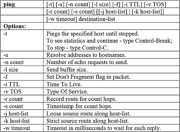
Procedure:
- Run Command Prompt; startup the Wireshark packet sniffer and start packet capturing
- Type “ping –n 5 hostname” in DOS Command line where, hostname is a host, the argument “–n 5” indicates that 5 ping messages should be sent. Then run Ping program by typing return.
- Stop the packet capture in Wireshark when the Ping program terminates.
- At the end of the experiment, your command prompt window should look like figure shown below.

Command Prompt window after Ping command
- Figure below resembles the screen shot of Wireshark output after filtering the ‘icmp’ messages. Note that the packet listing shows 10 packets: the 5 Ping queries sent by the source and the 5 Ping responses received by the source. Look into the first packet content area; the IP datagram within this packet has protocol number 01, which is the protocol number for ICMP packet.
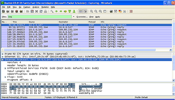
Wireshark output for Ping program
- ICMP echo request:
- Examine the protocol type and time to live fields in the IP packet that carries the first ICMP Echo Request. ICMP packet doesn’t have source and destination port numbers. Why?
- Study the ICMP message and what are the fields does ICMP packet have? Check the number of bytes for the checksum, sequence number and identifier fields.
- Identify the data bytes in request message and note the corresponding character sequence in third pane of Wireshark window.
- ICMP echo reply:
- Compare the message identifier and sequence number in the reply message with the equivalent numbers in the request message?
- Recognise the data bytes in the reply message and compare the data sequence with that in the request message.
- For echo request and echo reply messages:
- How do the identifier and sequence numbers alter with time?
- Does the data sequence in the request and reply messages change?
- Calculate the time that elapses between the sending and receiving of each echo. Compare the time delays with those provided by the PING command.
Exercise 4:
Analyse structure of fragmented IP datagrams with a protocol analyser
Requirement:
- Wireshark software
Procedure:
- Start up the Wireshark packet sniffer program. Click Capture → Start → Choosing the appropriate network card.
- Start the web browser and open an ‘http://’ link provided by the instructor. Link makes a connection to the desired web server.
- Now, stop Wireshark packet capture. Wireshark window should look similar to the window shown below.

Wireshark packet capture screen result
-
- Capture the screen shot of the result window. Find the packet numbers of the HTTP GET message (sent from your computer to the web server) and response message (sent to your computer by the web server). Take notes of their packet numbers.
- Select the packet that contains the HTTP GET message. Expand the details of the Internet Protocol datagram. Look into the packet details and packet content windows of the HTTP GET message
Note: The HTTP GET message is carried inside a TCP segment, which is in turn carried inside an IP datagram, which is carried inside an Ethernet frame.
-
- What is the version of the IP protocol?
- What is the IP address of a destination computer?
- What is the size (bytes) of the IP datagram header?
- What is the total size (bytes) of the IP datagram?
- Has this datagram been fragmented? Explain how you determined whether or not the datagram has been fragmented.
- What is the purpose of the identification field? What is the identification of this IP datagram?
- Select the IP datagram containing the HTTP response message
- Has this datagram been fragmented?
- What is the identification of this IP datagram?
- What are the key differences between this IP datagram and the one containing HTTP GET message?
PRACTICALS – DAY-2
Exercise 5.a:
Scanning ports on hosts with Advanced Port Scanner
The instructor will install a web server (Xitami) on one of the hosts. There is no need to install a custom home page as the default home page is sufficient for this exercise. Alternatively connect the Netgear 526T switch to the network (do not replace a hub; just connect one of the switch ports to a hub port). Unfortunately the switch does not have an FTP server built in.
- After installing a port scanner (Advanced port scanner). Go to start menu- All programs – Advanced Port Scanner.

Port Scanner window
- Run the port scanner (e.g. Advanced Port Scanner or NMap) by clicking on ‘Scan’ button and ‘drill down’ in the display to observe the open ports on all machines. Most ports (such as 139) are related to Windows operation. Try and detect the host with the web server, i.e. the one displaying port 80.
- The following type of result will be obtained with the Advanced Port Scanner (‘Pscan’).
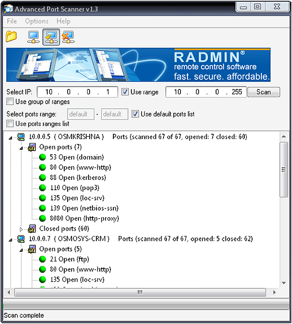
Port Scan Results
- Just to verify this, open the internet browser and type the IP address of the host with the web server. There is no need for the ‘http://’
If process described above does not work, then set up IE6 to look for web pages on the LAN and not, for example, on a dialup connection.
Exercise 5.b:
Scanning ports on hosts with NMap (Zenmap)
Port Scanning can also be performed using ‘NMap’ (Zenmap – provides graphical user interface)
- Install Nmap and complete the installation process following the wizard.
- Begin Zenmap by typing zenmap in a terminal or by clicking the Zenmap icon
 on the desktop.
 - To run the scan, type a target in the ‘Target’ field.
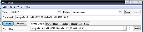
Zenmap main window showing a command and target
- The Command text box shows the output of the Nmap command while a scan is running or when it is completed.
- Target field can accept any number of targets, separated by spaces or comma. Zenmap supports all the commands or target specifications supported by Nmap. So, the targets such as 192.168.0.0/24, 10.0.0.* and 10.0.0-5.* will work.
Note: Select the host from the ‘Target’ dropdown box to re-scan a host.
- After specifying a target, run the Zenmap by clicking ‘Scan’ button.
- The following type of result (See Figure 6.4) will be obtained with the Zenmap port scanner.

Main Window
- Different aspects of the scan results are displayed in the five tabs (Nmap Output, Ports / Hosts, Topology, Host Details, and Scans) of the Zenmap window.
Each of these is shown below: - Nmap Output shows the familiar Nmap terminal output, displays all the open and closed ports of the hosts in the network.
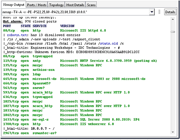
Results in Nmap Output
-
- Select a host in the left navigation pane (lists of hosts in the network). Ports/Hosts tab shows all the interesting ports on that host, along with version information when available.

Results in Ports/Hosts tab
-
- The “Topology” tab gives an interactive view of the connections between hosts in a network.

Results in topology tab
-
- The “Host Details” tab displays all the information about a selected host into a hierarchical display.
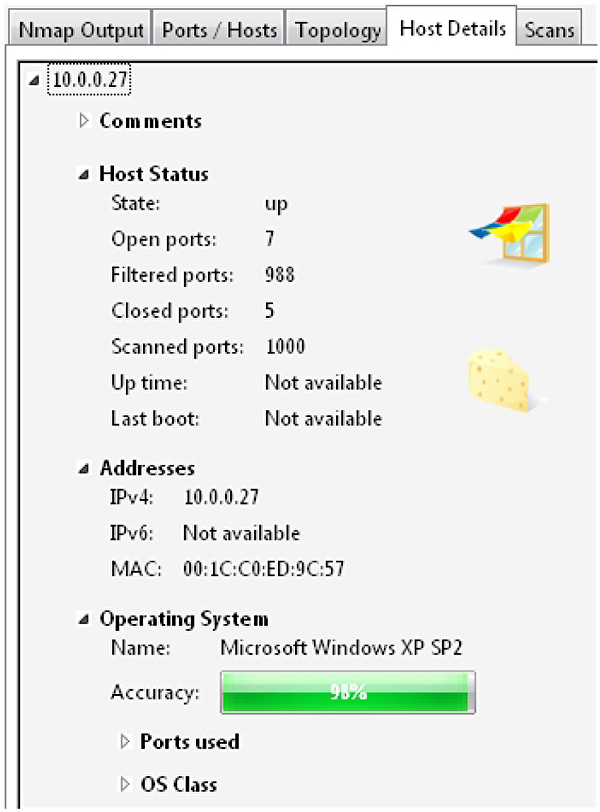
Results in Host Details tab
Exercise 6:
Checking TCP connections, sequence numbers and acknowledgments with Wireshark
Introduction
This exercise is to study TCP connection setup and investigate packet trace of the TCP file from client computer to a remote server using Wireshark. TCP Sequence Numbers and Acknowledgements are studied using Wireshark. Obtaining port numbers of the source and destination systems.
Requirement
- Wireshark software
Procedure
-
- Start the web browser and open an ‘http://’ link provided by the instructor.
- Link makes a connection to the desired web server.
- Now start Wireshark and begin packet capture (Capture->Options) and then click ‘Start’ on the ‘Wireshark Packet Capture Options’ screen (No need of selecting an option in this screen).

Wireshark main window
-
- Return to the browser and perform the operations directed by the instructor on the browser. Use either ‘POST’ or ‘Get’ method as per the instructor.
- Now, stop Wireshark packet capture. Wireshark window should look similar to the window shown below.

Wireshark window displaying TCP connection
-
- Enter ‘tcp’ (lower case only) into the filter text box located at the top of the Wireshark display window, and press return key after entering. This will filter the TCP packets displayed in the Wireshark window.
- Locate the initial three way handshake protocols containing – ‘SYN/SYN-ACK/ACK’.

Handshake protocols
-
- Confirm server and the client’s port numbers. The two port numbers involved are the ‘well-known’ port 80 (http) on the server side and the ‘registered’ port 4330 on the client side.
- The client port will vary but the 80 will not. The port numbers can be observed from the TCP header detail for the ‘SYN’ packet as seen in the Figure 6.4.

TCP Port details
-
- Check the actual Sequence and Acknowledgement numbers (x, x+1, y, y+1) used for the connection.
- The actual Sequence and Acknowledgement numbers (x, x+1, y, y+1) can be seen at the bottom of the screen by highlighting the appropriate Sequence and Acknowledge numbers in the middle of the screen. In Figure 6.5 the actual ISN (Initial Sequence Number) is ‘0x38cab8ff’, or ‘952 809 727’ in decimal.

Sequence number in hex
- Repeat the exercise, but this time the instructor will connect to the web server’s built-in FTP server by typing ‘ftp://’ in front of the IP address.
Note: This cannot be possible if the netgear switch used does not support FTP.
- Confirm that port 21 is used on the Server side.
- Scroll through the dialog followed by the TCP connection and try to get the password (in the form of an email address) used by the Client (anonymous login).
- Scroll through the FTP packets while observing the decoded data on the bottom right hand side of the screen, notice the user name (‘anonymous’) and the password resembling an email address in the format – ‘a@b.com’.
Exercise 7:
Replace hubs with switches and observe packet behaviour
A packet capture tool, Wireshark, can be used to monitor the packets going to and from a specific device. To be able to capture those packets, the packet capture tool has to be sharing the network segment.
One simple device that is useful to monitor another device’s packet flow is a hub. Using shared media or hubs to connect the Ethernet nodes together, meaning all packets could be received by all nodes on that network. Subsequently, all these packets can be monitored from any port on that hub. This shared feature makes Hubs a security risk.

Procedure:
-
- Set up a PC running Wireshark in it, to a network connected through hub as shown in figure above.
- Start Wireshark, and let it capture random packets for a minute or so. Now set up a host to ping another host on the same network.
- Monitor the captured packets as all packets on the network will be seen. Filter the captured packets so that we can limit the data between the two hosts.
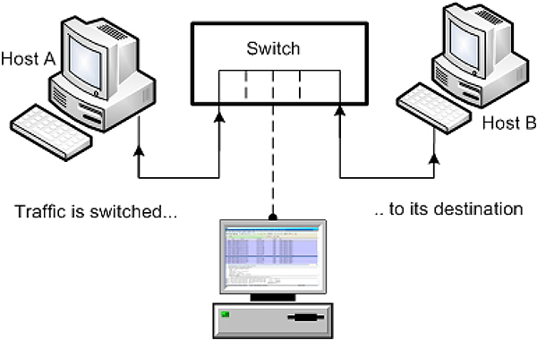
- Now replace hub with a switch or switch embedded into a router. Start running Wireshark. This will not allow a PC to monitor the packet flows of other devices.
Note: Switches optimize traffic and do not broadcast the data to all the computers in the network.
Exercise 8:
Convert laptop to simple 2-port router
If, for some reasons routers are not available, they may be replaced with two laptops set up as routers. The procedure for each laptop to act as a router is as follows:
- Insert two dissimilar network interface cards (NICs) into the laptop. It seems less problematic if the laptop’s built-in Ethernet interface is not used for this exercise.
- Set the IP addresses for the different NetIDs required, e.g. 192.168.0.1 and 200.200.200.2, or whatever is required. Refer to Figure 9.1
- Set the Default Gateway for each NIC as the ‘opposite’ IP address on the same machine, i.e. the default Gateway for 192.168.0.1 is 200.200.200.2, and vice versa.

IP setup for router
- Enable IP routing (IP forwarding). The method differs between various operating systems, but for XP and 2000 it is as follows:
- Click Start, Run and type regedit. Then follow the following path:
- Go to Hkey_Local_Machine \System \CurrentControlSet \Services\Tcpip \Parameters
- Change the value of IPEnableRouter to ‘1’, i.e. IPEnableRouter =Reg_Dword : 0x00000001 (1)
- Reboot and run ipconfig /all or wntipcfg to confirm that IP Routing is enabled.
The result is a simple two-port router. We are not running any dynamic routing protocols here, so we have to use static routing table entries (once again with reference to Figure 9.1).
For the ‘router’ on the left:
Route add 202.168.0.0 mask 255.255.255.0 200.200.200.1
For the ‘router’ on the right:
Route add 192.168.0.0. 255.255.255.0 200.200.200.1
These settings will disappear when the machine shuts down. To make them persistent across boots, you have to add the –p switch to the route commands shown above.
Exercise 9:
Tracing Ethernet packet contents between subnets with Wireshark
When troubleshooting a routed network at packet level, it is imperative to understand the actual (physical) movement of the packets, as opposed to the ‘logical’ sequence of events. In this exercise host ‘A’ (e.g. 192.168.0.2) will ping host ‘B’ (e.g. 202.168.0.2) repetitively (ping 202.168.0.2 –t), and capture the packets with Ethereal.
- Decide on a ping ‘sender’ and a ping ‘recipient. Then make a sketch on the whiteboard, and add the IP and MAC addresses of the following:
- Sender
- Router port on sender’s subnet
- Router port on recipient’s subnet
- Recipient
- Start pinging, and capture a few ICMP packets
- Look at the logical movement of the ICMP messages (‘from-to’), in terms of IP addresses, on the top section of the screen. It all looks ‘above board’.
Now select an ICMP Echo Message, go to the middle of the screen, and check the MAC addresses (source and destination) against your drawing. Suddenly things don’t look so right, or do they?
PRACTICALS – SOLUTIONS
Exercise 1:
IP configuration checks (ipconfig, wntipcfg)
- Check the configured IP address using ‘ipconfig’ command in Windows Command prompt.
- IPCONFIG (Internet Protocol Configuration) displays all the values of current TCP/IP network configuration and refreshes DHCP and DNS settings. It also has the additional versatility of interfacing with a DHCP server to renew a leased IP address.
- Command line options:

ipconfig options
-
- Click Start→run→cmd and then type ‘ipconfig /all’ from the DOS prompt. The result will look like the Figure 1.1. Note the MAC address of the host on which this command was executed: 00-A0-D1-4F-AD-59.

IP Configuration
The utility “wntipcfg” produces the same results. Click the ‘More Info’ tab and analyse details.

IP Configuration using wntipcfg utility
- No comments
- No comments
Exercise 2:
Connectivity checks (ping, arp, tracert)
-
- The following is a response to the ping command.

Ping messages
-
- The TTL shown is the value received back by the originator of the ICMP Echo Request message. Depending on the operating system on the target host, the ICMP Echo Reply message typically starts off with a TTL of 48 or 128. The fact that it is still the same when received by the originator indicates that there are no routers on the path to decrement it.
- The ‘arp’ table shows up as follows. The IP address/MAC entries shown are dynamic, i.e. they will expire in a few minutes unless refreshed.

MAC addresses
-
- This is a valid IP address, on the same subnet (although it does not exist) and therefore the ping will simply time out (no response).
- The target host is on a different subnet, but no Default Gateway is specified. The ping operation is therefore impossible and a ‘Destination Unreachable’ message is shown.
- No comment.
- The message is passed on to the Default Gateway. There is still no reply, but the first stage in the route is valid and therefore a timeout message is displayed (as opposed to ‘Destination Unreachable).
- The ARP table will show the router’s MAC address (since it is the next destination on the route). This can be confirmed by checking the router’s entry in the arp cache (ping it if necessary).
- Set up the ‘TJPingPro’ scan range in the top right hand corner of the ‘options’ window.

Figure 2.3
TJPingPro IP scan configuration- Now perform a sequential scan via the ‘seqscan’ button.

TJPingPro sequential scan results
-
- Whereas, ‘TJPing’ pings sequentially, ‘AngryIP’ (‘IPScan’) sets up a separate thread for each ping, i.e. it pings in ‘parallel’.

AngryIP scan results
-
- Use options→add columns, to add the Computer Name and MAC address columns.

AngryIP scan with additional columns
Exercise 9:
Tracing Ethernet packet contents between subnets with Wireshark
In this exercise host ‘A’ (e.g. 192.168.0.2) will ping host ‘B’ (e.g. 202.168.0.2) repetitively (ping 202.168.0.2 –t), and everybody will capture the packets with Ethereal.
- Make a copy of the following scenario (on the whiteboard, if you like), and add all IP addresses and MAC addresses of the following:
- Sender (ping originator)
- Router port on subnet 192.168.0.0
- Router port on subnet 202.168.0.0
- Ping recipient
- [(2) to (4)] your results will resemble as shown in the Figure 9.1. In terms of IP addresses everything looks fine, and the IP addresses given on the top display (line 14 in this case) correspond with those contained in the expanded IP header below.
When we look at the MAC addresses (Figure 9.2), things seem different. The sender’s MAC address is correct, but the recipient’s address seems wrong. It is, in fact, not the MAC address for 202.168.0.3, but that of the router (192.168.0.1) instead.

Details of Echo Request (IP header expanded)

Details of Echo Request (IP header expanded)
The explanation is simple. The packet travels from the sender to the first router, then from router to router, and ultimately to the ping recipient. Using protocol analyzers on the two subnets we can observe two parts of the journey: from sender to Router 2 and from Router 1 to recipient.
With suitable equipment it would also be possible to capture the packets traversing the cable between Router 1 and Router 2.

Professional Certificate of Competency in Advanced TCP/IP-Based Industrial Networking
Designed for engineers and technicians who need practical knowledge in…Read more
Professional Certificate of Competency in Allen Bradley Controllogix / Logix5000 PLC Platforms
Designed for engineers and technicians who need practical knowledge in…Read more
Professional Certificate of Competency in Arc Flash Protection
Designed for engineers and technicians who work in the electrical…Read more
Professional Certificate of Competency in Chemical Engineering and Plant Design
Designed for engineers and technicians who need practical knowledge in…Read more
Professional Certificate of Competency in Circuit Breakers, Switchgear and Power Transformers
Designed for engineers and technicians who need practical knowledge regarding…Read more
Professional Certificate of Competency in Control Valve Sizing, Selection and Maintenance
Designed for engineers and technicians who need a solid understanding…Read more
Professional Certificate of Competency in Electrical Power System Fundamentals for Non Electrical Engineers
Designed for engineers and technicians who need to understand the…Read more
Professional Certificate of Competency in Electrical Power System Protection
Designed for engineers and technicians who need practical skills and…Read more")
Professional Certificate of Competency in Electrical Wiring Standards: AS/NZS 3000:2018 (Australia and New Zealand Only)
This professional development course is designed for engineers and technicians…Read more
Professional Certificate of Competency in Fundamental E & I Engineering for Oil and Gas Facilities
Designed for engineers and technicians who need to update their…Read more
Professional Certificate of Competency in Gas Turbine Engineering
Designed for engineers and technicians who need practical skills in…Read more
Professional Certificate of Competency in Hazardous Areas and Intrinsic Safety For Engineers and Technicians
Designed for engineers and technicians who need to understand the…Read more")
Professional Certificate of Competency in Heating, Ventilation and Air-Conditioning (HVAC)
Designed for engineers and technicians from a wide range of…Read more
Professional Certificate of Competency in IEC 61850 Based Substation Automation
Designed for engineers and technicians who need to understand the…Read more
Professional Certificate of Competency in Industrial Data Communications
Designed for engineers and technicians who need to understand how…Read more
Professional Certificate of Competency in Instrumentation, Automation and Process Control
Designed for engineers and technicians who need to gain practical…Read more
Professional Certificate of Competency in Machine Learning and Artificial Intelligence
This professional development course is designed for engineers and technicians…Read more
Professional Certificate of Competency in Mechanical Engineering
This professional development course is designed for engineers and technicians…Read more
Professional Certificate of Competency in Onshore and Offshore Pipeline Systems
Designed for engineers and technicians who need to gain an…Read more
Professional Certificate of Competency in Power Distribution
designed for engineers and technicians who need to gain a…Read more
Professional Certificate of Competency in Practical Machine Learning Using Python for Engineers and Technicians
Designed to use Python Programming to work with machine learning…Read more
Professional Certificate of Competency in Practical Python for Engineers and Technicians
Designed for engineers and technicians who need to understand the…Read more & SCADA Systems")
Professional Certificate of Competency in Programmable Logic Controllers (PLCs) & SCADA Systems
Designed for engineers and technicians who need to get practical…Read more
Professional Certificate of Competency in Project Management for Engineers & Technicians
This professional development course is designed for engineers and technicians…Read more
Professional Certificate of Competency in Safety Instrumentation Systems for Process Industries
Professional development course designed for engineers and technicians who want…Read more
Professional Certificate of Competency in Sewage and Effluent Treatment Technologies
Designed for engineers and technicians who need practical skills and…Read more
Professional Certificate of Competency in Structural Design for Non Structural Engineers
Professional development course designed for engineers and technicians who need…Read more")
Professional Certificate of Competency in Substation Design (Main Equipment)
Professional development course is designed for engineers and technicians who…Read more")
Professional Certificate of Competency in Substation Design (Control, Protection and Facility Planning)
Designed for engineers and technicians who need to gain practical…Read more
Professional Certificate of Competency in the Fundamentals of Process Plant Layout & Piping Design
Professional development course is designed for engineers and technicians who…Read more
Professional Certificate of Competency in Practical Mechanical Sealing
This professional development course is designed for engineers and technicians…Read more
Professional Certificate of Competency in Road Construction
This professional development course is designed for engineers and technicians…Read more
Professional Certificate of Competency in Specification and Technical Writing
Master the art of writing clear, accurate, and professional technical…Read more
Professional Certificate of Competency in Hydraulics and Pneumatics
Overview of all aspects related to the construction, design, operation,…Read more
Professional Certificate of Competency in Big Data and Analytics in Electricity Grids
This course explores the use of big data & data…Read more
Professional Certificate of Competency in Renewable Energy Systems
This course covers various renewable energy systems that are popular…Read more
Professional Certificate of Competency in Smart Grids
A smart grid is an electricity network that uses digital…Read more
Professional Certificate of Competency in Hydrogen Energy – Production, Delivery, Storage and Use
Hydrogen energy short course designed for engineers and professionals interested…Read more")
Professional Certificate of Competency in Building Information Modelling (BIM)
This professional development course is covering practical aspects of using…Read more
Professional Certificate of Competency in Industrial Internet of Things
Internet of Things (IoT) is the most sort after technology…Read more