")
52896WA Advanced Diploma of Civil and Structural Engineering (Materials Testing)
Investigation of the properties of construction materials, the principles which…Read more")
Graduate Diploma of Engineering (Safety, Risk and Reliability)
The Graduate Diploma of Engineering (Safety, Risk and Reliability) program…Read more
Professional Certificate of Competency in Fundamentals of Electric Vehicles
Learn the fundamentals of building an electric vehicle, the components…Read more
Professional Certificate of Competency in 5G Technology and Services Overview
Learn 5G network applications and uses, network overview and new…Read more
Professional Certificate of Competency in Clean Fuel Technology - Ultra Low Sulphur Fuels
Learn the fundamentals of Clean Fuel Technology - Ultra Low…Read more
Professional Certificate of Competency in Battery Energy Storage and Applications
Through a scientific and practical approach, the Battery Energy Storage…Read more
52910WA Graduate Certificate in Hydrogen Engineering and Management
Hydrogen has become a significant player in energy production and…Read more
Professional Certificate of Competency in Hydrogen Powered Vehicles
This course is designed for engineers and professionals who are…Read more
This manual focuses on the critical project-related activities such as work breakdown, scheduling, cost control and risk management.
Revision 6
Website: www.idc-online.com
E-mail: idc@idc-online.com
IDC Technologies Pty Ltd
PO Box 1093, West Perth, Western Australia 6872
Offices in Australia, New Zealand, Singapore, United Kingdom, Ireland, Malaysia, Poland, United States of America, Canada, South Africa and India
Copyright © IDC Technologies 2012. All rights reserved.
First published 2002
ISBN: 978-1-921716-54-6
All rights to this publication, associated software and workshop are reserved. No part of this publication may be reproduced, stored in a retrieval system or transmitted in any form or by any means electronic, mechanical, photocopying, recording or otherwise without the prior written permission of the publisher. All enquiries should be made to the publisher at the address above.
Disclaimer
Whilst all reasonable care has been taken to ensure that the descriptions, opinions, programs, listings, software and diagrams are accurate and workable, IDC Technologies do not accept any legal responsibility or liability to any person, organization or other entity for any direct loss, consequential loss or damage, however caused, that may be suffered as a result of the use of this publication or the associated workshop and software.
In case of any uncertainty, we recommend that you contact IDC Technologies for clarification or assistance.
Trademarks
All logos and trademarks belong to, and are copyrighted to, their companies respectively.
Acknowledgements
IDC Technologies expresses its sincere thanks to all those engineers and technicians on our training workshops who freely made available their expertise in preparing this manual.
Contents
Chapter 1 – Fundamentals 1
1.1 Definitions 1
1.2 Project Management 2
1.3 Project Life Cycle 4
1.4 Project organizations 6
1.5 Project success 11
1.6 Project planning 13
Chapter 2 – Time Management 23
2.1 Project Planning 23
2.2 The critical path method 24
2.3 The precedence method 31
2.4 Presentation of the scheduled network 34
2.5 Analyzing resources requirements 35
2.6 Progress monitoring and control 37
2.7 Software selection 39
Chapter 3 – Cost Management 41
3.1 Cost estimating 41
3.2 Estimating methods 42
3.3 Forecast final cost 43
3.4 Documentation of estimating procedures 43
3.5 Budgeting 43
3.6 Financial control 44
3.7 Change control 45
3.8 Cost reporting 47
3.9 Value management 48
Chapter 4 – Risk Management 49
4.1 Definition of ‘risk’ 49
4.2 Risk management 50
4.3 Establishing the context 51
4.4 Risk identification 52
4.5 Risk analysis 53
4.6 Risk evaluation 58
4.7 Risk treatment 59
4.8 Monitoring and review 60
Chapter 5 – Quality Management 65
5.1 Quality and quality management basics 65
5.2 Quality assurance systems 71
5.3 ISO 9000:2005 Quality System guidelines 72
5.4 Project quality assurance 73
Chapter 6 – Integrated Time and Cost Management 77
6.1 Earned value analysis 77
6.2 EVM analysis illustrated 79
6.3 Computer based integrated time and cost control 81
Chapter 7 – The Project Manager 83
7.1 Management and leadership 83
7.2 Cultural influences on project management 86
7.3 Authority and power of the project manager 90
7.4 Required attributes of the project manager 91
7.5 Essential functions of project managers 91
7.6 Selection of the project manager 92
Chapter 8 – Contractual Issues in Procurement Contracts 95
8.1 The Commonwealth legal system 96
8.2 Elements of contracts 97
8.3 Procurement strategy issues 101
8.4 Tendering 104
8.5 Vitiating factors 105
8.6 Termination of contracts 106
8.7 Time for completion and extensions of time 108
8.8 Remedies for breach of contract 111
8.9 Liquidated damages for late completion 112
8.10 Penalties and bonuses 112
Chapter 9 – Exercises 115
9.1 Work breakdown structures 115
9.2 Time management 115
9.3 Cost management 116
9.4 Integrated time and cost 121
9.5 Quality management 123
9.6 Risk analysis 125
9.7 Contractual issues 126
9.8 Project quality plan 128
Chapter 10 – Solutions 129
10.1 Work breakdown structures 129
10.2 Time management 134
10.3 Cost management 143
10.4 Integrated time and cost 145
10.5 Quality management 147
10.6 Risk analysis 147
10.7 Contractual issues 151
10.8 Project quality plan 152
Appendix A – Budgets, Variance Analysis, Cost Reporting and Value Management 155
Appendix B – Cost Estimation Methods 211
Appendix C – Reference Cases 325
Learning objectives
The objective of this chapter is to:
- Provide an introduction to the concept of project management. This includes fundamental definitions, basic project management functions, project life cycles and phases
- Review the types and influences of alternative organization structures, with respect to both the organizations within which projects are undertaken, and the organization of the project team
- Review the issues fundamental to successful project outcomes
- Review the essential elements of effective project planning and control
This overview will show how the specific planning and control techniques introduced during the course are incorporated into the project management function.
These concepts are applicable to the management of projects of any type. While specific industries and certain types of projects will often require specialist knowledge to effectively plan and control the project, the principles outlined in this course will generally apply in all cases.
The definitions and techniques presented here are generally accepted within the project management discipline. That is; their application is widespread, and there is consensus about their value.
1.1 Definitions
1.1.1 Project
Performance of work by organizations may be said to involve either operations or projects, although there may be some overlap.
Operations and projects share a number of characteristics in that they are:
- Planned, executed, and controlled
- Constrained by resource limitations
- Performed by people
Projects are, however, different from operations (such as maintenance or repair work) in that they are temporary endeavours undertaken to create a. unique product or service. Table 1.1 shows the differences and similarities between operational and project activities.
| OPERATIONAL ACTIVITY | PROJECT ACTIVITY | |
|---|---|---|
| Planned | Yes | Yes |
| Executed | Yes | Yes |
| Controlled | Yes | Yes |
| Resources consumed | Yes | Yes |
| Organization | Permanent | Temporary |
| Output | Non-unique | Unique |
The primary objectives of a project are commonly defined by reference to function, time, and cost. In every case there is risk attached to the achievement of the specified project objectives.
1.1.2 Program
A program is a grouping of individual, but inter-dependent, projects that are managed in an integrated manner to achieve benefits that would not arise if each project were managed on its own.
1.1.3 Project management
Project management is the application of specific knowledge, skills, tools, and techniques to plan, organise, initiate, and control the implementation of the project, in order to achieve the desired outcome(s) safely.
Note that ‘Project Management’ is also used as a term to describe an organizational approach known as ‘Management by Projects’, in which elements of ongoing operations are treated as projects, and project management techniques are applied to these elements.
1.2 Project management
1.2.1 Elements
Successful project management requires that planning and control for each project is properly integrated.
Planning for the project will include the setting of functional objectives, cost budgets and schedules, and define all other delivery strategies. Successful planning requires the proper identification of the desired outputs and outcomes.
Control means putting in place effective and timely monitoring, which allows deviations from the plan to be identified at an early stage. As a result they can be accommodated without prejudicing project objectives, and corrective action can be initiated as required.
A project organization appropriate to the task must be set up, and the duties and responsibilities of the individuals and groups within the organization must be clearly defined and documented. The lack of clear definition of structure and responsibilities leads to problems with authority, communication, co-ordination and management.
The project management procedures put in place for the project must ensure that monitoring is focused on the key factors that the results obtained by monitoring are timely as well as accurate, and that effective control systems are established and properly applied by the project team. Project management involves five basic processes:
- Initiating: Undertaking the necessary actions to commence the project or project phase
- Planning: Identifying objectives and devising effective means to achieve them
- Executing: Co-ordinating the required resources to implement the plan
- Controlling: Monitoring of the project and taking corrective action where necessary
- Closing: Formalising the acceptance of the project or phase deliverables (the ‘handover’), and terminating the project in a controlled manner
Within each of these processes there are a number of sub-process involved, all linked via their inputs and outputs. Each sub-process involves the application of skills and techniques to convert inputs to outputs. An example of this is the preparation of a project network diagram (output) by the application of the precedence method (technique) to the identified project activities (input).
1.2.2 The professional body of knowledge
Project management has developed as a professional discipline since the 1950s. It is claimed, reasonably, that the military was the first institution that adopted planning and control processes that could be characterized as formal project management – specifically for the Normandy invasion, and subsequently for the Manhattan Project. Since the 1970s there has been a sustained development of project management as a professional discipline.
There are professional project management bodies in most countries. In Australia the professional organization is the Australian Institute for Project Management. In New Zealand it is the New Zealand Chapter of the Project Management Institute (PMI). The international body is the International Project Management Association.
In defining the knowledge base for project management it is useful to refer to the structures adopted by the PMI in the USA and the Association for Project Management (APM) in the UK. Their web addresses are www.pmi.org and www.apm.org.uk respectively.
PROJECT INTEGRATION MANAGEMENT
PROJECT SCOPE MANAGEMENT
PROJECT TIME MANAGEMENT
PROJECT COST MANAGEMENT
PROJECT QUALITY MANAGEMENT
PROJECT HUMAN RESOURCE MANAGEMENT
PROJECT COMMUNICATIONS MANAGEMENT
PROJECT RISK MANAGEMENT
PROJECT PROCUREMENT MANAGEMENT
|
PROJECT MANAGEMENT
ORGANISATION and PEOPLE
TECHNIQUES and PROCEDURES
GENERAL MANAGEMENT
|
| IIA PMI PMBOK | IIB APM PMBOK |
1.3 Project life cycle
1.3.1 Lifecycle elements
Projects proceed through a sequence of phases from concept to completion. Collectively, the separate phases comprise the project ‘life cycle’.
There are only a limited number of generic lifecycles, though the breakdown of the phases within can be at differing levels of detail. The generic types are usually considered to include capital works, pharmaceutical, petrochemical, defence procurement, research and development, and software development. Consequently the initial starting point for managing the project is to define the type, and select an appropriate life cycle model as the planning framework.
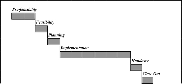
Figures 1.1 and 1.2 illustrate generic project life cycles for two project types.
Project life cycle: capital works project

Project life cycle: defence acquisition project
1.3.2 Project phases
Different industries generally have specific standard definitions for each phase, but a generic description of each phase identified in Figure 1.1 for a capital works project is:
- Pre-feasibility: Identification of needs, and preliminary validation of concept options
- Feasibility: Detailed investigation of feasibility, including preliminary brief, project estimate and investment analysis
- Planning: Detailed definition of the project with respect to scope, organization, budget, and schedule, together with definition of all control procedures
- Implementation: The execution of the scoped project. The components of this phase will depend upon the nature of the project
- Handover: Passing the facility into the control of the principal. This includes formal handover of the facilities, user training, operating and maintenance documentation etc.
- Close out: Archiving of the project records, establishing appropriate performance evaluations, capturing and transferring lessons learned, and dissolving the project organization
Project phases share defined characteristics.
- In every instance project management processes undertaken with a specific phase comprise initiating, planning, executing, controlling, and closing.
- A project phase will have one or more tangible deliverables. Typical deliverables include work products such as feasibility studies, software functional specifications, product designs, completed structures, etc.
- Outputs from a phase are typically the inputs to the succeeding phase
Normally, deliverables from any phase require formal approval before the succeeding phase commences. This can be imposed through the scheduling of compulsory ‘milestones’ (e.g. design reviews) between phases.
1.4 Project organizations
1.4.1 General
Where projects are set up within existing organizations, the structure and culture of the parent organization has great influence on the project, and will be a deciding factor in whether or not there is a successful outcome. Where the project team is outside the sponsoring or client organization, that organization may exert significant influence on the project.
The organization of the project team also directly influences the probability of achieving a successful outcome. The benefits and disadvantages of the various options for project team organization need to be appreciated.
1.4.2 Projects within existing organizations
Organisational structures have traditionally been defined within the spectrum from fully functional to fully project oriented. Between those extremes lie a range of matrix structures.
The classic functional structure is a hierarchy, with staff grouped within specialist functions (e.g. mechanical engineering, accounting etc.), with each staff member reporting directly to one superior. Such organizations do manage projects that extend beyond the boundaries of a division, but within a division the scope of the project is considered only as it exists within the boundary of that division. Project issues and conflicts are resolved by the functional heads.
In a project management organization the staff are grouped by project, and each group headed by a project manager who operates with a high level of authority and independence. Where departments co-exist with the project groups, these generally provide support services to the project groups.
Matrix organizations may lie anywhere between the above. A matrix approach applies a project overlay to a functional structure. Characteristics of matrix organizations may be summarised as follows:
- Weak matrix organizations are those closely aligned to a functional organization, but with projects set up across the functional boundaries under the auspices of a project co-ordinator. The project co-ordinator does not have the authority that would be vested in a project manager
- A strong matrix organization would typically have a formal project group as one of the divisions. Project managers from within this group (often with the necessary support staff) manage projects where specialist input is provided from the various functional groups. The project managers have considerable authority, and the functional managers are more concerned with the technical standards achieved within their division than with the overall project execution
- In a balanced matrix the project management is exercised by personnel within functional divisions who have been given the appropriate authority necessary to manage specific projects effectively
The different organizational structures, and the corresponding project organization options, are identified in Figure 1.3. In many cases an organization may involve a mix of these structures at different levels within the hierarchy. For example, a functional organization will commonly set up a specific project team with a properly authorized project manager to handle a critical project.
The influence of the organization structure on various project parameters is illustrated in Figure 1.3.
While a matrix approach may be seen as providing an inadequate compromise, in reality it is often the only realistic option to improve the performance of a functional organization. It does work, but there are some trade-offs. One factor critical to the effectiveness of the matrix structure is the authority vested in the person responsible for delivery of the project. A key predictor of project performance is the title of this person i.e. whether he/she is identified as a ‘project manager’, or something else.
Briefly, the benefits and disadvantages of the matrix approach include (see Table 1.3), also see Table 1.4:
| Benefits | Disadvantages |
|---|---|
| All projects can access a strong technical base | Dual reporting structures causes conflict |
| Good focus on project objectives | Competition between projects for resources |
| Sharing of key people is efficient | There may be duplication of effort |
| Rapid responses to changes | Management and project goals in conflict |
| Individuals have a protected career path |

Project structures within organizations
| Organization type | Functional | Weak matrix | Balanced matrix | Strong matrix | Project |
|---|---|---|---|---|---|
| Project mgr Authority | Little or none | Limited | Low to moderate | Moderate to high | High to Total |
| % Personnel assigned 100% on project | Minimal | 0-25% | 15-60% | 50-95% | 85-100% |
| Project mgr Role | Part time | Part time | Full time | Full time | Full time |
| Project mgr Title | Co-ordinator/Leader | Co-ordinator/Leader | Project manager | Project manager | Project manager |
| Project mgr Support staff | Part time | Part time | Part time | Part time | Full time |
1.4.3 Project organization
The organization of the project team is characterised by:
- The principal or project sponsor. This is the beneficial owner of the project
- The Project Control Group (PCG). In some cases this will be the principal, but when the principal is a large company it is required to identify and make accountable certain nominated individuals. The function of this group is to exercise approvals required by the project manager from time to time, controlling the funding to the project manager, and maintaining an overview of the project through the reporting process
- The project manager. In a ‘perfect world’ the responsibilities, roles and authority of this person would be defined and documented
- A project control officer or group, if this function is not undertaken by the project manager. This group of people is responsible for the acquisition and analysis of data relating to time, cost and quality, and to compare actual figures with the planned figures
- The rest of the project team, which will vary in composition according to the project type, as well as specific project variables
The project organization may be vertical or horizontal in nature, depending on the span of control chosen by the project manager. That choice will be a balance between available time and the desired level of involvement. Typical project structures for a capital works project are illustrated in Figure 1.4. These illustrate the difference between horizontal, intermediate, and vertical organization structures.
In general the horizontal structure is the best option, because the communication channels between those who execute the project work and the project manager are not subject to distortion. For instance, in the vertical organization there is a far higher probability of the project manager receiving and acting upon inaccurate information. Such inaccuracies may arise unavoidably, by oversight, carelessly, or deliberately. The impacts can be severe. Reducing that opportunity, by shortening communication channels and removing the intermediate filters, improves the likelihood of achieving the desired project outcome.
On large projects the desire to maintain a horizontal structure can be largely achieved by increasing the size of the ‘project manager’. This is typically done by augmenting the project manager with support staff that have direct management responsibilities for a portion of the project. Their interests are aligned with those of the project managers, and a higher reliability of information may be expected.

Project team organization
1.5 Project success
1.5.1 General
Many projects qualify as successes, but we all have experience, anecdotal or otherwise, of projects that have gone severely wrong. Project failures exist within all industries. Even today, with the level of awareness for project management processes as well as advanced tools, there are spectacular failures. These occur even on very large projects where it is assumed that the investment in management is high. The consequences of failure can be significant to the sponsoring organizations as well as project personnel.
A 1992 study of some 90 data processing projects, completed in the previous 12 years, provides a common profile of experience. The study identified the primary factors affecting the project outcomes as set out in the Table 1.5. These are listed by frequency and severity (ranked in descending order of impact) in respect of their negative impact on project success. This analysis provides an instructive basis for any organization operating, or setting up, a project management methodology. Note that most of these issues are project management issues.
| Factor | Frequency | Severity |
|---|---|---|
| Planning/monitoring | 71% | 1 |
| Staffing | 58% | 2 |
| Scope management | 48% | 3 |
| Quality management | 44% | 4 |
| Communications | 42% | 5 |
| Technical | 36% | 7 |
| Management | 32% | 8 |
| User involvement | 30% | 6 |
| Implementation issues | 28% | 9 |
| Operations | 24% | 11 |
| Organization | 24% | 10 |
| Estimating | 19% | >12 |
1.5.2 Project success criteria
It is a vital step, yet one commonly omitted, to define the project success criteria before commencing planning and delivery. In other words, define what needs to be achieved if the project implementation is to be considered a success. The project stakeholders must identify and rank the project success criteria. The ‘client’s’ preferences are obviously paramount in this process, and will consider performance right through the life of the product under development as well as the factors present only during the project.
The objectives of cost, quality, and time are frequently identified as the definitive parameters of successful projects. These are a very useful measure in many capital works projects where they can be defined in advance, adopted as performance indicators during project implementation, provide a basis for evaluating trade-off decisions, and applied with relative simplicity.
However, this approach to measuring project success is necessarily only a partial assessment in almost every situation. Projects completed within the targets for such constraints may be successfully completed from the perspective of the project implementation team, but are not necessarily from alternative viewpoints such as those of the sponsors or users. In some instances projects that are not completed within some of the time/cost objectives may still be considered a success. Common project success criteria include safety, loss of service, reputation, and relationships.
The process of defining ranked success criteria provides surprising insights in many instances, and enhances project planning. During project implementation the project success criteria provide a meaningful basis for establishing project performance indicators to be incorporated within project progress reports. They are also helpful in making trade-offs, should that become necessary.
1.5.3 Critical success factors
The results of a study of the critical success factors in projects, published in the June 1996 issue of the International Journal of Project Management, proposes a framework for determining critical success factors in projects. This study classified critical success factors applicable to all project types within four interrelated groups. These are set out in Table 1.6 with examples.
| Factors related to: | Example |
|---|---|
| The specific project | Project size, complexity, technology, number of interfaces |
| The project manager and team | Project management expertise, authority, systems, personality, resources |
| The customer organization | Customer commitment, response times, knowledge |
| The external environment | Environment: social, cultural, political, economic, financial, technical |
In practice, this is a particularly important and useful framework within which critical success factors can be identified. Where necessary, these can be managed proactively in order to maximise the probability of project success.
A survey was conducted amongst members of the PM, seeking to correlate project success criteria (specified as time, cost, quality, client satisfaction, and other) against the above factors. Projects included in the survey covered construction, information services, utilities, environmental and manufacturing. The study concluded that the critical project success factors primarily arose from the factors related to the project management and project team. For each industry the project manager’s performance and the technical skills of the project team were found to be critical to project outcomes. This confirms the conclusions from the 1992 study noted earlier.
It is important to identify, within this framework, the specific critical success factors which may impact on the project. It is then the reponsibility of the project team to develop strategies to address these factors, either in the planning or in the implementation phase.
1.5.4 Critical project management issues
The skills, knowledge, and personal attributes of the selected project manager have a critical impact on the success of the project. These critical skills encompass more than just technical and project management parameters. A key element in the success of the project manager is the effective application of non-technical skills (the so-called ‘soft’ skills); including leadership, team building, motivation, communication, conflict management, personnel development and negotiation.
It is essential that the project manager, once appointed, has full control of the project within the limitations defined by the principal or project sponsor. All parties must be made aware of this single point of authority. The authority delegated to the project manager, and his/her effectiveness in exercising it, is critical. Project management structures, particularly if the project is one within an existing organization and across functional boundaries, creates a complex web of formal and informal interactions. Lack of clarity in defining the authority of the project manager invariably leads to difficulties.
The appointment of the project manager should ideally be made sufficiently early in the project to include management of the feasibility studies. The project manager should be appointed in order to undertake the project definition. If the project manager is not involved in the project definition phase, the outputs of this phase (project plan, control procedures, etc.) must be specifically signed off by the project manager when subsequently appointed to that role.
1.6 Project planning
1.6.1 The project quality plan
“PROJECTS BADLY PLANNED ARE PROJECTS PLANNED TO FAIL”
The project planning phase is critical to the effective implementation and control of the project and the basis for project success is established during this phase. The planning undertaken at this stage is the responsibility of the project manager. The primary output from this phase is the Project Quality Plan (PQP). The basic element required to properly define the PQP is the Work Breakdown Structure or WBS.
The PQP comprises the following:
- The PQP sign-off
- The statement of project objectives
- The project charter
- The project plan
- Project control procedures
Note: here lies an inconvenience of terminology. The PQP is much more than a plan for incorporating quality into the project. There is a comnponent within the PQP that deals exclusively with quality issues per se.
1.6.2 PQP sign off, project objectives, project charter
PQP sign-off
This is a formal record of the agreement, signed by the Project Manager as well as the PCG of the PQP. It is confirmation of approval of the plan (e.g. what is to be done, when, who, at what cost etc) and the processes involved if the desired outcomes are to be achieved.
Project objectives
This is a statement defining the project objectives. The confirmed Project Success Criteria should be included, together with quantified measures. Unquantified objectives introduce a high degree of risk to the process, by reducing the ability to measure divergences at an early stage.
Project charter
Management’s commitment to internal projects (and hence the willingness to make available the required resources), as well as formal delegation of authorities to the project manager, are recorded here.
1.6.3 The project plan
The Project Plan is the master plan for the execution of the project, and provides the framework from which the implementation will develop in a co-ordinated and controlled manner. The project scope definition, programme and budget are established at this time. These provide the baseline against which performance can be measured, and against which approved changes to the project baseline can be properly evaluated. The Project Plan comprises the following components:
Scope definition
A written scope statement that defines, in appropriate detail, the scope of every project component and identifies all significant project deliverables. In this context ‘scope’ includes features and functions of products and/or services, and work to be undertaken to deliver a conforming output
Work breakdown structure
A Work Breakdown Structure (WBS) is the breakdown of the project into the separate activities that can be considered entities for the purpose of task assignment and responsibilities. The WBS is generally presented in a product-oriented hierarchical breakdown. Successive levels include increasingly detailed descriptions of the project elements. The lowest level items are referred to as work packages and these are assignable to individuals within the project team, or to subcontractors.
Orgonization breakdown structure
The Organization Breakdown Structure (OBS) involves the definition of the project structure, setting out the parties and individuals involved in the execution of the project. It also formalizes the lines of communication and control that will be followed.
Task assignment
This is a list of the assignment tasks and responsibilities. All tasks and activities previously defined become the responsibility of specified parties. The WBS and OBS may be extended to define a ‘task assignment matrix’.
Project schedule
The preliminary master schedule for the project identifies the target milestones for the project, and the relative phasing of the components.
Project budget
In some cases a project budget is established during the feasibility study, without the benefit of adequate detail of the concepts evaluated. At that stage a maximum cost may have been established, because expenditure above that figure would cause the project not to be economically viable. Where such a constraint exists, and if the feasibility study has not reliably established the cost of the project, it will be necessary to further develop the design before committing to the project.
Miscellaneous plans
Additional plans may need to be documented here. These include, inter alia, consultations and risk management. Alternatively, a strategy for these can be defined in the section dealing with project controls.
Documentation
All of the above project elements must be documented in the Project Plan. Figure 1.5 shows the inter-relationships of all these entities.

The project plan
1.6.4 Project control procedures
The ultimate success of the project will require that objectives for performance, budget and time, as defined within the Project Plan, are fulfilled. This will only be possible if the necessary monitoring and control systems are established prior to the commencement of project implementation.
Monitoring and reporting should include project performance indicators derived from the Project Success Criteria. Planning should take into account the critical success factors, i.e. it should address any potential difficulties that may arise from them.
Control procedures need to be established and documented for the management of the following parameters:
Administration
Procedures for the administration of the project should be defined. These should include issues such as:
- Filing
- Document management
- Correspondence controls
- Administrative requirements of the principal
Scope
The definition of scope change control systems which:
- Define circumstances under which scope changes can arise
- Control the process invoked when changes do arise
- Provide for integrated management of the consequences of the changes, i.e. time and cost implications
Quality
The definition of project-specific quality policies and standards, together with processes for ensuring that the required quality standards will be achieved. This is best achieved by reference to the application of, and responsibilities for, Inspection and Test Plans.
Cost
The definition of control procedures which should include:
- Budget and commitment approvals for design, procurement and construction functions
- The issue and control of delegated financial authority, to the project manager controlling consultants and contractors, as well as to consultants controlling contractors
- Variation control for changes arising during project implementation
- Value engineering
- Cost monitoring, reporting and control systems and procedures
Time
The definition of strategies and procedures for scheduling, monitoring and reporting, likely to include:
- Programming methods and strategies for master and detail programmes, i.e. definition of programming techniques as well as the frequency of review and updating
- Progress monitoring and reporting systems and procedures.
Risk
The definition of objectives and procedures for putting in place effective risk management. Note that there may be a Risk Management activity schedule in the PQP.
Communications
This specifies all requirements for communications within the project and to the client/sponsor, and is likely to include:
- Meetings – schedules and processes
- Reporting requirements
- Document distribution
- Handover
- Close out
Procurement
This defines strategies and procedures for tendering, as well as for the selection and management of consultants, suppliers and contractors.
Tendering
This covers documented standardized tendering procedures, tender documentation, and tender evaluation procedures for each contract type (i.e. service, procurement, construction etc).
The tendering process is often a very sensitive one, especially if public funds are involved. Appropriate attention must be paid to ensure that the legal aspects of the process are properly addressed, and that the process is applied with demonstrable fairness. Recent changes in the laws applying to tendering should be noted.
Consultants
This refers to a standardized document dealing with the use of consultants. It should cover issues such as consultants’ briefs and terms of engagement. Consultants’ briefs would typically include the following items:
- The scope of the work to be undertaken, and any limitations thereon
- The type of services to be provided and the deliverables required (this will be defined within the WBS for the specific work package)
- Approvals required from the client
- Approvals to be exercised on behalf of the client
- Special requirements of a management, technical or financial nature, for example quality assurance/quality control programmes, variation control procedures etc.
- Reporting requirements
- Project schedule requirements, for service delivery as well as implementation phases
- Budgets for the proposed implementation deliverables or capital items
- Basis of payment for services to be provided by the consultant
Contracts
The terms of engagement and conditions of contract should be based on standard documents where these exist. The level of documentation should be appropriate to the values of contracts let, and usually a number of options are required.
1.6.5 Work breakdown structures
Developing the WBS is fundamental to effective planning and control for the simple reason that the derived work packages are the primary logical blocks for developing the project time lines, cost plans and allocation of responsibilities.
Many people either miss out this key step in the project management process, or undertake the step informally without appreciating how important it is.
Definition and terminology
PMI PMBOK 1996 provides the following definition for a WBS:
A deliverable oriented grouping of project elements which organizes and defines the total scope of the project: work not in the WBS is outside the scope of the project. Each descending level represents an increasingly detailed description of the project elements.
The WBS is created by decomposition of the project, i.e. dividing the project into logical components, and subdividing those until the level of detail necessary to support the subsequent management processes (planning and controlling) is achieved.
Terminology varies in respect of defining project elements. The use of the terms ‘project’, ‘phase’, ‘stage’, ‘work package’, ‘activity’, ‘element’, ‘task’, ‘sub-task’, ‘cost account’, and ‘deliverable’ is common:
PMBOK terminology provides the following definitions:
- A work package is a deliverable at the lowest level of the WBS
- A work package can be divided into activities
- An activity is an element of work performed; with associated resource requirements, durations and costs
- An activity can be subdivided into tasks
A properly developed WBS provides a basis for:
- Defining and communicating the project scope
- Identifying all components of work within the project
- Identifying the necessary skills and resources required to undertake the project
- Effective planning of the project (scheduling, resource planning, cost estimating)
The WBS does not identify dependencies between the components, nor does it identify timing for the components. These are, for example shown in the PERT and Gantt charts (see next chapter).
Creating the WBS
There are many valid approaches for the decomposition of a project. In many cases there will be semi-standard WBS templates that can be used or adapted. The WBS should generally identify both the project management and project deliverables, and should always be defined to reflect the particular way in which the project is to be managed.
The appropriate level of detail will vary between projects, and at different times within the same project. Future project phases may need less definition than the current phases – so the WBS may be progressively developed as the project develops – but this requires a flexible WBS structure to be selected in the first instance.
In planning the WBS, criteria can be adopted to ensure that the level of detail is appropriate and consistent. Such criteria might include:
- Are the packages of work in the WBS sensible?
- Can any package be broken down further into sensible components?
- Is each package the responsibility of only one organizational group?
- Does every package represent a reasonable quantity of work?
- Does any package constitute more than, say, 5% (or 10%) of the project?
- Does any package constitute less than, say, 1% (or 2.5%) of the project?
- Does every package provide the basis for effective cost estimating and scheduling?
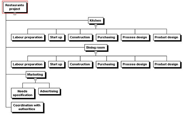
The following example shows the WBS of a project with geographical location at the second level (see Figure 1.6).

WBS for restaurants project
Alternatively, the various functions (design, build, etc) can be placed at the second level (see Figure 1.7).

Alternative WBS for restaurants project
A third alternative shows a subsystem orientation (see Figure 1.8).
Alternative WBS for restaurants project
A fourth alternative shows a logistics orientation as follows (see Figure 1.9):

Alternative WBS for restaurants project
The WBS could also be drawn to show a timing orientation (see Figure 1.10).

Alternative WBS for restaurants project
Note that ‘Design’ and ‘Execution’ in the WBS above are NOT work packages, they are just headings. ‘Start up’, however, is a work package since it is at the lowest level in its branch. The WBS could be broken down even further but the risk here is that the lowest-level packages could be too small. If ‘advertising’, for example, could be accomplished in 100 hours it might be a good idea to stop at that level. It could then be broken up into activities and tasks (and even sub-tasks); the duration and resource requirements would then be aggregated at the ‘advertising’ level, but not individually shown on the WBS.
It is, of course, not necessary to use a sophisticated WBS package; a spreadsheet will work just fine as the following example shows (see Figure 1.11).
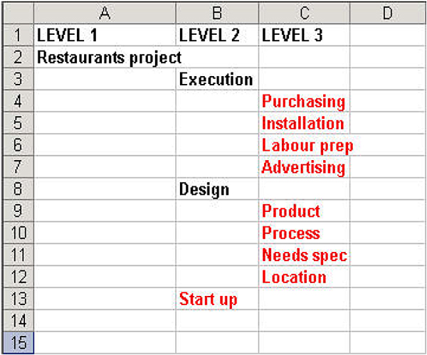
WBS using spreadsheet
Learning objective
The objective of this chapter is to provide a comprehensive introduction to the key elements of effective time management for projects. Time management of a project consists of:
- Planning the project activities to a time scale (i.e. the project schedule)
- Monitoring performance of the implementation phase
- Comparing achieved performance with the project schedule
- Taking corrective action to ensure planned objectives are most likely to be met
The level of project planning that we propose requires a significant input of time and energy at the start of the project, but considerably reduces the content and cost of management effort during the project implementation phase. The preparation of the project schedule is only the first, albeit very important, step.
Time management requires the monitoring and control functions to be carried out effectively so that the project schedule can be adhered to, or so that any variance from the plan does not prejudice project objectives.
The planning, monitoring and controlling cycle should be in process continuously until the project is completed. The project schedule should be prepared with some knowledge of the monitoring system to be employed. The prerequisite for setting up the monitoring system is the identification of the key factors to be controlled. It may be, for example, the achievement of specific milestones or particular resource items. The project manager will have to establish the boundaries within which these factors need to be constrained. Performance monitoring must focus on outputs, not inputs; i.e. results not effort.
2.1 Project planning
The principal aim of project management is to effectively utilize the available resources in order to achieve the planned objective(s).
It is most unlikely, if not impossible, that this aim can be achieved in the absence of rational planning and scheduling of all component activities, together with the associated human, material and financial resources. Particular techniques have been developed which allow this essential planning to be undertaken.
The most commonly used in the field of project management are known collectively as Project Network Techniques. These comprise:
- The ‘Critical Path’ method (also known as the Activity on Arrow or AoA method)
- The Precedence method (also known as the Activity on Node or AoN method)
The Critical Path method may be the only one many people are familiar with since it is intuitively attractive. The Precedence method appears, at least from a superficial look at the comparable diagrams, to be more complex.
However, the Precedence method is far more flexible. The Precedence method has the advantage of requiring no dummy activities to establish the correct logic for a project. Once the superficial complexity is overcome, you will find it to be the more powerful tool. Most computer-based project scheduling software packages use precedence logic and a proper understanding of the method enables the software to be used to best effect.
Precedence network analyses are normally presented graphically, either as the network diagram itself, or as a time-scaled bar chart known as a Gantt chart. Critical path networks can be presented as time-scaled arrow diagrams, or as Gantt charts. All computer-based project scheduling software packages use Gantt presentations in addition to the network diagrams.
Project analysis by either method involves the same four steps:
- Defining the activities. For the initial project plan this may involve the breakdown of work packages used as the basic elements for the other components of the PQP
- Preparation of the logic sequence to determine the relationships between the activities
- Applying activity (time and resource) data for each activity
- Analysis of the network
The following is a brief introduction to these techniques. It will, however, be sufficient to allow you to fully apply both methods to analyze any situation. There is a vast amount of literature available on the subject that could be consulted for additional guidance.
2.2 The critical path method
2.2.1 Defining the activities
The first step in project planning is to break the defined work packages into component activities, and sometimes tasks. It is crucial that this breakdown be carefully considered if the subsequent output is to be an effective project control tool.
In establishing the activity list, the following principles may assist:
- For an initial analysis the number of activities should be kept to the minimum required to be useful. This allows for the framework to be developed and checked for consistency before too much effort has been spent. If found necessary, the activities can be broken down further at a later stage if that is appropriate
- For a definitive plan it is useful to include more detail so that the schedule in the PQP can be adopted as the baseline for schedule monitoring
- Who else will be using the schedule, and for what purpose?
- Is it an appropriate master plan, allowing elements to be defined in more detail as implementation continues?
It is important to note that the word ‘operation’ or ‘activity’ is used in its widest sense. It will not only include actual physical events, derived form the work packages, but anything that may exercise a restraint on the completion of the project should be included as an activity. This will include actions such as obtain finance, obtain approval, place order, and represent passages of time with no actual activity, e.g. delivery period.
2.2.2 Preparing the logic network
The arrow diagram
In CPM, each activity is represented by an arrow. The tail of an arrow marks the start of the activity it represents, and the head marks its finish. The start and finish of activities are called events or nodes. Circles are drawn at the tails and heads of arrows to denote the nodes. The arrow diagram, or network, is drawn by joining the nodes together to show the logically correct sequence of activities. The arrows are not drawn to scale; their lengths are unimportant at this stage. Their directions show the flow of work. Here are a few simple illustrations.
Figure 2.1 shows two sequential activities indicating that Activity B cannot be started until Activity A is completed.

Network example
Figure 2.2 shows that Activity E must await the completion of both Activities C and D before it can commence.

Network example
Figure 2.3 shows Activities G and H as concurrent activities that can start simultaneously once Activity F has been completed.

Network example
When developing the arrow diagram, three questions are asked of each activity in order to ensure its logical sequence:
- What must precede it?
- What has to follow it?
- What can take place concurrently with it?
The importance of these three questions cannot be overemphasized. Be aware of the ease of inadvertently introducing constraints by implication.
Numbering of events
All events are numbered to facilitate identification. This step is usually carried out after the whole arrow diagram has been drawn. Each activity is identified by two event numbers, e.g. as (i,j). The (i) number identifies the tail of the arrow, and the (j) number identifies the head of the arrow. The letters ‘i’ and ‘j’ are chosen at random and have no special significance, but it is advisable to use multiples of 5 or 10. The reason for this is the flexibility to introduce additional events into the network. For example, see Figure 2.4.
Activity C is identified by (15, 20), D by (20, 25) and E by (20, 30). Note that for sequential activities, such as C and D, the (j) number of the preceding activity is the same as the (i) number of the following activity.

Numbering of activities
Dummies
Each activity should have a unique identification. If two concurrent activities both start and finish at the same nodes they will be identified by the same (i, j) numbers, as shown in Figure 2.5 where both Activities M and N are (15, 30).
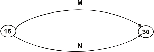
Concurrent activities
In order to keep the identification of activities unique, a dummy activity is introduced as shown in Figure 2.6. Activity M is still (15, 30) but Activity N is now (15, 25). Activity (25, 30) is a dummy. Dummy activities are always represented by a dotted arrow.

Dummy activities
Another important use for dummies is to keep the sequence logic correct in a group of arrows where not all preceding and following activities are interdependent. Suppose we have a situation where starting Activity D depends on the completion of both Activities A and B, and starting Activity C depends only on completion of Activity A.
The logic shown in Figure 2.7 is incorrect. It introduces a non-existent restraint, namely that Activity C cannot start until Activity B is complete.

Incorrect logic
The correct logic requires the introduction of a dummy activity. Refer to Figure 2.8.
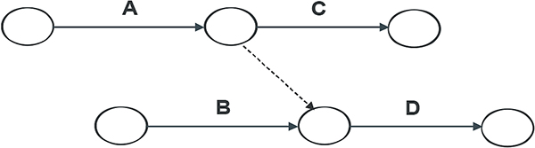
Correct logic
Overlapping activities
Unlike the conventional bar chart, no overlapping of activities is permitted in the arrow diagram. If overlapping exists between activities, then these activities must be broken down further to provide sequential activities that may subsequently be analyzed.
Figure 2.9 shows two sequential activities, indicating that Activity 2 starts after all of Activity 1 is complete.

Non-overlapping activities
For a small job, this is probably the case. For a large job, however, the two activities may overlap to some extent. This is shown by breaking both activities down into two activities, as shown in Figure 2.10.

Overlapping activities
2.2.3 Adding activity data
The way in which the necessary data is included on the network diagram is very simple. See Figure 2.11. The required information is added for each activity in the network. Once all necessary activities are included, the network can be analyzed.
Activity data
2.2.4 Analyzing the network
This analysis comprises the following actions:
- adding durations for each of the activities
- adding resources for each of the activities (optional)
- analyzing the network to determine the critical path (based on the activity durations)
Adding activity durations
Durations will normally be fixed by the scheduler allocating a fixed resource for a given time. Note, however, that some computer programs calculate the duration by consideration the work content of the activity (for example, 45 man-days) and the available resources.
Time may be expressed in any convenient unit; for example, hours, calendar days, working days, weeks, months, etc.
Durations may be determined from calculations, experience, and advice. Estimates should be made on the basis of normal, reasonable, circumstances according to judgment. For a given quantity of physical work, the duration will depend on the resources allocated.
For physical activities the duration will depend on the quantity of work and the resource to be applied, the efficiency of the resource, location etc. For outside activities an allowance must be made for adverse weather.
Adding resources
Resources must be included where they are likely to be a limitation either within the project itself, or where the project competes with others for resources from a pool. See paragraph 6.0.
The critical path
The purpose of analyzing the network is to determine the critical path, and thus the total project duration. Once the network has been drawn there will, generally, be more than one path between the start and finish. The project duration for each path is calculated very simply. By adding the durations for all the activities that make up the path, various total durations will be determined. The longest of these is the time required for completion of the project. The path associated with it is, by definition, the critical path.
In many cases the critical path is obvious, or can be located by considering only a few paths, and this should be determined as a first step. If the total project duration is too long, review the planning (for example by reviewing the assumed sequencing, constraints, overlap opportunities, resources, etc) to reduce the critical path before carrying out the detailed calculations for the whole schedule.
Earliest start time and earliest finish time
The Earliest Start Time (EST) of any activity means the earliest possible start time of the activity as determined by the analysis. The EST of any activity is the Earliest Event Time (EET) of the preceding node, i.e.:
ESTij = EETi
The Earliest Finish Time of an activity is simply the sum of its earliest start time plus its duration, i.e.:
EFTij = ESTij plus duration
But note that:
EFTij = EETj
The EST of an activity is equal to the EFT of the activity directly preceding it – if there is only a single precedent activity. If an activity is preceded by more than one activity, its EST is then the latest of the EFTs of all preceding activities. The logic of this should be clear: an activity can only start when all preceding activities have been completed. The latest of these to finish must govern the start of the subject activity.
ESTs are calculated by a forward pass, working from the first to the last activities along all paths. This analysis determines the EFT for the last node, and this is the minimum time for completing all activities included in the network.
Latest finish time and latest start time
The Latest Finish Time (LFT) of any activity means the latest possible time it must be finished if the completion time of the whole project is not to be delayed. The LFT for an activity is the Latest Event Time (LET) of the succeeding node, i.e.:
LFTij = LETj
The Latest Start Time of an activity is simply the sum of its latest finish time less its duration, i.e.:
LSTij = LFTij minus duration
But also note that:
LSTij = equals LETi
The LFT for the final activity is taken to be the same as its EFT. The latest times for all other activities are computed by making a backwards pass from the final activity. The Latest Start Time (LST) for any activity is obtained by subtracting its duration from its LFT. For each activity, the LFT must be equal to the LET of the succeeding node. When an activity is, however, followed by more than one activity, its LFT is equal to the earliest of the LSTs of all following activities.
The results of the analysis are recorded directly on to the network. The information displayed is the EET and LET for each node, as shown in Figure 2.12.

Results of analysis
Float
Along the critical path none of the activities will have any float; i.e. the EST for each activity will equal the LST. If any one of those activities is delayed, the completion of the whole project will be delayed.
In most projects there will be activities for which EST precedes LST, i.e. there is some float. There are distinct categories of float, of which the following two are the most relevant.
- Total float is the difference between the EFT and LFT of any activity. It is a measure of the time leeway available for that activity. It gives the time by which an activity’s finish time can be delayed beyond its earliest finish time without affecting the completion time of the project as a whole. However, using part or the entire total float of an activity will generally impact on the float available for other activities.
Total Float = LFT-EFT = LFT – EST – duration - The free float of an activity is the difference between its EFT time and the earliest of the ESTs of all its directly following activities. The significance of free float is that it gives the time by which the finish time of an activity can exceed the earliest finish time without affecting any subsequent activity.
2.3 The precedence method
2.3.1 General
The Precedence method (also known as the Activity on Node or AoN method) includes the same four steps as the Critical Path method. There are two fundamental differences between the Precedence and Critical Path methods of network analysis.
- For precedence analysis the data relating to each activity is contained on the node
- The arrows connecting the activities can show a variety of logical relationships between activities
The ability to overlap activities more easily using the Precedence method is a considerable advantage. This method gives the same results as the Critical Path method with respect to determining the critical path for the project, and the amount of float available for non-critical activities (those activities not on the critical path). It is often easier to use for people with no previous programming experience. The work breakdown is performed as per the Critical Path method.
2.3.3 Preparing the logic network
The precedence diagram
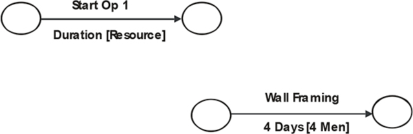
A precedence diagram is based on representing the activities. Activity data is shown within a box, and relates to the activity, as opposed to the node in the case of the CPM method. Consequently, time data is referred to as ‘earliest start date’, ‘latest start date’ etc, rather than ‘earliest event time’, ‘latest event time’ etc. Refer to Figure 2.13.

Time data
Dependencies
The logical links between activities are known as dependencies. These are generally one of the following three types as shown in Figure 2.14, i.e.
- Finish-to-start
- Start-to-finish
- Finish-to-finish
It is also possible, but rare, to have Start-to-finish dependencies.
The dependency may have a time component (shown in the following figure as ‘n’). This is known as ‘lag’. It is also be just a logical constraint.

Start-to-finish dependencies
Note that in all cases the logical relationships between A or B and other activities may well mean that other constraints control the actual start or finish of Activity B, not the dependency between A and B.
Activity constraints
The timing of activities may be constrained by factors unrelated to logical relationships between the activities. By default, analysis assumes that all activities start As Soon as Possible (ASAP type). However, the start or end date for each activity can be controlled by defining the constraint on it. If the activity constraint conflicts with the logical relationships between activities, the activity constraint overrides the logical relationship.
Activity constraints may of the following types:
- ASAP As Soon As Possible
- ALAP As Late As Possible
- FNET Finish No Earlier Than
- SNET Start No Earlier Than
- FNLT Finish No Later Than
- SNLT Start No Later Than
- MFO Must Finish On
- MSO Must Start On
Milestones
Milestones are notional activities introduced into the network to mark particular points, say, completion of each phase (e.g. completion of user definition), or achievement of a critical series of events (e.g. award of a major contract). Milestones are activities with a defined duration of ‘0’ time units. Milestones are typically used to enable higher level reporting and monitoring of the schedule.
Be aware of the fact that a milestone could involve a time-consuming design review that could take several days or weeks, in which case the milestone should be shown with an appropriate duration, or else the preceding design review must be incorporated in the project network diagram.
2.3.4 Analyzing the network
The method of determining ESD, LSD, EFD, and LFD is similar to that for the Critical Path method, although account must be taken of all defined dependency lags as well as activity constraints.
With this method it is necessary to create an artificial ‘Start’ and ‘Finish’ activity, both with zero duration. ESD and EFD are calculated by a forward pass. Calculate the ESD for each activity by consideration of preceding activities:
-
- EFDa plus n (dependency lag) equals ESDb.
The latest ESDb determined from all precedent paths is the ESDb to be used.
-
- EFDb equals ESDb plus duration.
Once the Finish task is reached, the LSDs and LFDs are calculated by a backward pass. Calculate the LSD for each activity by consideration of succeeding activities plus dependencies and durations.
-
- LFDa equals LSDb minus n (dependency lag)
The earliest LFDa determined is the LFDa to be used.
-
- LSDa equals LFDa minus duration
This is not as difficult as it sounds, but some practice is required to master the subtle aspects of more complex networks.
Example
Activity A has no predecessors, and a duration of 4 time periods (e.g. months). Activity B has no predecessors either, and a duration of 3 time periods. Activity C has a duration of 2 time periods and can only start when A is finished. Activity D is expected to take 4 time periods, and can only start when A and B is finished. The following figure shows the completed network. Note the following:
- Each activity is labeled in the middle, and the duration is shown at the top, in the centre field.
- The dummy activities ‘start’ and ‘finish’ have zero duration
Now the forward pass:
- The ‘start’ activity begins and ends at time zero (EST = EFT =0)
- Activity A can begin straight away (EST =0) and ends at time 4 (EFT =4)
- Activity B can also begin straight away (EST = 0) and ends at time 3 (EFT =0)
- C must wait for A. The earliest it can therefore start is at time 4, ending at 6 (EST = 4, EST = 6)
- D must wait for both A and B to finish and can therefore not start before 4, ending at 8 (EST = 4, EFT = 8)
- The project is only finished when D is completed, at time 8
- The ‘finish’ dummy task has zero duration, and therefore starts and finishes at 8 (EST = EFT =8)
Next follows the backward pass:
- The ‘finish’ task has zero duration, therefore its LST = LFT = 8
- Completion of C can now be delayed until time 8 (LFT = 8), so with a duration of 2 its LST is now 6
- There is no slack in C, so its latest times are the same as its earliest times
- Since the earliest D can start is 4, B need not finish before then
- A must finish by 4, otherwise it will delay D
The floats are now calculated as LST minus EFT, or LFT minus EFT, i.e. the bottom number minus the top number on either the left or the right side of each block. The critical path interconnects all those blocks with zero slack. Remember that it is possible to have more than one critical path, and that the critical path may change once the project is under way (see Figure 2.15).

AoN analysis for given example
2.4 Presentation of the scheduled network
Once the EST and LFT for every activity have been determined, the network can be drawn to a time scale. This can be in the form of an arrow diagram (Critical Path method) or a bar chart, or both. Allowable float may be shown. These representations are shown in Figure 2.16.
A time-scaled bar chart is known as a Gantt chart. Probably the most useful representation of the network, particularly for managing the project, is a Gantt chart that contains all logic links between activities.
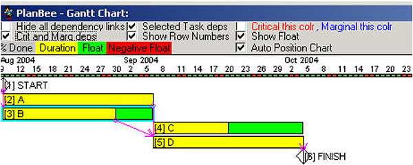
Gantt chart
The following is the result of the AoN analysis, also referred to as a PERT chart (see Figure 2.17).

PERT chart
2.5 Analyzing resources requirements
2.5.1 Resource loading
A highly valuable feature of project network analysis is the ability to generate information regarding the project resources associated with the scheduled activities. In many cases a schedule produced without consideration of the resource implications is meaningless. When reviewing construction schedules for instance, the associated resource data is always required to ensure that the planned inputs are, in fact, practical.
Useful resource analysis requires that the demand for each category of resource be identified separately for each activity. This process can be performed manually, but this can be time consuming. Computer programs used for Critical Path analysis will generally produce charts showing resource loading versus time. These are called resource histograms.
2.5.2 Resource leveling
In some project situations the total level of projected resource demands may not be a major concern, because ample quantities of the required resources are available. It may, however, be that the pattern of resource usage has undesirable features, such as frequent changes in the amount of a particular manpower skill category required. Resource-leveling techniques are useful in such situations because they provide a means of distributing resource usage over time in order to minimize the variations in manpower, equipment or money expended. They can also be used to determine whether peak resource requirements can be reduced without increasing the project duration.
Those activities that have float are rescheduled within the available float to provide the resource profile that is the most appropriate. The available float is, of course, determined by the critical path analysis which has been performed with consideration of resource requirements. During the resource leveling process the project duration is not allowed to increase.
In the case of a single resource type the process of resource leveling can be conducted manually for sizeable networks with the aid of magnetic scheduling boards, strips of paper or other physical devices. However, in situations involving large networks with multiple resource types the process becomes complicated, since actions taken to level one resource may tend to produce imbalances for other resources. In such situations the process can really only be done using a computer.
2.5.3 Constrained resource leveling
The process of resource leveling by rescheduling non-critical activities within the original project duration may not be sufficient if the resource level for one or more resources is limited. Where it is not possible to obtain all resource requirements equal to or less than the available resource levels by this process, it is necessary to extend the project duration sufficiently to allow the required resources to balance the available resources.
This process is called constrained resource leveling. Again, the process can really only be done effectively using a computer, but generally all project scheduling software programs have this feature (see Figure 2.18).

Resource analysis
2.6 Progress monitoring and control
2.6.1 Defining the plan
The effectiveness of monitoring depends on the skill with which the programmer has broken down the project into defined parcels of work. Progress is assessed by measuring the ‘percentage complete’ of individual activities during the project. If it is not possible to assess the true progress (percentage complete) of significant of significant activities, then reporting inaccuracies will be the norm and deviations will be difficult to detect. To reduce or avoid this uncertainty, each activity should be divided into stages, completion of which is both useful and measurable. This breakdown should be finer rather than coarser. Such ‘activity milestones’ must be agreed between the Project Manager and the person responsible for the specific activity at the start of the project.
The importance of this approach can be demonstrated by reference to the two scheduling scenarios shown in Figure 2.19. In each case progress can only be properly measured on completion of each activity.

Two scheduling scenarios
Assume that in both scenarios Activity A is completed one month late, at which time the problem is identified for the first time. Under Scenario I the effective rate of improvement required to complete within the original project duration is 125% (i.e. 5 periods of work outstanding with 4 periods available to complete). By comparison, in Scenario II the effective rate of improvement required to complete within the original project duration is 150% (i.e. 3 periods of work outstanding with 2 periods available to complete).
The project manager has a much greater likelihood of achieving the project time objective in the first scenario.
2.6.3 Monitoring
The project manager must be aware at all times of the actual deviance of the project from the plan. Monitoring and reporting on progress must be regular and accurate. There is no justification for the project manager not to know the precise status of the project.
The objective of the progress monitoring system is to:
- Identify areas of the project where performance is below expectations
- Provide information on such deviations from the project plan in sufficient time for corrective actions to be usefully applied
Most of the available project scheduling computer software programs allow for progress to be ‘posted’, that is, for the current status of programmed activities to be updated on the computer schedule. The network is then re-analyzed to take into account the new data, and new completion dates for the remaining activities are computed. Generally the updated schedule can be compared against an earlier baseline schedule and progress variance, both historical and future, tabulated. This baseline facility is of extreme benefit when monitoring performance.
A typical graphic progress report can provide the information shown in Figure 2.20 for each activity in the schedule.

Progress reporting
The effectiveness of the reporting is a crucial element of the project control function. A reporting format should be standardized for each project, and all progress reporting required conforming to the specified format. To provide effective control the reporting must be:
- Timely
- Accurate
- Easily interpreted
A formal report should include the following information:
- A summary of efforts and accomplishments during the reporting period
- A summary of planned efforts and accomplishments in the following period
- The status of project milestones (achieved and predicted)
- Any changes in milestones status since the previous report
- The consequences of any delays in milestones
- Desired changes in predicted performances
- Actions required/suggested/recommended to obtain desired changes, and their cost/resource implications
- In addition to the text, a graphic progress analysis clearly indicating actual versus planned progress should be included.
Progress monitoring and reporting must be a regular activity; at least monthly on projects over six months, but probably fortnightly or weekly for projects of shorter duration. Remember that the aim of monitoring progress includes the ability to take action that will allow any time lost to be regained. This may not be achievable if monitoring occurs at less frequent intervals than, say, 10 percent of the project duration.
Slippage is commonplace and should be a major concern of project managers. It occurs one day at a time and project managers need to be ever vigilant to keep it from accumulating to an unacceptable level. Slippage can be caused by complacency or lack of interest, lack of credibility, incorrect or missing information, lack of understanding, incompetence, and conditions beyond one’s control, such as too much work to do. Project managers need to be on the alert to detect the existence of any of these factors in order to take appropriate action before they result in slippage.
Project slippage is not inevitable. In fact, there is much project managers can do to limit it. The tools of progress control are the bar charts or critical path networks described above. The project manager should take the following steps:
- Establish targets or ‘milestones’ – times by which identifiable complete sections of work must be completed
- As each target event occurs, compare actual against targeted performance
- Assess the effect of performance to date on future progress
- If necessary, re-plan so as to achieve original targets or to come as near as possible to achieving them
- Request appropriate action from those directly responsible for the various activities
2.6.4 Change control
The project manager must implement a project change control procedure to provide for effective control of discretionary changes during the project, and to track non-discretionary changes. Thus, if a proposed change in scope is requested, the commitment of the change must require specific approval, given only when the cost and time impacts have been defined. In the case of unavoidable changes their impact on the project must be systematically incorporated into the project information system, especially with regard to time and cost changes.
2.7 Software selection
There is a large selection of so-called Project Management software available on the market. The label is a misnomer – the software provides a tool for ‘scheduling’ projects and, in many cases, integrated cost/time management.
This does not constitute a tool with the capabilities to turn the user into an instant project manager. However, effective project management does require the use of appropriate software. The issue here is on what basis the selection of the software is made.
This is relatively simple if the program is going to be used by a number of people within the organization for low-level planning, presentation, and control of relatively simple projects. In that case ease of learning and use becomes the primary criteria. That means, for most people, a Windows-based tool with sufficient single project or multi-project capability.
In the cases where the scheduling program is required for more complex project management functions and where the cost of learning to use the software is not an issue, the basis for the selection will relate to the capabilities of the program required to suit the demands of the particular situation.
The following elements will be relevant to an informed evaluation of the best tool for a particular application.
Essential requirements
These must match the specific requirements for the required application in order to be considered for selection:
- Multi-project capability
- Number of activities per project
- Number of resources per activity
- Resource input capabilities
- Resource calendar options
- Capability to input resource and overhead costs in the form required
- Baseline capabilities for presenting update comparisons
- Presentation graphics capability and flexibility
- Flexibility to tailor cross-tab reports, particularly financial reports
Other considerations
Other issues that will be relevant to the selection include:
- Ease of learning
- Training available
- Hardware requirements
- Product support
Learning objectives
Effective cost management is a key element of successful project management. The history of project management is punctuated by projects that have been financial disasters. These include many high profile projects, where it is reasonable to assume that considerable planning and effort went into the cost management functions. Examples include the Sydney Opera House, the Concorde and the Channel Tunnel.
Many small projects do not have more than superficial attention paid to the implementation of effective cost management systems, but in general the cost overruns on small projects are very high in percentage terms.
The objective of this section is to review the critical aspects of the cost management process that must be properly addressed to ensure effective financial control.
Cost management includes the processes required to ensure that the project/contract is completed within the approved budget. These processes comprise:
- Cost estimating
- Budgeting
- Financial control
- Change control
- Cost monitoring
- Value management
3.1 Cost estimating
3.1.1 Importance of estimates
Estimating costs is of fundamental importance to every project. Estimates are prepared to meet two different objectives:
- As the basis for determining the economic feasibility of a project
- As the basis for cost management of the project.
If the estimates are unnecessarily pessimistic, decisions on project scope are improperly constrained. In the worst case the project, or elements within it, may not receive approval to proceed. On the other hand, if the initial cost estimates are unrealistically optimistic, the resulting project cost objectives are unlikely to be achievable, irrespective of the quality of the project management applied.
3.1.2 Basis of estimates
A cost estimate is a calculation of the approximate cost of a specific project or project component. Contrary to the belief often held by those who approve the budget, the estimate has an inherent uncertainty. The accuracy of the estimate is directly related to the amount of information or detail available at the time the estimate is prepared, the method used to develop the costs, specific inclusions and exclusions, and various assumptions necessarily made. It follows that when the estimate is presented for approval, the basis upon which it has been prepared must be clearly stated. This should include:
Inclusions/Exclusions
It is necessary to specify all inclusions and exclusions; for example fees, contingencies, escalation, principal supplied plant, etc.
Order of accuracy
The order of accuracy must be stated in terms that have specific probabilities defined. For example, in capital works projects the following definitions are commonly employed:
|
-30% to +50% |
|
-25% to+25 % |
|
-5% to +10% |
Cost indices
Where it is appropriate to include for escalation, the cost index upon which the estimate has been prepared must be identified. If the estimate includes provision for escalation, the index calculated to apply at completion must also be stated. The dollar value of the escalation is most accurately determined from a forecast cash flow that determines the value of expenditure, and thus the related escalation, on a quarter-by-quarter basis.
Escalation can only be estimated on the basis of judgment. However, the particular judgment may only be that of the person doing the estimate, or a projection provided by a recognized and competent source.
Contingency
Contingency is an estimate of cost provided against expected, but currently undefined, costs associated with the particular risks of the component being estimated. Contingency levels may be assessed in any of the following ways:
- Judgment based on the cost impact of particular risks, and probabilities of each particular risk arising
- Historical experience of similar activities
- Organizational policies for risk management
- Probabilistic modeling, using appropriate software
3.2 Estimating methods
The estimates for the base cost of the project, or project components, can be developed using a number of different methods, some of which are closely related. The following are the most common.
Resource based estimates
The estimate of project costs is based on a breakdown of the project/contract into work packages. The definition of costs for each package of work is then developed from first principles on the basis of anticipated resource inputs viz. labor, materials, equipment, overhead margins, etc.
Estimating guides
In certain industries, estimating cost data is published frequently for the express purpose of assisting estimators by providing detailed cost data for common standardized elements or components. For example, $ per ton for reinforcing steel used in the construction industry.
Parameter estimates
The cost estimate is developed on the basis of industry cost data for standard parameters, for example the $ per square meter for a structure of a specific type.
Exponent estimating
Exponent estimating is predicated on the assumption that the costs of different sizes of similar items vary according to the relative size raised to some power. In other words:
Cost Item 2 = Cost Item 1 x [Capacity Item 2 / Capacity Item 1]N
Figures for N are published for specific types of equipment, and are valid over a specific range of capacity, such as liters per minute, for a specific type of equipment such as a centrifugal pump. N is typically in the order of 0.6 for elements of a process plant, and this relationship is known as the ‘six tenths rule’.
3.3 Forecast final cost
The concept of defining and tracking project costs with respect to ‘Forecast Final Cost’ (FFC) is the basis for effective cost management.
At the project definition stage the cost estimate should be presented in terms of FFC, where:
- FFC = Base estimate + Contingency + Escalation + Exchange fluctuations
Tracking project costs with respect to FFC is discussed later in this chapter.
3.4 Documentation of estimating procedures
Every organization has a vital interest in ensuring that the estimates used for making investment decisions are prepared on a uniform basis, and have the highest practical level of reliability. This requirement will only be met when the organization has developed and documented appropriate estimating procedures.
Such procedures should include:
- Definition of alternative estimating basis to be applied
- Definition of alternative estimating methods to be applied
- Definition of contingency estimating to be applied
- Sources of data to be used
- Applicable checklists
- Documentation requirements
- Review requirements.
3.5 Budgeting
Purpose
Budgeting involves allocating the cost estimates against the project/contract schedule. The budgeting process should establish a cost baseline that provides:
- The basis against which project performance may be measured
- A forecast payment schedule to allow for funds management by the principal
Where budgets incorporate estimates prepared at different cost indices, the component estimates need to be normalized to a common index.
Management reserve
It is recommended that, subject to a policy on the specific basis for determining it, ‘management reserve’ be included when defining the total budget:
- Budget Total = Forecast Final Cost + Management Reserve
A management reserve is a provision for cost increases arising from unanticipated sources, for instance changes in scope caused by changes in project performance specification. This approach is not essential, but has the advantage that minor changes in project scope can be accommodated without the need to repeatedly return to the Principal’s board for approvals of revised budgets.
It is important to understand the distinction between contingency (provision within the component estimate for expected but undefined cost changes within the project scope) and management reserve (provision within the budget for possible future project scope changes).
Time base for budget
The time base for the budget, i.e. the ‘spreading’ of expenditures over the budget period, is defined by allocating the costs for each component against the programmed occurrence of the activity.
This is achieved directly by the use of appropriate project management software. It is also very common to use spreadsheets to generate the budget cash flow. Depending on the type of project, expenditures can be projected in weekly or monthly increments.
Documentation of budget procedures
Procedures defining the basis for budget preparation should be standardized and documented in the same manner as estimating procedures.
3.6 Financial control
Scope
The definition of financial controls should extend to:
- Controls over the commitment of funds, i.e. financial authority
- Controls over the approval of expenditure, i.e. authorization of payments
Financial authority
The approval of the budget should be differentiated from authority to commit expenditure to that value. Delegation of financial authority to incur commitment within the approved budget should be subject to a formalized process for each component within that budget.
This approach provides the following safeguards:
- The principal maintains full control over the commencement of the expenditure, and the extent of his liability at all stages of the project
- Where more than one individual has responsibility for implementation of the project, their specific levels of financial authority are clearly defined
- Where outside consultants are used to manage contractors, they may be liable to the principal if they commit funds in excess of the delegated level of financial authority
Project procedures should therefore define the procedures applying to the allocation, commitment, and revision of financial authority.
Authorization of payments
Payment of every invoice must be subject to a formal approval by the individual responsible for the particular budget element. Non-compliance with this obvious requirement is common, and often causes problems relating to overpayment of moneys properly owed.
3.7 Change control
The need for change control
Effective change control is a vital element of project cost control. This process is often referred to as scope control.
Following approval of the project budget, there will be unavoidable changes to the project arising from discretionary and non-discretionary sources. For example:
- On an IT project discretionary changes include user requirement modifications, hardware configuration upgrades, etc
- On capital works projects, discretionary changes include scope changes and design modifications, while non-discretionary changes include estimating inaccuracies, site conditions and contractor claims
Every change has a potential impact on project/contract scope, schedule and cost. Approval of discretionary change must follow analysis of the real impact on the project, and assessment of the costs and benefits. The impact of non-discretionary changes must be identified as early as possible to properly inform the project/contract manager of the real status of costs.
Change control procedures
Change control is implemented via a change control procedure that defines how changes are to be initiated or advised, evaluated, and, in the case of discretionary changes, approved.
A typical project change notice is included in Figure 3.1.

Project change notice
3.8 Cost reporting
3.8.1 Reporting requirements
The basic objective of the financial report must be to provide an accurate status report of forecast financial cost versus approved budget. To meet this objective, the financial report needs to include the following information:
- Initial budget
- Approved budget variances to date
- Current budget
- Current forecast final cost
Further useful information includes:
- A breakdown of the difference between the original estimate and the current forecast final cost by scope, estimate and escalation variance
- Trends in the forecast final cost.
Depending on the value to the project team, the following information could also be included:
- Commitments to date
- Accrued expenditure to date. Accrued expenditure arises when contract payments are subject to retentions
- Expenditure to date versus planned expenditure to date. This will be of value if cost and schedule variance are identified using earned value analysis
- Forecast expenditure
3.8.2 Monitoring forecast final cost
Recall that at the project definition stage, the estimate of final cost (i.e. total dollars spent) is forecast as:
FFC = Base estimate + Contingency + Escalation + Exchange fluctuations
With this original FFC identified as FFC0, the revised FFC at subsequent stages of the project is defined as:
| FFCn | equals | FFC0 | |
| plus | Estimate variances | (actual to date + anticipated future) | |
| plus | Scope variances | (actual to date + anticipated future) | |
| plus | Escalation variances | (actual to date + anticipated future) | |
| plus | Provision for changes in exchange rate fluctuation |
3.8.3 Variances defined
Estimate variance
An estimate variance is a change in the estimated cost of an element included in the original estimate. The calculation of estimate variances will include periodic recalculation of the contingency provision since, as work is completed during the execution of the project, the required allowance for contingency will decrease.
Scope variance
A scope variance is a change in the estimated final cost of the project due to the inclusion of a new element that is not within the scope of the defined project, or the deletion of an existing element within the scope of the defined project.
Escalation variance
An escalation variance is a change in the total calculated escalation for the project. As the project progresses, total final escalation costs will need to be updated to take into account the actual movement in cost indices.
3.9 Value management
The purpose of value management
The objective of the Value Management (VM) process is to achieve the lowest possible cost without prejudicing required functionality or necessary quality; i.e. to improve the value/cost relationship. The VM process provides an analysis, generally at a particular point in the design phase, which evaluates the cost effectiveness of the proposed solutions. On larger or more complex projects, a VM study during the brief finalization process is often justified. At a later stage in the project, separate VM studies can be undertaken on the design.
VM is more than a cost review; it is a structured process within which all elements of a design brief and design solutions are tested against a number of parameters, such as what the real functional requirements of each specific element is, and what solution most efficiently meets those requirements. VM has produced some excellent results in many instances. In general, savings and improvements achieved from the VM process will justify the costs involved.
Value management methodology
The VM process includes pre-study activities, the VM study itself, and post-study activities. Pre-study activities, generally undertaken by the VM study leader, include:
- Co-ordination of the study process
- Collection of relevant information and documentation
- Some pre-study review and modeling
The actual VM studies are conducted in the form of workshops. The specific objectives for each study are defined as an initial activity during the workshop.
The participants include the study leader, representatives of the client organization, the designers (this term is used generically), and representatives of the supply, installation and construction functions. At the option of the client, personnel not connected with the design team may be present to contribute a view which is entirely independent of the solutions being reviewed. The process undertaken during the workshop requires that the VM study leader operates as a facilitator. The process, which is both rational and creative, is structured to review operating criteria and assumptions, identify risks and opportunities, and create and analyze alternative solutions.
Learning objective
The objective of this chapter is to set out a basis for risk management that will provide sufficient understanding of the process for implementing effective risk management for a specific project.
All projects have associated risks. The extent to which risks exists for a particular project component determines how sensitive successful project outcomes are to that component. Effective project management requires that, if project outcomes are risk sensitive, relevant risks are properly managed.
The procedures described in this chapter conform to definitions and processes defined in document AS/NZS ISO 31000 : 2009 Risk management – Principles and guidelines.
A detailed review of the analytical techniques necessary to undertake comprehensive quantitative analysis is outside the scope of this chapter. See ISO/IEC 31010, Risk management — Risk assessment techniques
4.1 Definition of ‘risk’
Risk is the effect of uncertainty that prejudices the successful achievement of the project outcome, by adversely impacting on cost, time, or functional objectives.
The elements of risk are:
- The likelihood of the event arising; and
- The consequences if it does arise
The inter-relationship of these elements is shown in Figure 4.1.

Probability-impact matrix
4.2 Risk management
4.2.1 Definitions
The following definitions will be used throughout this chapter (see Table 4.1).
Risk-related definitions

4.2.2 Elements
The main elements of the risk management process are:
- Establishing the context
- Risk identification
- Risk analysis
- Risk evaluation
- Risk treatment
- Monitoring and reviewing
4.2.3 Benefits and costs
The benefits from applying risk management accrue to both the project team and to the project sponsor. These benefits include:
- Providing a more informed basis for committing to the project financially
- An increased understanding of the project, leading to better planning
- Development of more suitable project processes (e.g. contracting arrangements)
- Facilitation of more rational risk taking
- Improving the distinction between good luck and good management
The cost of applying risk management to a project varies, as a function of the scope of the project and the depth to which the process is applied. Costs can be very low (say, a few hours) at one end of the scale, and ranging up to several percent of the total management costs if done in depth and as an ongoing process throughout all project phases.
4.2.4 Application of risk management
Risk management is applicable to all projects. While this may be obvious, it is the widespread experience of project managers that it is difficult to convince clients to adopt comprehensive risk management processes.
While it is clearly of great relevance on large or complex projects, it will provide benefits on all projects except on recurring projects being undertaken in an unchanging environment – if such a situation ever arises.
Risk management is a continuous process that can be initiated at any point in the project cycle, and continued until the costs of maintaining the process exceed the potential benefits. It has the greatest potential benefits if used early on in the project. The following points within a project should be specifically addressed within the risk management processes:
- During the feasibility study – to assist the selection of implementation strategies
- At the time of client commitment – to properly understand the real exposure to risk
- At time of tender – by contracting parties
- Post tender – by the project manager to assess the likely performance of the contractors
- During implementation – to monitor existing and emerging risks and amend and/or develop appropriate management strategies
4.2.5 Documentation
In order to maintain a record to facilitate ongoing reviews as well as an adequate audit trail, all components of the risk management process must be adequately documented.
Sample documentation, based on that recommended within AS/NZS 4360:2004, is appended.
4.3 Establishing the context
4.3.1 General
This defines the external and internal parameters which need to be taken into account when managing risk, and setting the scope and risk criteria for the risk management policy.
The outputs from this step are:
- Definition of the elements within the project to define a structure for the identification and analysis of risks; and
- Definition of risk assessment criteria directly related to the policies, objectives and interests of stakeholders
This process reviews the external, internal and project contexts.
4.3.2 The external context
This analysis reviews the external environment in which the organization seeks to achieve its objectives The purpose is to identify factors that enhance or impair the ability of the organization to manage risks. This includes the financial, operational, competitive, political, legal, social, and cultural aspects of the operating environment.
4.3.3 The internal context
This analysis is directed at the internal environment in which the organization seeks to achieve its objectives
4.3.4 The project context
This analysis is directed to the specific project objectives and its component technologies, activities, timing and physical environment.
4.4 Risk identification
4.4.1 General
The organization needs to identify sources of risk, areas of impacts, events (including changes in circumstances) and their causes and their potential consequences. The purpose of this step is to identify all the risks, including those not under the control of the organization, which may impact on the framework defined above.
A systematic process is essential because a risk not identified during this step is removed from further consideration.
4.4.2 Procedure
The first step is to identify all the events that could affect all elements of the framework.
The second step is to consider possible causes and scenarios for each event.
The process of risk identification can be complex, and a planned approach is necessary to ensure that all sources of risk are identified. This process may involve:
- Identifying the key personnel associated with the project, i.e. those whose understanding of the project environment and the project processes enables them to properly appreciate the sources of risk
- Undertaking structured interviews with these personnel. Checklists should be used to ensure comprehensive coverage of all project elements. The objective is to determine, from each person; concerns, constraints and perceived risks within their area of expertise
- Organizing brainstorming sessions
- Engaging the services of specialist risk analysts
- Reviewing past experiences in this regard
4.5 Risk analysis
4.5.1 General
The objectives of risk analysis are to comprehend the nature of risk and to determine the level of risk. This involves:
- Assigning a level of risk to each identified event
- Providing data to assist the assessment and treatment processes
- Separating minor, acceptable risks from other requiring further consideration
Risk is analysed by consideration of the likelihood and consequence of events occurring within the context of existing controls i.e. management procedures, technical systems and risk management procedures.
The analysis can be carried out to various levels of refinement by way of qualitative and quantitative analysis, or a hybrid of the two. It is necessary to avoid subjective biases when analysing the likelihood and consequences of individual risks.
4.5.2 Qualitative risk analysis
Once the risks associated with every area of the project have been identified, the impacts of these risks are assessed qualitatively. Where the impact that the risks within specific areas have on the overall project may be different, the resulting impacts need to be evaluated independently. All identified risks are categorised into low/high probability, and low/high impact classifications.
Initial responses for the significant risks should be developed at this stage. If risks requiring immediate response are identified, then the initial response should be implemented. A proposed response to an initial risk may result in consequential risks not initially present. These are known as ‘secondary risks’. Secondary risks need to be included in the risk assessment process as they may dictate that a proposed response to a primary risk is not acceptable.
This analysis can be performed with software such as ‘RiskTrak’. The advantage of using software is that it ensures that few questions are left un-asked, and also provides a database with all risks, their assessment and methods of addressing them that can be accessed by the entire project team.
Interviews are conducted in general or specific project. Figure 4.2 shows the interviewing in progress.

Risk interview in progress
(Courtesy RiskTrak)
Once the project-related risks have been identified, their chance of occurring and the related severity of such an occurrence have to be ascertained, together with the method and costs of addressing the issue. This is done via a conventional possibility/consequence matrix as shown in Figure 4.3.
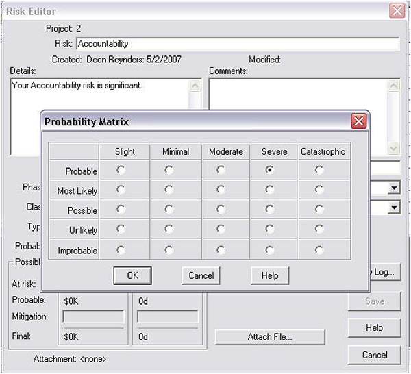
Risk appraisal
(Courtesy RiskTrak)
4.5.3 Quantitative risk analysis
A quantitative risk analysis enables the impacts of the risks to be quantified with respect to the three fundamental project success criteria: time, cost and functionality.
The techniques outlined below have been developed for analysing the effects of risks on the time and cost outcomes of projects, and are in common use. These techniques are well documented in the literature, and a detailed treatment is outside of the scope of this chapter. These techniques are often not applicable to analysing risk impacts on functionality objectives.
Sensitivity analysis
Generally considered to be the simplest analytical technique to apply, this analysis determines the effect on the desired dimension of the project – i.e. time, cost, functionality – from changing each one of the risk variables independently.
The resulting Sensitivity Diagrams – one for each project dimension modeled – identifies impact each variable has on project outcome, and what those impacts are. By inspection, the critical variables are apparent. This provides the opportunity to develop a risk management strategy that targets the most critical risks.
Probabilistic analysis
Probabilistic analysis is an analysis to identify the frequency distribution for a desired project outcome, e.g. total project cost, internal rate of return or total project duration.
The most common form of this analysis uses sampling techniques, normally referred to as Monte Carlo Simulation. This can only be practically undertaken using an appropriate software application package.
A mathematical model of the project is developed, incorporating all relevant variables. A probability distribution is then defined for each variable, and the project model is analyzed taking into account all risks in combination. This analysis is repeated a number of times, typically 100 to 1000 passes, and at each pass the value for each variable is randomly calculated within the assigned probability distribution. The results from each analysis provide a distribution frequency of the project outcome. This establishes a mean outcome, and the range of outcomes possible.
Probabilistic analysis can be performed on cost as well as project schedules. One of the better-known software packages in this regard is @RISK, although there are various alternatives on the market, some stand-alone and others as add-ons for scheduling packages such MS Project and Primavera. An example of an inexpensive software package for Monte Carlo analysis on project costs is Project Risk Analysis. The following figures show the statistical behavior of project costs for a given project (see Figure 4.4).

Project Risk Analysis: Cost distribution (Courtesy Katmar Software)
If the above bell curve distribution is integrated from left to right, it yields a so-called S curve that indicates the possibility that the cost will be less than a given value (see Figure 4.5).

S-curve (Courtesy Katmar software)
From the S-curve (specific values on the X-axis are available via the ‘Statistics’ function) it can be seen that, despite a mean cost of $4978 being predicted, there is only a 50% chance of that happening. In order to guarantee the cost with 99% certainty, provision has to be made for a cost of up to $5395, i.e. a contingency of $417 or 8.79% is required.
An alternative to Monte Carlo Simulation is the Controlled Interval and Memory Method. On less complex analyses this technique offers great precision for less computer effort.
Decision trees
This method has been in use for a considerable time and provides for decision making based on a relatively crude risk assessment. Decision trees display the set of alternative values for each decision, and chance variable as branches coming out of each node. Figure 4.6 shows the decision tree for the R&D and commercialization of a new product.

Decision tree (Courtesy Analytica)
Influence diagrams
This is a relatively new technique, used as an interface with computer based risk models to facilitate development of complex risk models (see Figure 4.7).

Influence diagram (Courtesy Analytica)
Decisions, shown as rectangles with sharp corners (i.e. ‘Fund R&D’ and ‘Launch Product’), are variables that the decision maker has the power to control. Chance variables, shown as oval shapes (‘Success of R&D’ and ‘Market success’), are uncertain and cannot be controlled directly. Objective variables, shown as hexagons (‘Market value’), are quantitative criteria that need to be maximized (or minimized). General variables (not shown here) appear as rectangles with rounded corners, and are deterministic functions of the quantities they depend on.
Arrows denote influence. If ‘Market success’ influences ‘Market value’ it means that knowing the extent of the ‘Market success’ would directly affect the beliefs or expectations about the ‘Market value’. An influence expresses knowledge about relevance and does not necessarily imply a causal relation, or a flow of material, data, or money.
Influence diagrams show the dependencies among the variables more clearly than decision trees would. Although decision trees show more details of possible paths or scenarios as sequences of branches from left to right, all variables have to be shown as discrete alternatives, even if they are actually continuous. In addition, the number of nodes in a decision tree increases exponentially with the number of decision and chance variables and, as a result, Figure 4.6 would need in excess of a hundred nodes to display the decision tree for Figure 4.7, even if we assume only three branches for each of the two decisions and two chance variables.
4.6 Risk evaluation
4.6.1 General
Risk evaluation is used to assist in making decisions based on the outcomes of risk analysis as to which risks need treatment and the priority for such treatment This involves comparing the levels of risks determined from the analysis process against the acceptance criteria previously established.
The output from the risk evaluation is a prioritised list of risks requiring further action.
4.6.2 Categories of risk
The assessment process will determine whether risks may be categorised as low or acceptable, or other.
Low or acceptable risks may be accepted as they are, or with minimal further treatment, subject only to ongoing monitoring.
Risks that fall into the other category are subject to a specific treatment option.
4.7 Risk treatment
4.7.1 General
Risk treatment involves identifying the range of options available for modifying those risks identified as requiring action in the previous stage, evaluating those options in respect of each risk, and developing and implementing risk treatment plans.
Note that some risk response activities may have been undertaken during the qualitative analysis step, if the urgency of developing a response to specific risks warranted it.
4.7.2 Identifying treatment options
Risk treatment options include the following. These options may not necessarily be mutually exclusive, or appropriate in all circumstances.
- Risk avoidance means not proceeding with the activity or situation giving rise to the risk
- Risk taking means taking or increasing the risk to pursue an opportunity
- Risk removal eliminates either the likelihood or the consequences of the risk
- Risk reduction reduces either the likelihood (e.g. by training programmes, QA programmes, preventative maintenance, etc) or the consequences (e.g. by contingency planning, design features, isolation of activity, etc)
- Risk transfer transfers all or part of the risk to another party. Mechanisms include the use of contracts, insurance, and organizational structures (e.g. a joint venture)
- Risk retention can be adopted by informed decision.
There are two additional classifications for risk treatment responses, viz. immediate or contingency.
- An immediate response is one where the project plan is amended in order for the identified risk to be avoided, or its impact minimized
- A contingency response is one where provision is made within the project plan for a contingent course of action that will only be initiated if the risk occurs
4.7.3 Evaluating treatment options
Options generated for risk treatment should be evaluated on the basis of the extent of risk reduction versus the costs of doing so, taking into account the risk assessment criteria previously developed.
Clearly large reductions in risk where achieved for relatively low cost should be implemented. Other opportunities may be less easily justified on economic grounds, including the need to consider rare but severe risks that cannot be economically justified, but which could be fatal if they arose. Some risks provide benefits (e.g. adoption of new technology) that need to be factored into the evaluation.
4.7.4 Developing risk treatment plans
Treatment plans document how the selected treatment options will be implemented. They define responsibilities, time frames, expected outcomes, budgets, performance measures and planned reviews.
Effective implementation of the risk treatment plan, including undertaking the planned reviews, requires appropriate management input on an ongoing basis. This should be addressed within the project planning.
4.8 Monitoring and review
4.8.1 General
Monitoring and review of all elements of the risk management programme is essential.
The specific risks themselves, as well as the effectiveness of the control measures, need to be monitored. Few risks remain static and factors impacting on the likelihood or consequences may change.
Changing circumstances may alter earlier priorities, and factors impacting on the cost/benefit of management strategies may vary. If, following treatment for a specific risk, there is still a residual risk, then the management of that risk needs to be investigated.


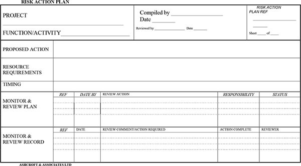
Learning objective
The purpose of this chapter is to:
- Set out some fundamentals concepts and definitions relating to quality and quality management
- Define the components of a quality system
- Review the application of ISO 9000:2005 quality guidelines to the development and certification of quality systems
- Define the components of effective quality assurance in a project environment
5.1 Quality and quality management basics
5.1.1 General
Historically, quality was achieved entirely by reliance on quality control procedures in isolation; that is, by inspections of the product during manufacture, and/or on completion. Uncovered defects involved remedial work, often expensive in terms of time and cost. Not all defects were found before in-service failures occurred. With the increase in complexity of systems and manufacturing processes, the limitations of the historical approach have necessitated a different philosophy. Real evidence of quality in all processes and activities involved in the generation of the output (design, manufacturing, installation and commissioning) must now be demonstrated. Incorporating quality assurance into each of these processes using a systematic approach promotes the reliable achievement of quality objectives.
Quality management is a key issue for many businesses in today’s environment, and many clients rank demonstration of quality management competencies highly when evaluating potential suppliers. The benefits to the purchasers include better quality of services and products, cost benefits due to improved efficiencies within the suppliers’ processes, and lower whole-of-life costs. Suppliers derive competitive advantages from the lower costs as well as from attaining certification to recognized standards.
Achievement of quality is a management function for which responsibility cannot be delegated. If it is to be implemented successfully, the quality program must be seen to have the commitment of senior management.
5.1.2 Quality concepts
Degree of excellence
This refers to the grade of defined product or service, when all quality characteristics are considered as a whole. It is best illustrated by the difference between a luxury sedan and a small utility vehicle, both made to a high standard of conformance in terms of the specified criteria for quality characteristics.
Fitness for purpose
A product or service is fit for purpose if all necessary quality characteristics are present, and it adequately meets (but does not unnecessarily exceed) prescribed or required criteria for each characteristic.
Quality characteristics
Quality is defined or demonstrated with regard to the following criteria:
- Performance – the primary operating characteristics
- Features – secondary characteristics that supplement the primary functional operation characteristics
- Reliability – a measure of the frequency of breakdown
- Conformance – to pre-determined standards
- Durability – a measure of the life span of the product
- Serviceability
- Aesthetics (subjective)
- Perceived quality (subjective)
5.1.3 Quality definitions
The following section will clarify some of the quality-related concepts used in this section.
Inspection and test plan
This is a document that identifies inspection and test schedules (verification activities) and the acceptance criteria for every activity in the process.
Non-conformance
Non-conformance refers to the non-fulfillment of specified requirements (ISO 8402).
Quality
Quality refers to the totality of features and characteristics of a product or service that bear on its ability to satisfy stated or implied needs (ISO 8402). In a contractual situation quality requirements are generally specified. In other situations the needs that are implied rather than expressed must be identified. Needs are normally defined as criteria to be achieved with respect to defined characteristics. In some situations the needs may change over time.
Quality assurance
Quality Assurance refers to all those planned and systematic actions necessary to provide adequate confidence that a product or service will satisfy all requirements laid down by a given quality policy (ISO 8402).
Quality Assurance is not an add-on to a process. Instead, its success depends on commitment to the philosophy of total integration of quality planning and implementation throughout all component activities.
Quality audit
A Quality Audit is a systematic independent examination to determine whether quality activities and related results comply with planned arrangements, whether these arrangements are implemented effectively, and whether they are suitable to achieve the objective (ISO 8402).
Quality Control
Quality Control consists of the operational techniques and activities used to fulfill requirements for quality (ISO 8402).
Quality management
Quality Management is that aspect of the overall management function that determines and implements quality policy (ISO 8402).
Quality plan
A Quality Plan is a document setting out the specific quality practices, resources and sequences of activities relevant to a particular product, service, contract or project (ISO 8402).
Quality planning
Quality Planning, in general, identifies which quality standards are relevant to the project and determines how to satisfy them
Quality system
A Quality System is the organizational structure, responsibilities, procedures, processes and resources for implementing quality management (ISO 8402).
Total Quality Management (TQM)
TQM is an approach for continuously improving the quality of goods and services delivered through the participation of all levels and functions of the organization, in order that fitness for purpose is achieved in the most efficient and cost-effective manner. TQM systems provide company-wide operating structures, documented in effective and integrated technical and managerial procedures, which guide and co-ordinate company activities across administration, marketing, technical, sales, etc.
5.1.4 Quality management fundamentals
Customer focus
The ultimate purpose of the quality system is to ensure complete customer satisfaction with the goods or services provided. Focus on the requirements of the customer at every stage in the process is fundamental to ensuring satisfaction. The customer-supplier relationship is therefore of great significance; every quality system should involve the customer, either directly or indirectly. Customer feedback provides the best inputs from which to define required improvements. The focus on the customer has the following elements:
- Define customer needs
- Convert customer needs into products and/or services
- Determine how well the customer perceives performance of product(s) or service(s)
- Determine what new characteristics will better meet customers’ needs
Process focus versus output focus
Note the earlier definition for Quality Assurance. It is not an add-on to a process. Instead, its achievement results from commitment to the philosophy of the total integration of quality planning and implementation throughout all component activities. Quality is achieved by putting in place a quality system that is intended to ensure that all component processes are subject to appropriate planning and control, not by inspection of the end product to see if it is conforming. In other words, quality is planned into the process, not inspected into the output.
Continuous improvement
The process of ‘continuous improvement’ is an essential element of TQM. This process is one of continually involving all process participants in a team environment, reviewing and experimenting in order to make small changes and innovations in the process. The emphasis is on achieving improvements in effectiveness and efficiency from small-scale changes, as opposed to implementation of large-scale technological or capital investments. Note that continuous improvement is distinguished from radical innovations (as result from such investments.)
The effectiveness of the continuous improvement process is a function of:
- Management commitment to the process
- The skill, knowledge, expertise and creativity of the personnel involved
- The authority delegated to personnel as well as the resources available to them
Involvement of personnel
The contributions and alignment of all company personnel are essential to the viability and effectiveness of any quality program. The level of input from personnel will be directly related to the culture that has been instilled by management. Company personnel should be participants in decision-making processes, and should be considered as ‘expert advisors’ regarding the quality system and its application.
To carry out their assigned roles effectively, personnel need an appropriately documented quality system as the platform, relevant training, adequate resources, and the necessary authority.
Leadership
The successful implementation of effective quality management is directly linked to the actions of a champion, the vision of senior management, and strong leadership. Leadership is essential, and considered by many leading experts to be the most important factor.
Quality management will only be effectively implemented where the chief executive is committed to its success. That commitment is demonstrated by:
- Ownership of the ‘quality vision’
- Communication of the necessity to achieve customer satisfaction through quality management
- Developing a company culture that places importance on implementing that policy
- Implementation of an appropriate structure
- Commitment of necessary resources to the development and implementation of the quality program, including training of personnel
- Delegation of authority to those responsible to put the process in place; i.e. to all personnel
Structure
The ‘Quality Manager’ should report directly to the Chief Executive, i.e. ‘quality’ should not be considered to be a subsidiary grouping within a process or production department. It is reported that in most instances where the implementation of quality assurance has not been effective, a prime cause has been the organizational structure adopted by the company.
Data measurement and analysis
Measurement and analysis of data on an ongoing basis, i.e. quality control, is the process by which achievement of defined quality standards is evidenced, non-conforming products identified, and the requirement for system improvements made evident. The principle of effective quality control is based on the following:
- No manufacture without measurement
- No measurement without records
- No records without analysis (including statistical analysis as appropriate)
- No analysis without feedback and corrective action
Benchmarking
Benchmarking is the process of evaluating company practices against best industry practice. The path to competitive excellence requires that the company implements an evaluation program.
5.1.5 Supply chain relationships
The business process of an organization may be defined in terms of chains and interactions between different activities and parts of the company, whereby customer demands are converted into goods and services that meet those requirements. Each part of the organization has a dual role; that of receiver and supplier, adding value by the processes undertaken. The processes may be classified as internal or external, depending upon whether or not the specific chain is entirely internal to the company, or includes an external supplier or customer (see Figures 5.1 and 5.2).

Quality systems – creating the customers/supplier chain
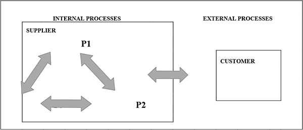
External and internal chains
There needs to be a positive interaction between the internal and external processes at all times; i.e. the customer should be involved throughout.
5.1.6 TQM models
TQM implementation commences with the definition of company objectives, based on an analysis of its strengths and weaknesses, and the desired competitive position. That analysis should include definition of role to be taken by TQM as a means to achieve the defined objectives.
The following models were developed to demonstrate the components of the TQM process (see Figures 5.3 and 5.4).

A component- based TQM model

An action- based TQM model
The elements in each model may be summarized as a component-based TQM model or an action-based TQM model. A component-based TQM model has the following attributes:
- The key: customer-supplier chains
- Systems: documented standards and procedures
- Tools: statistical process controls
- Teams: continuous improvement by teamwork
An action-based TQM model, on the other hand, has the following attributes:
- The key: continuous improvement
- Customer focus: the responsibility of all personnel
- Management commitment: setting goals, establishing systems, allocating resources
- Total participation: inputs of all personnel
- Statistical quality control
- Systematic problem solving: adopting the plan-do-check action cycle, using surveys and customer feedback
5.2 Quality assurance systems
The fundamental platform for Quality Management, in any organization, is the Quality Assurance program, a.k.a. Quality System. This comprises a documented set of policies, organizational structures, systems and procedures serving to implement the quality system of the organization.
The work of Stebbing in developing the framework for systematic quality assurance has become the basis of the modern approach to quality system development. His reference text Quality Assurance – the route to efficiency and competitiveness, [Third Edition] 1993, pub Ellis Horgood Ltd, is recommended reading.
The Quality System consists of the following elements:
Quality policies
This includes the Policy Statement as well as the Quality Objectives of the organization, and the organizational structure and responsibilities.
System outlines
For each significant area of activity of the organization, the various systems or processes that will be subject to quality procedures are defined. The System Outlines include details of which procedures are to be applied in particular circumstances, and associated responsibilities for the procedure application.
5.2.1 Procedures
Detailed procedures are developed for each system element identified in the systems outlines. These procedures should be appropriately detailed, and will generally include reference to quality documents (standard checklists, record sheets, etc) to be completed as part of the process in undertaking the defined procedure.
This hierarchy of a typical Quality System documentation is represented in Figure 5.5.

Quality assurance program hierarchy
The Quality Manual is a document of intent, not detail. The detail is reserved for the procedures.
5.3 ISO 9000:2005 Quality System guidelines
5.3.1 General
The International Organization for Standardization (ISO) has developed quality system guidelines that have gained international recognition as the benchmark for quality assurance systems.
The objectives of these standards are firstly to provide purchasers of products as well as services with independent evidence that the supplier has in place systems to ensure that the desired level of quality will be attained. In addition, they provide suppliers with defined guidelines that provide the basis for implementing a certified quality assurance system.
It may be argued that adherence to these standards will automatically lead to a quality output. This is, unfortunately, not so. While certification of quality system compliance with the relevant ISO standard does mean that an organization is properly applying documented quality systems, it does not mean that those quality systems are necessarily appropriate.
5.3.2 ISO 9000:2005, ISO 90001, ISO 9002, ISO 9003
The ISO 9000:2005 system guidelines recognize differing levels of quality assurance and are applicable in differing situations. There are three levels of quality assurance, defined respectively within ISO 9001, ISO 9002, and ISO 9003.
These standards define quality system requirements in decreasing levels of comprehensiveness.
- ISO 9001– For use where quality assurance is to comply with specified requirements during several stages, which may include design/development, production, installation and servicing
- ISO 9002- For use where quality assurance is to comply with specified requirements during production and installation
- ISO 9003- For use where quality assurance is to comply with specified requirements solely at final inspection and test
Guidance as to the selection of the appropriate standard to apply is set out in ISO 9000:2005.
5.3.3 ISO 9000:2005 quality system elements
ISO 9000:2005 quality systems have a common framework, although the specific requirements vary from ISO 9001 to ISO 9003 and may not be applicable at all levels for a particular organization because of the operations occurring within the organization. The defined quality system elements are set out in Table 5.1.
ISO 9000:2005 quality system elements defined

5.4 Project quality assurance
5.4.1 Project quality management
The generic elements of Quality Management were defined in 2.2 as including Quality Planning, Quality Control, and Quality Assurance. The application of appropriate controls to all elements of the project management processes is, in fact, quality assurance. In other words; project management methodology is a subset of the Quality Assurance Programmes.
The following section addresses the specifics of project quality management as a subsidiary control process directed at ensuring the fitness for purpose of the project deliverables.
5.4.2 Project quality planning
The following are inputs to the quality planning process for a project:
Quality policies
Quality policy refers to the formal policy of the sponsor organization and/or the project management group. This might include, for example, requirements for using ISO 9000 accredited suppliers only.
Project scope statement
This defines the project objectives and major deliverables.
Project process descriptions
This involves the definition of the processes required to provide the project deliverables defined in the project scope statement.
Standards
This involves the definition of specific standards applying to the project. The outputs from the quality planning process are:
- Project quality procedures. These are defined process controls for each process within the project.
- Project inspection & test plans (ITPs). These define the required programme for applying quality controls.
5.4.3 Project quality control
Inputs to the Project Quality Control function are:
- Project Quality Procedures
- Project Inspection and Test Plans
- Inspection and measurement of product/service characteristics
Outputs from this function are:
- Acceptance/reject/rework decisions
- Test documentation
- Adjustments to the process
5.4.4 Project quality assurance
Inputs to the project quality assurance function are:
- Project Quality Procedures
- Project Quality Documentation
The output from this function is:
A Quality Improvement Program – i.e. a program to define and implement revisions to Project Quality Procedures and ITPs.
5.4.5 Project quality procedures
Typically the Project Quality Procedures are organised within three divisions:
Project management
These operate to control the activities of the project team itself, and will typically cover:
- Preparation of Project Quality Plans
- Project control procedures
- Project administration
Design services
These are issued to design consultants and define the requirements for quality systems and procedures to be applied by them. These will typically cover:
- Requirements to produce Project Quality Plans
- Requirements to submit quality system and procedure documentation for review
- Requirements to submit design validation and other test documentation for review
- Processes for ensuring design interfaces are integrated
- Design quality assurance
ITPs may be defined in the scopes of service, or submitted as part of the Project Quality Plan prepared by the consultants.
Supply, installation and construction services
These define the requirements for quality systems and procedures to be applied by suppliers, installers, and contractors. These will typically cover:
- Requirements to produce Project Quality Plans
- Requirement to submit quality system and procedure documentation for review
- Requirements to submit test documentation for review
ITPs may be defined in the contracts, or submitted as part of the Project Quality Plan prepared by the suppliers, installers, and contractors.
The procedures will be the relevant procedures, where they exist, selected from those defined within the Quality Assurance Program of each contributing organization, to be applied on the specific project. Where they do not exist the required procedures need to be specifically prepared.
Learning objective
The objective of this chapter is to:
- Demonstrate the power of applying Earned Value analysis to measuring and predicting project performance
- Develop skill in the application of the Performance Measurement System
6.1 Earned value analysis
Earned Value Analysis (EVA) is the analytical part of what is known as Earned Value Management (EVM), so the two names are often used interchangeably. If the project plan is prepared with a budget linked to the project schedule through activity based costs it is possible, and of considerable benefit, to establish an integrated reporting system that takes account of cost and time deviations.
This provides a management tool that determines the extent of cost variances that may be separately attributed to over/under expenditure and to schedule deviations.
The basic approach is to periodically measure progress and cost in comparable units against a baseline. The units of measurement are usually dollars, although man-hours are also sometimes used.
6.1.1 General
A significant benefit of the EVM approach is that most of the data can be presented graphically, in one macroscopic view of the project progress. Because there is a common basis for these measurements, all individual measurements can be summarized (rolled up) to any level, up to the entire project. Each work item is given a weight factor equal to its planned dollar value or Budget At Completion (BAC) divided by the total of the BACs in any measured grouping.
Because all measurements are based on their dollar value, they can all be plotted on the same graph, with TIME on the x-axis and DOLLARS on the y-axis. Refer to Figure 6.1 for an illustration of the application of EVM.
Figure 6.1(a) depicts a traditional cost report comparing actual expenditure to budget. This does not assist the project manager in determining the status of the project. Superficially seen, expenditure is close to the budget and there would appear to be little cause for concern.
Figure 6.1(b) analyses the same data to provide information on the cost and schedule variances. In this case both variances are negative: the project is behind schedule, and the cost of the work completed is higher than budgeted. Thus the true position is that the project is poised for significant cost overruns as well as time delays.

Typical expenditure: budget

EVM – cost and schedule variance
6.1.2 EVM terminology
At first sight the simplicity of EVM is well-hidden behind the terminology that has been generated. Fortunately it very quickly makes sense to use the acronyms listed in Table 6.1. Note that these calculations can be done for a single item (on the WBS), or for a group of items, or for a rollup (summary) of the entire project. All measurements referred to must obviously be taken at the same time.
EVM terminology defined
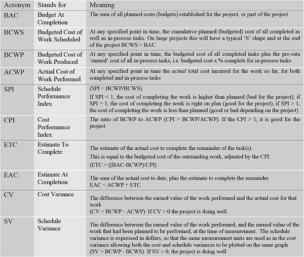
6.2 EVM analysis illustrated
The situation
Suppose it is required to and connect widgets as part of an overall project (i.e. labor costs only). The project schedule is divided into four equal periods. Assume that the schedule calls for the widgets to be connected during the last three periods, with 30 units in period 2, 40 units in period 3, and 30 in period 4.
Assume labor costs of $25 per man-hour and productivity of 0.8 man-hours per connection.
The project plan
The planned costs can be calculated as follows:
| Total labor | = | 100 x 0.8 Mh | = | 80 Mh |
| Total cost (BAC) | = | 80 x $25 | = | $2,000 |
| Unit cost | = | $2000 / 100 | = | $20 |
The planned production schedule is as follows:
| Totals | Period 1 | Period 2 | Period 3 | Period 4 |
| 100 No | 0 | 30 | 40 | 30 |
| 80 Mh | 0 | 24 | 32 | 24 |
| $2,000 | 0 | $600 | $800 | $600 |
Progress evaluation
Assume that it is now the end of period 2, and you are conducting measurements of progress and cost. Your progress measurement indicates that you have completed 20 connections so far (versus the 30 planned).
Because you have to connect a total of 100 widgets, you are now 20% complete with this work item. Therefore you have an earned value (BCWP) of $400 (20% x $2,000).
You have incurred 20 man-hours of labor against this cost code to the end of period 2. Thus you can calculate the costs to date (ACWP) of $500. (20 x $25 = $500)
EVM analysis
Applying the formulae:
- BCWS = 30 x $20 = $600
- BCWP = 20 x $20 = $400
- ACWP = $500
Therefore it is possible to calculate the performance indices:
- SPI = BCWP/BCWS = 400/600 = 0.67 ( <1; not good)
- CPI = BCWP/ACWP = 400/500 = 0.8 ( <1; not good)
The variances can also be calculated:
- CV = BCWP – ACWP. In this example it is $400 – $500 = – $100. The negative value means performance is worse than planned.
- SV = BCWP – BCWS. In this example, it is $400 – $600 = – $200. The negative value means performance is worse than planned. Note that although this is a schedule variance and it is really indicating how far you are ahead or behind in terms of your scheduling for this project, but it is expressed as a Dollar value and hence it can be shown on the same graph as the other variables.
Several formulas can be used to compute the EAC. The answers can be considerably different even though based on the same data, and the answers are equally legitimate.
In this example we might assume that the future is likely to be directly proportionate to the past. Thus since it cost $500 to do $400 worth of work, it will cost $2000/CPI = $2,000/0.8 to complete all the work that is:
- EAC = $2,500.
However, it may equally be valid to assume that future work will be completed at the original planned rate and cost. Some software packages make this assumption. On that basis:
- ETC = 80 x $20 = $1,600, and therefore
- EAC = ACWP + ETC = $500 + $1600 = $2,100
The reality is probably somewhere between the two. In the latter case, where the outstanding work is expected to proceed at the original planned rate, ETC is often expressed as FTC (Forecast To Complete) and EAC is then expressed as FAC (Forecast At Completion). This could be confusing, but the important thing is to understand the concepts behind this and not to become entangled in acronyms.
6.3 Computer based integrated time and cost control
Most commercially available project management software packages provide for integrated time and cost analysis and reporting, to some or other extent. The terminology and acronyms defined above are those normally used.
A simple alternative for smaller projects is to develop a PMS analysis using a spreadsheet. For each scheduled activity it is necessary to enter (say weekly) resource hours budgeted, actual and percentage complete. The spreadsheet can be set up to calculate budgets, planned percentage complete, and the PMS parameters.
See the following example, where progress is analyzed after each of the first four weeks of a six-week program.
This analysis shows that despite budget and actual expenditure being close, there is significant poor performance, in terms of both schedule and cost variances. The trend is improving, but on this analysis time overrun can be anticipated in the absence of specific measures to accelerate the rate of progress, and a cost overrun seems unavoidable.

Learning objective
The success of a project is strongly influenced by the characteristics of the project manager, both as the practitioner of the project management technical skills, and as the leader of the project team.
The objectives of this presentation are to:
- Review accepted theories relating to the key elements of management and leadership
- Identify the personal attributes that influence the effectiveness of the project manager
- Review organizational cultures, and the implications for project management
- Identify key issues relating to the development of effective project teams
- Review the factors that influence the authority and power of the project manager
- Identify responsibilities of the project manager that are the essential elements of the project management function
- Discuss the alternative strategies for appointing project managers
7.1 Management and leadership
7.1.1 Management versus leadership
The role of the project manager is a synthesis of management and leadership.
There is a substantial difference between the two activities. Davis (Human Relations at Work, McGraw-Hill, 1967) defined the difference in the following terms:
“Leadership is part of management, but not all of it. A manager is required to plan and organize, but all we ask of the leader is that he gets others to follow. Leadership is the ability to persuade others to seek defined objectives enthusiastically. It is the human factor which binds a group together and motivates it towards goals.”
Bennis (Good Managers and Good Leaders, Across the Board, 1984) defined the difference as:
“A leader does the right thing (effectiveness), a manager does things right (efficiency)”
The quote above is ‘catchy’ but creates the impression that management and leadership are mutually exclusive activities, and that a good manager is not necessarily a good leader. This is not so. Leading is simply a part of management, along with directing, controlling, planning and coordinating; and therefore a good all-round manager is by necessity a good leader as well.
The opposite is not necessarily the case and history is riddled with examples of great leaders who were marginal or incompetent managers.
7.1.2 Management theories
Classical management theory defines the basic functions of management as planning, leading, organizing, directing and controlling (or planning, organizing leading and controlling). In addition to that, initiating and closing functions arise because of the specific nature of projects.
The basic elements of project management correlate closely to those defined in the classical model of management. The reality is, not surprisingly, that project management cannot be divorced from general management.
There are nevertheless significant differences between the two, and it is generally accepted that management of a project is more demanding than management of an operational environment since the situation tends to be more dynamic. In the final analysis the project manager is responsible for the achievement of defined, measurable project objectives. Project managers will focus their energies on the achievement of those objectives, in some instances with less regard for the sensitivities of the project team members than would be the case in a functional situation.
7.1.3 Leadership theories
Thousands of studies have been undertaken to review the characteristics and traits of successful leaders, and many definitions of the optimum blend of characteristics have been defined as a result. Handy (Understanding Organizations, Penguin, 1981) proposes three groups of leadership theories:
Trait theories
According to Handy, successful leaders tend to have the following learned or inherited characteristics:
- Intelligence. They have an above average intelligence without being geniuses, as well as the ability to identify common themes, solve complex problems and comprehend the work of team members
- Proactive. This refers to the ability to identify the need for action, and the strength of character to initiate the required action
- Self-assurance. They have sufficient confidence in themselves to believe that what they are doing is appropriate
- Helicopter mind. They have the ability to move within different levels, i.e. to understand the detail but without losing the global view
Style theories
Certain types of behavior are more effective for a leader than others:
- Autocratic. The autocratic manager dictates ‘what’, ‘how’ and ‘when’
- Democratic. The democratic manager respects the opinions of the team members, and pursues consultation before making decisions
- Laissez-faire. This type of manager behaves like any other team member, and all team members work on their own
Contingency theories
One of the better-known examples in this regard is the Situational Leadership model (Hersey and Blanchard- Centre for Leadership Studies). This model works very well in dynamically changing situations and is part of the training syllabus for US Army officers (see Figure 7.1).
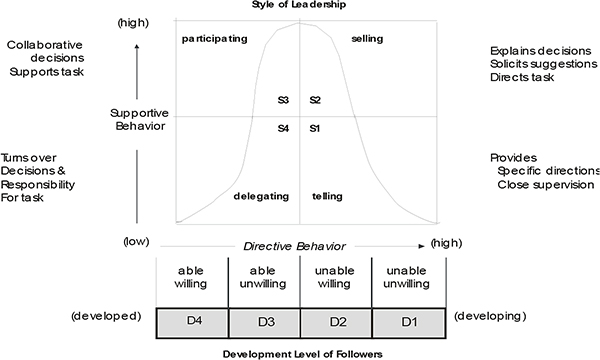
Situational leadership model (Hersey & Blanchard)
In this model the follower can be categorized in one of four categories of ‘readiness’ viz. D1 through D4. Ideally the leader has to respond with the appropriate leader behavior, viz. S1 through S4. In the following discussions, ‘unable’ means technically incapable to perform the task at hand, and ‘unwilling’ means being hesitant or feeling insecure (e.g. because of a lack of relevant experience), or simply having an attitude (motivation) problem.
The behavior of the leader is shown on two axes. The horizontal axis shows the extent of the leader’s task behavior (i.e. directive behavior or degree of guidance to the follower). Towards the left the degree of the leader’s intervention diminishes, while it increases towards the right. The vertical axis represents the degree of supportive behavior (i.e. relationship behavior). It decreases towards the bottom and increases towards the top. The leader-follower relationship can now be summarized as follows:
- D1-S1. The follower is unable and unwilling (insecure/unmotivated), hence requires a leader-directed approach. This is typical of a young graduate joining an R&D team, for example. The leader adopts a ‘telling’ or directive style, making decisions for the follower and providing specific directions and close supervision. The leader is high on directive behavior, but low in supportive behavior. He basically tells the follower (albeit in a ‘nice’ way), what to do and how to do it.
- D2-S2. The follower has now developed and moved on to the quadrant where he/she is still considered technically unable, but willing (confident/motivated). The leader still directs the tasks, but adopts a ‘selling’ style, explaining decisions and soliciting suggestions. The leader is still being very directive (maybe a little less than in S1), but much higher on supportive behavior
- D3-S3. The follower is now able, but unwilling (insecure). This could be expected from a scenario where a member of the project team is, for the first time, appointed as project manager. The leader will adopt a participating style, making collaborative decisions with the follower or allowing the follower to make decisions and then supporting them. The leader is lower on directive behavior than in S1 and S2, and relatively high on supportive behavior
- D4-S4: The follower is now able and willing. The leader can turn over decisions and responsibilities for the task (i.e. delegate the task) to the follower. In this case the leader is low on both directive and supportive behavior as there is no need for either. There are, however, two very important points to consider.
- Delegating a task to a person who is not able and willing to perform the required task is a surefire recipe for disaster
- One can delegate responsibility but not accountability. The leader delegating the task still has to keep a watchful eye over it, as ‘the buck still stops’ with the leader if things go wrong
7.2 Cultural influences on project management
7.2.1 General
The culture of the organization within which the project is implemented, and the culture developed within the project team, have significant impacts on the success of the project management effort. Project managers need to be aware of these influences, how to react to them, and how to modify them.
The following discussion sets out a definition of culture within these environments, identifies the characteristics of organizational cultures, recommends strategies to be adopted by the project manager to operate effectively within those different cultures, and examines the cultural issues arising within the project team. Characteristics of an effective project team are listed.
7.2.2 Culture defined
Smirchich and Stubbart (Strategic Management in an Enacted World, Vol I, Monographs in Organizational Behavior and Industrial Relations, Jai Press, Greenwich CT, 1983) describe culture as:
“The degree to which a set of people share many beliefs, values and assumptions that encourage them to make mutually reinforcing interpretations of their own acts and the acts of others”.
As a result of the system of shared norms, the culture creates shared meanings for the individuals, thus providing bonds between them. The culture creates a social environment that influences the behavior of the individuals. The culture may generate commitment to management values, and will provide a perception of the organization to people within and outside of it.
Culture is transmitted directly, by the communication of beliefs and values, through both formal and informal mediums. It is also transmitted indirectly by way of the organization’s rituals, symbols and myths.
Project managers are normally involved with a number of different organizations, and therefore different cultures, within a single project. The differing organizations comprise the client organization, functional departments within an organization, and the project team itself. The project manager needs to be aware of the differing cultures, and the influence of those cultures, to avoid or minimize conflict and misunderstanding.
7.2.3 Organizational cultures
A useful model of organization cultures has been developed by Cameron (Cultural Congruence, Strength and Type: Relationships and Effectiveness; Working Paper No 401, Univ of Michigan Graduate School of Bus, Ann Arbour, MI, 1984). This model is based on the Jungian framework of psychological functions which states that decision making occurs within any individual on a continuum between thinking (rational, logic based) and feeling (based on whether the particular approach is pleasing or not pleasing), and that information gathering occurs on a continuum between sensing (based on measured or observed values and data) and intuiting (based on feeling). Jung postulated that individuals tend to combine an information gathering preference (sensing or intuiting) with a decision making preference (thinking or feeling) to understand and act on information. The Cameron model is represented in Table 7.1.
Model of organizational culture types

The key to Table 7.1 is as follows: [1] Leadership style, [2] Basis for bonding within the organization, [3] Strategic concerns and [4] Values emphasized.
The characteristics of each type of organization are:
- Hierarchical. The hierarchical culture is very bureaucratic. Individuals look internally for information, and make rationally based decisions. Typically, they build complex administrative systems to regulate their operations. Mining companies often have this type of culture
- Clan. The clan culture emphasizes flexibility in the decision making style, and an internally orientated approach to collecting information on which the decisions are based. An example is Intel
- Market. The market culture is orientated towards the external environment, and typically adopts highly analytical processes in the decision making processes. An example is the U.S. consumer commodities company Proctor & Gamble
- Adhocracy. The adhocracy cultures are flexible in the decision making processes, and are oriented towards the external environment, and are innovative and entrepreneurial. An example is the 3M Company
When interacting with a new organization, or component departments, it is important that project managers identify the type of culture operating. This is necessary in order for them to develop an ‘influence strategy’ that will maximize their ability to obtain the required cooperation and performance. Elmes & Wilemon (Organization Culture and Project Leader Effectiveness, Vol XIX, Project Management Journal, 1988) postulate the following strategies as guidelines.
- Hierarchical. Adopt the bureaucratic approach – i.e. work ‘within appropriate channels’, and adopt precise detailed communications. To gather the required support, look for ‘trades’. It may be useful to appeal to the sense of tradition within many long-lived bureaucracies. Innovation can create obstacles. Conflict resolution is typically avoidance, including postponement. The project manger will assist conflict resolution within this environment by providing a ‘face saving approach’, whereby issues and underlying feelings are expressed without the dispute becoming public. This requires sensitivity and a degree of private communications
- Clan. Focus on consensus building. Create a critical mass of support by involving many key players. Listening, expressing concerns and communicating trust are important if people are to make a commitment. Handle conflicts by collaborative methods
- Market. This culture is highly competitive, and the project manager may need to enable others to see benefits to themselves from project participation. It is useful to attract the support of ‘stars’ within the organization. Competition is a primary means of resolving conflict
- Adhocracy. Adhocracies have weak authority structures, and the project manager needs to be flexible and creative to gain support. Provide participants with freedom and intellectual challenge, and expose them to new problem-solving techniques. Focus on the task should be sensitive. Conflict should be solved by collaborative methods
7.2.4 Creating a team culture
Cultures within the project team are a reflection of the project manager’s preferences and style. The styles of the culture that can arise are similar to those described above. The project manager must ensure that the development of the team culture, and the nature of that culture, is deliberate and planned, not a situation that arises by default.
Mower and Wilemon (Team Building in a Technical Environment, Handbook of Technology, Wiley 1989) describe team building as a process aimed at the development of the team’s task competencies (meeting goals, objectives and targets), and interpersonal competencies (resolving conflicts, developing trust).
Project managers can assist the project teams to reach the desired level of performance in two ways. Firstly, they should protect the team from external conflicts and influences that will disrupt it, thereby interfering with progress towards the desired objectives. This is important where the culture of the dominant organization imposes values, rules or procedures which impede the ability of the team to complete their tasks. Secondly, project managers build up the effectiveness of the team by the values that they transmit to team members. Again, values are transmitted formally via such means as training manuals, meetings and structured discussion, and informally or symbolically.
Project managers need to specifically address the following:
- Clarifying roles, responsibilities and levels of authority for all team members
- Setting up effective channels of communication with all team members
- Setting realistic performance expectations for each team member
- Delegating effectively (instead of over-supervising)
- Publicly rewarding good performance
- Acknowledging legitimate concerns and conflicts within the team
Team building progresses through a series of defined phases to ultimately reach a high level of sustained performance. In the first stage, team members develop an understanding of the project objectives, their roles and responsibilities, and of each other. In the second stage, team members form a definitive view of their importance to the team and the project. During this stage conflicts between team members commonly arise. In the third stage the conflicts have been resolved and the members of the team are able to focus on execution of the project. In the final phase the team members evaluate what has been learned from completion of the task. At each stage the project manager can communicate values that move the team to the next stage.
The stages in team development are referred to as the processes of ‘forming’, ‘storming’, and ‘norming’.
7.2.5 The effective project team
The focus of the project manager is to develop an effective project team. Culture is an important component of this parameter, but it is not the sole issue.
Mower and Wilemon have identified the following characteristics of the effective project team (see Table 7.2):
Characteristics of effective project teams
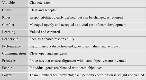
7.2.6 Team motivation
There are certain issues that spur on individuals within the team to even greater achievements, and other issues that stifle performance. For a start, the project manager should ensure that his leadership style when dealing with a specific team member is in line with the degree of readiness of that individual. This will differ from individual to individual, and from task to task. It is not hard to imagine that inappropriate styles such as leaving a newcomer to sort out things for herself (S4 style with an R1 follower) or trying to prescribe to an individual to whom a task had been delegated (S1 style with an R4 follower) can lead to friction and loss of motivation within the team.
There are, however other issues that affect individual performance, sometimes within the ambit of the project manager’s control, and sometimes not. Herzberg has studied the topic and arrived at a list of so-called motivators and hygiene factors. A motivator is a cause for satisfaction, while a hygiene factor is a cause of dissatisfaction. An interesting observation from the results of his studies is that the lack of a motivator does not automatically make it a hygiene factor (de-motivator) and vice versa.
From the following figure it is evident that the major motivators are (in descending order of importance):
- Achievement
- Recognition
- Work itself
- Responsibility
- Advancement
- Personal growth
The absence of these factors, though, do not create an commensurate level of dissatisfaction.
On the other hand, the major hygiene factors are:
- Company policy and administration
- Supervision
- Relationship with supervisor
- Work conditions
- Salary
- Relationship with peers
As with the motivators, it is evident that the absence of a de-motivator does not automatically motivate the individual.
A few interesting observations are that a sense of achievement and recognition for work well done are by far the biggest motivators, while poor administration and unsatisfactory supervision are the greatest reasons for unhappiness. A lack of enough salary is, to a lesser extent, a de-motivator but sufficient salary is not much of a motivator (see Figure 7.2)!

Herzberg’s motivators and hygiene factors
7.3 Authority and power of the project manager
7.3.1 Authority of the project manager
The authority of the project managers directly impact on their capability to perform the role effectively. That authority is derived from the following sources:
- Organizational. This refers to the authority vested in the individual by the corporate structure and policies, the individual’s position within the organization, and the formal delegation of authority from superiors
- Project. This is authority arising from the terms of reference for the specific project, and the manner in which the project organization has been structured and the control mechanisms defined
- de Facto. This is authority arising from the personal and political skills of the individual, and the influence those skills have on allowing the individual to obtain a significant role in the communication process and decisions paths within the project.
The level of authority required by the project manager is variable, and dependent upon the level of accountability that the project manager is held to. Generally the project managers should have more authority than their responsibilities dictate.
Common causes of problems within projects that arise from authority issues include:
- A lack of formal authority
- Incorrect perception of authority (often because of inadequate documentation)
- Dual accountability of individuals. This underlines the importance of having a single point of authority (the project manager) and defined assignment of responsibilities for all team members
- Inappropriate organization structures
7.3.2 Power of the project manager
Power comes from the credibility, expertise and decision making skills of the project manager. Power is granted to the project manager by the project team as a consequence of their respect for performance in those areas.
7.4 Required attributes of the project manager
The specific attributes of effective project managers may be stated as follows:
- Project managers must be proactive
- Project managers must be inquisitive and persistent
- Project managers must have sufficient understanding of the technology related to their specific projects to be able to evaluate the quality of the information provided
- Project managers must to be able to rationally and realistically analyse the current position of the project, to identify principles and trends behind the superficial realities
- Project managers must have the ability to adjust their focus between the detailed plans and schedules, and the wider milestones and objectives. To concentrate on one view at the expense of the other invites disaster
- Project managers must to be able to select appropriate corrective actions when actual performance is not conforming to the plan. This includes generating contingency plans as a common practice
- Project managers must have the ability and confidence to make decisions, and to direct others to implement them once made. In some situations it will be preferable to implement decisions that, while not perfect, are adequate and can be adapted as the circumstances dictate, rather than wait for all information before making a decision. Paralysis by analysis must be avoided
- Project managers require good communication and negotiation skills. It is essential that project managers maintain effective communications at all levels across the project. Within the project team itself, the project manager must be able to motivate, negotiate, resolve conflicts, and persuade. A blend of assertiveness, conciliation and measured aggression is required
7.5 Essential functions of project managers
The following functions are essential elements of the project manager’s role. The appointed project managers must ensure that they are, in fact, fulfilling their responsibilities in these areas.
- Preparing and being responsible for the project plan. Preparation of the project plan is the first opportunity for the project manager to show leadership. It is a very critical step, being the key to all parties involved having a common understanding of objectives, constraints, responsibilities and interactions
- Defining, negotiating and securing resource commitments. Project managers should define, negotiate and secure commitments for the personnel, equipment, facilities and services needed for their projects
- Managing and coordinating interfaces. Projects are typically broken into sub-projects and activities that can be assigned to individuals or groups for accomplishment. Whenever the main project is broken down this way, project managers must manage and co-ordinate the interfaces that are formed by subdividing the work
- Monitoring and reporting progress and problems. Project managers are responsible for reporting progress and problems on the project to the client, and for organising and presenting reports and reviews as necessary. The project manager is the ‘focal point’ for the team, and should be seen as such
- Advising on difficulties. Occasionally a project manager finds that the only way to overcome problem situations is to get help from outside the project. Suffering the difficulty in silence will not be rewarded. The project manager’s management and client must be alerted so that other resources can be brought to bear, constraints can be relaxed, or project objectives can be adjusted. It is not sufficient just to mention the difficulty in passing. The discussion must be an overt act and should be confirmed in writing. If the management or customer agrees to take specific action to resolve the difficulty, that should be in writing as well
- Maintaining standards and conforming to established policies and practices. Project managers must set and maintain the standards that will govern the project staff members, or ensure conformity with established practices
- Developing personnel. It is the project manager’s responsibility to ensure that the staff involved on a specific project has the range of skills necessary to accomplish the task. Where this requires development of existing skills, the project manager must identify the need and arrange for the necessary training to be provided.
7.6 Selection of the project manager
7.6.1 General
Given the consequences of the appointment, the project manager selection requires to be carefully considered, and must not be just an arbitrary action.
The primary issue in making a specific selection is what criteria should be applied to evaluate the suitability of a potential project manager. Technical project management skills and knowledge base requirements are covered elsewhere in this course. The preceding discussion defined specific skills and competencies required of the project manager as an effective leader.
There is a view that the definitions of a good project manager as outlined in this chapter are of limited application, given the reality that the choice of an individual must be made from a very limited group, amongst which there will not be one whose profile closely matches the desired ‘super person’. This view is not acceptable. While that reality may generally apply, it is still highly relevant for the potential employer to be well-informed as to the essential and desirable characteristics required of an appointee.
There are a number of approaches that can be adopted to procure a project manager. These include:
- In-house selection
- Recruitment
- External consultant
Each approach has specific issues, discussed below.
7.6.2 In-house selection
Selection of an in-house individual for the role of project manager has obvious advantages including:
- The appointee’s familiarity with the organization, its culture, procedures and personnel
- The relative ease with which the appointment can be organized
- The ability to make the position only part-time if dictated by the workload of the project management function
Whether or not this option is practical depends upon a number of factors:
- The capacity of the personnel within the organization to accept the additional workload created by the promotion of the incumbent
- The skills and experience of the potential incumbent to undertake the management of the particular project
It must be recognized that only a minority of people have the potential to be effective project managers. However, those individuals will only make good project managers if they have the opportunities to learn and develop the skills and techniques required.
7.6.3 Recruitment
Recruitment is an appropriate option where there is sufficient ongoing work to justify the additional increase in staffing. It has the benefit of allowing the necessary skills to be acquired at a lower cost than employing consultants, and widens the range of potential appointees to be considered for the position. It can have an advantage of providing the opportunity to transfer skills within the organization, but may be better achieved through formal training using external consultants or trainers.
7.6.4 External consultant
The use of external consultants allows specific expertise to be employed without increased establishment costs. The skill levels and experience retained in this way will normally be higher than by recruitment. The external consultant should have industry exposure, but may not have experience with the organization, although this may or may not be considered a critical factor. It is likely that the costs for undertaking the service will be higher than the other options, but on a true hourly rate cost the differential may easily justified. Where the management function is complex because of the nature of the project, or the project is a large one with significant consequences for non-achievement of objectives, this approach deserves serious consideration.
Selection of the consultant should focus on the nominated individual, rather than the company under consideration. Evaluation criteria for selection should include:
- Relevant experience with projects of a similar type and scope
- Previous performance in achieving project objectives
- Personal attributes of the consultant
- Adequacy of standard control procedures to be applied
Providing it is relevant and practical, the engagement of external consultants should provide for a transfer of knowledge to the client organization.
7.6.5 Project managers to avoid
The following personality types do not make effective project managers, and should be avoided.
- The technocrat. The individuals are so concerned and involved with the detail of the technology that they don’t have the time, ability, or desire, to manage the project effectively. They are unable to delegate the performance of the tasks, and commonly lack the interpersonal skills necessary to build an effective team
- The bureaucrat. This refers to an individual who is more concerned with the administration of the project than actually achieving the desired results. Ensuring that the way in which the work is done conforms to the prescribed procedures is seen as more important than the quality or effectiveness of the effort
- The salesman. This is the individual who accomplishes little, but directs his efforts to presenting the project as being successful
Learning objective
The purpose of this chapter is to review selected issues of contract law, where a basic understanding of the applicable law is likely to be of direct assistance to personnel involved in the administration of procurement contracts. The issues addressed in this chapter include:
- The basis of Commonwealth law
- The essential elements of contracts
- Procurement strategies
- Tendering
- Vitiating factors, i.e. those factors that reduce or remove the legal force of the contract
- Termination of contracts
- Extensions of time
- Remedies available for breach of a contract
- Penalties and bonuses
This chapter reviews a wide area of law, and of necessity does not treat each issue in depth. The subject matter is both complex and under continual modification. The information provided is not intended to be relied upon in a specific situation in the absence of professional advice.
Contract law differs from country to country, even amongst Commonwealth countries. Readers are therefore encouraged to familiarize themselves with the latest developments in contract law in their own countries and also in those of their foreign trading partners.
Despite some differences, there is also a remarkable degree of similarity between the contract laws in different countries, partly due to the efforts of UNIDROIT, the International Institute for the Unification of Private Law. UNIDROIT is an independent intergovernmental organization with its seat in Villa Aldobranini in Rome, and has 61 member ‘States’ including Australia, Canada, China, South Africa, the UK, and the USA. It was set up in 1926 as an auxiliary organ of the League of Nations, and following the demise of the League it was re-established in 1940 on the basis of a multilateral agreement, the UNIDROIT Statute. Its purpose is to study needs and methods for modernizing, harmonizing private and, in particular, commercial law as between States and groups of States.
8.1 The Commonwealth legal system
8.1.1 Basis of the legal system
Constitutional basis of law
In the Commonwealth legal system the Legislature makes the laws, the Executive administers the laws and the Judiciary decides in the case of disputes or transgressions of the laws.
Legislation is the body of rules that have been formally enacted or made. Many bodies have the power to lay down rules for limited purposes, for example, social clubs; but fundamentally the only way in which rules can be enacted so as to apply generally is by Act of Parliament. In constitutional theory, Parliament is said to have legislative sovereignty and provided that the proper procedure is followed, the statute passed must be obeyed and applied by the court. The judges have no power to hold an Act invalid or to ignore it, however unreasonable or ‘unconstitutional’ they may consider it to be.
Local government
Some of Parliament’s legislative functions are delegated to subordinate bodies who, within a limited field, are allowed to enact rules. Local authorities, for instance, are allowed to enact by-laws. However, local authorities can only do this because an Act of Parliament has given them the power to do so.
Civil law
The purpose of civil law is to be compensatory and not punitive as in criminal law. The principal divisions are contract and tort. Civil law is based on precedent, and has as the outcome financial award and sometimes mandatory order.
Actions under contract are based on breach of an agreement intended to be binding entered into by parties wherein an offer is made by one, accepted by another, accompanied by some valuable quid pro quo.
Actions under tort are based on breach of a legally recognized obligation owed by one party to another, or to persons generally.
8.1.2 Doctrine of precedent
Binding precedents
The decision in a previous case is binding under the following circumstances:
- It comes from a higher court in the same hierarchy
- There must be an essential statement in the legal decisions (ratio decidendi). The ratio decidendi (the reasoning vital to the decision) is the statement by the judge of the facts he regards as ‘material’, the legal principles which he is applying to these facts and why. The judge may at the same time discuss the law relating to this type of case generally, or perhaps discuss one or two hypothetical situations. These are known as obiter dicta (other comments) and while they may have persuasive force in future cases, they are not binding.
- Material facts must be the same. A material fact is one where it can be reasonably argued that the presence or absence of the fact affects the result.
Persuasive precedent
Precedents in the following cases exercise a varying degree of persuasion.
- Decision from a higher court in another hierarchy
- Court of similar or lower status in the same hierarchy
- Statement of law was beyond that necessary to decide the legal principle, that is, obiter dictum
- The ratio decidendi was distinguishable on the facts
8.1.3 Natural justice
Any breach of natural justice will set aside a decision of the court or the arbitrator.
The elements of natural justice are:
- He who alleges must have proof
- There must be no bias on the part of the judge/arbitrator
- The judge/arbitrator must have no interests in the case
- The other party must be present to argue the case unless he has given his (not his lawyer’s) express consent in writing
8.2 Elements of contracts
8.2.1 Types of contracts
Simple contracts
The contract may be oral, or written, or implied by conduct of the parties.
Formal contracts
Any simple contract put into writing with adequate particulars becomes a formal contract. It is then a formal simple contract.
When made by a company it is generally under seal. The period of limitation is 12 years for breach of contracts made under seal. In respect of building construction contracts, S91 of the Building Act 1991 sets the period of limitation at 10 years.
A contract made by deed must be under seal. If made by deed, no consideration is required, for example, a will or arbitration agreement.
Contract of record
Confined to the legal system, for example, to jail if fine not paid.
8.2.2 Essential requirements
The essential requirements for a contract to be legally enforceable are:
- The intention to create legal relations
- Agreement (offer and acceptance)
- Consideration
- Definite terms
- Legality
- Capacity of the parties
8.2.3 Intention to create legal relations
Unless the courts are satisfied that the parties intended this agreement to be legally binding, the courts will take no notice of it.
8.2.4 Agreement
The courts must be satisfied that the parties had reached a firm agreement and that they were not still negotiating. Agreement will usually be shown by the unconditional acceptance of an offer.
Offer
The offer must fully define the intended agreement. It can be accepted at any time unless:
- It is withdrawn, and the offeree advised
- It is rejected
- A counter offer is made
- There is a fluxion of time, i.e. the offer lapses unless accepted within a reasonable time
If the offer is not withdrawn by A, they are bound to take B’s acceptance. An offer can be made to another person, another party, a specific group, or the world at large. An example of an offer to a specific group is to people who send in coupons. The offer can be made to the world; contracts then exist with those who accept. A relevant case in this regard is Carlill v Carbolic Smoke Ball Co 1892.
It is necessary to distinguish between a genuine offer and ‘mere puff”, or boast, which no one would take too seriously. Note the difference between an offer and an invitation to treat. An advertisement for a tender is normally an invitation to treat. The tender itself is the offer. Refer to Pharmaceutical Soc v Boots 1953 as well as Fisher v Bell 1961.
A tender to supply as required is a standing offer to be converted to contracts upon placement of each order. It can be revoked at any time provided no order is currently unfulfilled.
It is held that advertisement of an auction is an invitation to treat only. Auctions can be called off after advertising. The auctioneer may withdraw the offer to sell up till the fall of the hammer if it is a reserve auction. If it is a no reserve auction, it is held to be an offer to sell to the highest bidder, and the highest bid must be accepted.
An estimate can be an offer. Revocation of the offer must be communicated to the offeree (Byrne v van Tienhoven 1880) and communication need not be by the offeror (Dickinson v Dodds 1876).
An offer may be conditional, and terms as such may be implied. For example, an offer to buy a car is implicitly conditional upon the car remaining in the same condition as when the offer is made.
In general, an offer can be revoked at any time before it is accepted. Note the position regarding tenders as discussed elsewhere in this chapter.
Acceptance
There must be some positive act of acceptance and mere silence will never be enough. Refer to Felthouse v Bidley 1863. Acceptance must be communicated to the offerer.
A contract is completed when the acceptance is posted. Note, however, that the courts accept that letters can be lost in the post.
A counter offer and a mere enquiry must be distinguished from each other. A counter offer destroys the original offer. A mere enquiry does not destroy the offer. Note that an acceptance relying upon a change in terms would be a counter offer. In this regard, refer to Hyde v Wrench 1840 and Stevenson v McLean 1880.
Acceptance should generally be in the same form as the offer, that is, a letter in response to a letter.
An offer must be accepted in the terms of the offer if such terms exist and if they are very precisely defined.
Conditional acceptance is not acceptance. For example, “… subject to a formal contract”, “… subject to solicitor’s approval”. Note, however, that “subject to finance” is held to be binding acceptance.
A provisional agreement pending a later contract is held to be binding.
8.2.5 Consideration
English law will only recognize a bargain, not a mere promise. A contract, therefore, must be a two-sided affair, each side providing or promising to provide some consideration in exchange for what the other is to provide. Consideration is defined as an act or forbearance of value, or the promise of such, for which the same is bought from another. Note that not all promises are deemed to constitute consideration.
Valid consideration includes:
- Executory consideration – when the consideration is a future act
- Executed consideration – when the consideration is the performance of the act (for example, return of dog for reward advertised).
Consideration need not be adequate, that is, the promises need not be of equivalent value. Consideration must exist and have some value otherwise there is no contract. The following have no value and cannot therefore constitute consideration so as to render a contract actionable:
- Past consideration (see Roscorla v Thomas 1842)
- A promise to perform an existing obligation to the promise (see D & C Builders Ltd v Rees 1966)
- A promise made to a third party
8.2.6 Terms of the contract
General
It must be possible for the courts to ascertain what the parties have agreed upon. If the terms are so vague as to be meaningless, the law will not recognize the agreement. There can be no contract at all if it is not possible to say what the parties have agreed upon because the terms are too uncertain. In particular, this will be the case where parties have still left essential terms to be settled between them: they are still at the stage of negotiation, and an agreement to agree in future is not a contract.
This rule is subject to some qualifications. The parties will be bound:
- If, although the agreement is not complete yet, the parties have made provision to render it complete without any further negotiations between themselves (for example, by reference to an independent arbitrator)
- If the parties have agreed criteria according to which the price can be calculated, or have had previous dealings similar to the present transaction, the courts can use these matters to ascertain the terms of the contract.
- If only a fairly minor term is meaningless, it may simply be ignored, and the rest of the contract treated as binding.
Establishing the terms of the contract
The terms of the contract are generally established by an analysis of the contract documents. Some terms may be implied. These simple statements can, in fact, give rise to complex issues.
Contract documents
The law is that the contract will consist only of those papers etc. forming the contract documents. It is therefore essential to include in the bound documents not only the conditions of contract, specifications, drawings and letters of offer and acceptance, but all correspondence between the parties that has a bearing on the bargain agreed to. All included documents must be listed. It is recommended that a conformed set of documents be prepared. All agreed changes to the tender documents should be incorporated directly into the contract conditions, specifications, etc. rather than relying upon an original document with an accompanying wad of correspondence.
Interpretation of contract documents
The court will always presume the parties have intended what they have, in fact, said. The words of the contract will be construed as they are written. A judge has said that “one must consider the meaning of the words used, not what one may guess to be the intention of the parties”. The law requires the parties to make their own bargain, and will not construct a contract from terms which are uncertain. In trying to ascertain the intention of the parties, the contract must be considered in its entirety. Where more than one meaning of a specific section is possible, the reliable interpretation is that which is consistent with the other sections of the contract. Despite any other interpretation the words or grammar may be able to support, if the intention is clear from the context of the document it is pointless to pursue an alternative construction.
In a construction document comprising general and special conditions, specification, schedule and drawings, it is important to define the priority of the documents within the special conditions. This avoids the situation where the Contractor claims to be entitled to rely upon the wording in the schedule only when preparing his/her tender.
The Contra Proferentum rule
This rule means that where a term of the contract is ambiguous, it will be interpreted more strongly against the party who prepared it. Application of this rule is subject to the general principle that a term will not be interpreted against the professed intention of the parties. It will only be applied when other methods of interpretation fail.
Implied terms
Where a term is not stated expressly, but is one which the court considers the parties must have intended to include in order giving the contract business efficacy, the term may be implied. For a term to be implied the following conditions must be satisfied:
- It must not contradict an express term of the contract
- It must be reasonable and equitable
- It must be necessary to give the contract business efficacy
- It must be so obvious “it goes without saying”
- It must be capable of clear expression
Pre contract negotiations
The law will not usually take into account pre-contract negotiations in interpreting the contract. It will not presume that the intentions of the parties prior to executing the contract were not altered by that time.
Representations
Representations are statements made by the parties which induce the formation of contract, but do not form a term of it. If a representation turns out to be false, the remedy lies in an action for misrepresentation.
8.2.7 Legality
Two classes of contracts not enforceable at law because of their content being distinguished [Reference Cheshire & Fifoot’s Law of Contract 6th Ed]. Examples of the first class, illegal contacts include:
- An agreement to commit a criminal offence or a tort
- A contract to defraud the revenue
- Immoral contracts
- Contracts to impede the course of justice
The second class includes contracts that are in breach of public policy (e.g. restraint of trade) or statute but do not involve reprehensible actions. These contracts are invalid and unenforceable, at least to the extent of the offending provisions.
8.2.8 Capacity
A contract will not be enforceable where one of the parties does not have the legal capacity to enter into it. This may arise as follows.
Minors
Capacity of minors to enter into contacts is limited, and subject to specific laws of the relevant country.
Corporations
The doctrine of ultra vires means that corporations, including trading and non-trading, can only exercise the powers provided for within their Articles of Association. In theory all else is ultra vires and contracts entered into in this manner are void. This doctrine is, however, subject to significant exceptions.
In theory contracts made by a corporation must be under seal to be enforceable. There are exceptions which provide for such things as routine minor contracts (e.g. for power etc).
Persons of unsound mind and drunkards
A registered mental patient may not enter into a contract. Contracts may be made on his/her behalf by the courts or receivers appointed for this purpose.
If a person makes a contract while temporarily insane, or drunk, the contract is avoidable if he can prove that he was so insane or drunk at the time as to be incapable of understanding what he did, and the other party knew this. The contract will be binding unless it is avoided within a reasonable time of regaining sanity or sobriety.
8.3 Procurement strategy issues
8.3.1 General
Consideration of the appropriate strategy should include the following factors:
- Risk preferences of the Principal
- The requirement to demonstrate a competitive process
- The need and/or ability to properly define scope of work prior to commencement
- The need or ability to exercise control over the operations of the Contractor
- The need to achieve early completion
There are a number of separate aspects to be considered when determining construction procurement strategy. These include:
- Tendering strategies
- Pricing strategies
- Timing strategies
- Contract types
- Delivery strategies
For the sake of clarity the following discussion treats each option as an independent component. However, the options may be interrelated in some instances such that not all can necessarily be combined: for example, a fast track contract cannot normally be let on a lump sum basis. The options can be subdivided: there are four recognized design build scenarios, and a similar number of cost plus contracts. Thus there are a very large number of different alternatives that may be potentially available when contemplating construction procurement strategies.
8.3.2 Tendering
Tenders may invited be by way of the following mechanisms:
- Public advertisement
- From parties who pre-qualify following public advertisement to do so
- By direct invitation to selected Contractors (including the option of only one)
Public advertisements generally attract all-comers, and while demonstrably ‘open’, create inefficiencies for both the party inviting the tenders, and Contractors.
If ‘public invitation’ is required, the preferred approach is to invite Registrations of Interest publicly, and then limit the tenderers to those clearly meeting pre-qualification criteria. In specialist areas, or where a high standard of performance is sought, tenders should be invited only from parties well-qualified by previous track record. In that case a direct invitation to tenderers known to meet the criteria is expedient.
The basis of evaluation of tenders has a significant impact on project outcomes. Tender evaluation criteria cover a range of issues, i.e. experience, track record, management systems, price – clearly the relative weighting given to each criteria should be given specific consideration in every instance.
8.3.3 Pricing
Pricing may be established either by competition or by negotiation. It is generally possible to get satisfactory tenders by the process of negotiation providing the type of work is well known to the party calling tenders, but competition is clearly the preferred option to arrive at the best tender.
8.3.4 Timing
For supply and services contracts, the contract for the supply or services may be:
- Once off , i.e. a defined output
- For a fixed period, e.g. for 12 months
- A standing order, i.e. for the supply as and when required over a fixed period, generally with a minimum quantity
Timing options for construction procurement contracts include:
- Sequential (i.e. conventional: documentation completed, tender, then supply /installation /construction)
- Concurrent (i.e. fast tracked: supply/installation/construction commencing prior to completion of full documentation)
Clearly the first option provides greatest certainty from the Principals’ perspective, i.e. it has the lowest risk. Fast tracking is necessary to reduce the total time frame for project implementation, and is justified in many cases. There are a number of options available to maintain a high degree of competitiveness in the pricing process on fast tracked projects, e.g. progressive tendering of sub-contract packages.
8.3.5 Contract type
Construction contracts may be one of the following three basic types, or a combination thereof. Contracts of each type may or may not be subject to cost escalation: if not, they are described as ‘fixed price’ contracts.
Lump sum
Under this form of contract, the Contractor/supplier undertakes to do all of the work required for the sum stated in its tender. This means that irrespective of the inputs actually necessary to properly complete the works defined in the contract document, the Contractor is entitled to be paid only the contract sum.
Measure and value
Under this form of contract, the Contractor/supplier undertakes to do all of the work required at the scheduled rates stated in its tender. On completion the amount of work actually done is measured, and payment is made at the scheduled rates for this quantum of work. This contract type is often referred to as a ‘schedule of rates’ contract.
Cost plus
Under this form of contract, the Contractor/supplier undertakes to do all of the work described in the contract, for which all costs are recovered, plus a fee. There are a number of options for the form of the fee, for example: the fee may be fixed, or a percentage of the cost, or subject to a formula based on the proximity of the final cost to a target cost.
8.3.6 Delivery strategies
The selection of the delivery strategy, as defined below, may have significant implications for the Principal. Therefore the implications of each option need to be properly understood, and selection based on consideration of the organization’s strategic operating policies, and in particular the risk management parameters. Selection of the preferred form will be, in part, based on the organization’s competencies and experience.
For service delivery contracts the principal delivery strategies are:
- Defining service requirements based on inputs to be provided. For example, maintenance services may be defined by specifying periods at which specified servicing of plant will be undertaken
- Defining service requirements based on performance and condition criteria for serviced units. For example, maintenance services may be defined by specifying plant operating reliability parameters (e.g. mean time between failures of 2000 hours, or 99% availability) and condition rating parameters on completion of the contract
For construction procurement, delivery options include:
- Conventional (i.e. separate designer and main Contractor)
- Design build. Options range from engaging of a design/build company in the first instance (to undertake all functions from brief finalization through concept development, design and construction), through the recent approach of novation of the design consultant. In this option the Principal engages a design consultant to finalize the brief and develop the concept design, at which point the design consultant’s contract is novated to the selected Contractor, for whom he is responsible to complete the detailed design.
- Management (either management contracting or construction management), defined as follows:
- Management Contracting. The Principal enters into separate contracts with a designer and a management Contractor, who enters into sub-contracts with works Contractors
- Construction Management. The Principal enters into separate contracts with a designer, a construction manager, and works Contractors
An option for all types of contract, i.e. services, supply, or construction, is partnering. There are two approaches.
- Single contract partnering. The partnering agreement is in addition to, but does not modify, the contractual agreement. This provides an enhanced communication framework with the objectives of improving relationships in general, and imposing a dispute resolution process. That process requires matters in dispute to either be settled at a particular level within a defined time frame or the matter is automatically taken up by the next level of management. It is yet to be demonstrated that the single contract partnering model will resolve substantial disputes with major commercial implications.
- Strategic partnering. It is not uncommon in the USA and UK for client and supplier organizations to form strategic partnering alliances. In that case the parties make a long term commitment to work together over many contracts. The contractual provisions become less important as parties seek to avoid disputes in order to maintain the longer term commercial benefits. It is claimed to provide significant benefits to both parties.
The particular delivery strategy adopted will reflect the particular project, the relevant expertise of the Principal and its advisors, and the abilities and prior performance of participating Contractors/vendors. There are many and varied opinions on the relative merits of each approach, often reflecting the interests of the particular party, but some of the innovative approaches are considered by experienced practitioners to have definite merit – e.g. design build by novation.
8.4 Tendering
8.4.1 Compliance with tender procedures
The law relating to tendering practice is in a process of change as the result of recent case law developments, primarily in Canada. It may be assumed that in due course these cases will be followed throughout the Commonwealth. Previously it was generally regarded, at least by the practitioners, that no contractual obligations arose prior to acceptance of a tender.
In Blackpool & Fylde Aero Club v Blackpool Borough Council [1990], tenders were called to operate a concession. A condition of tender was that the Principal would not consider late tenders. The plaintiff’s tender was submitted in time, but the tender box was not emptied at the correct time. When the tender was found it was not considered on the basis that it was late, and another tender for a higher price was accepted. It was held that the Principal, because of the condition of tendering, was under an obligation to consider all conforming tenders submitted on time.
Canadian cases have established further the principle that the conditions of tender must be properly followed by the Principal.
In Ben Bruinsma v Chatham [1995], tenders were called for a civil works contract. After calling tenders it was decided to delete some of the works. This resulted in the tenderer whose price was initially the lowest no longer remaining so, and the contract was awarded to another. It was held that the Principal was bound to select the lowest price based on the documents as originally tendered, or to recall tenders for the varied scope of work.
In Megatech Contracting Ltd v Regional Municipality of Ottawa-Carleton [1989], the instructions to tenderers required that the names of proposed sub-Contractors be supplied. The lowest tender, which was accepted, did not include these details. This tender was significantly lower than the second lowest. The second lowest tenderer sued on the basis the Council had not complied with the instructions to tenderers. The court rejected this argument, relying upon further provisions of the instructions; that “the Corporation reserves the right to reject any or all tenders or to accept any tender should it be deemed in the interest of the Corporation to do so” and that tenders “which contain irregularities of any kind may be rejected as informal”. Note that a Principal is, in general, under no obligation to consider only conforming tenders.
In Chinnok Aggregates Ltd v District of Abbortsford [1990] the instructions to tenders included the provision that “the lowest or any tender will not necessarily be accepted”. The Council had a policy, not disclosed to the tenderers, of preferring local Contractors provided the price penalty was less than ten percent. A local Contractor was awarded the contract, and the lowest tenderer sued. It was held the Council was in breach of an obligation to treat all tenderers fairly.
8.4.2 Revocation of tender
In Canada at least, it is now established law that a tender may not be withdrawn where there is a condition of tendering that tenders shall remain irrevocable for a specified period. This is true even where there is a mistake in the tender.
This approach does protect a Contractor from the risk of sub-Contractors revoking their tender.
8.5 Vitiating factors
8.5.1 General
Contracts can be:
- Void: The contract is defective in law, a nullity; e.g. an immoral contract
- Avoidable: The contract is binding, but one party has the right, at his option, to set it aside
The following factors make contracts void or avoidable:
- Mistakes
- Misrepresentation
- Duress and undue influence
8.5.2 Mistake
Mistake as to facts, but not to general legal propositions, will prevent a contract being enforceable where the apparent agreement in fact lacks true consent between the parties. The general provisions relating to the effect of mistakes are set out below. Note, however, that in a number of Commonwealth countries specific Acts have been passed to address this issue, and the remedies available.
The general principle is that a mistake of fact may prevent the formation of a contract, providing the mistake has an element of mutuality that is the contract was entered into under the influence of:
- A unilateral mistake, i.e. one party influenced by a material mistake known, or ought to be known, to the other party
- An identical bilateral mistake (‘common’ mistake), i.e. the parties are influenced by the same mistake
- A mutual bilateral mistake (‘mutual’ mistake), i.e. the parties are influenced by different mistakes about the same matter of fact or law
A mistake on the part of one party only as to motive or purpose, or with respect to the real meaning of the provisions of the contract, is not sufficient grounds for the contract to be voided.
The mistake must exist at the time the contract is made. If third parties have acquired rights or possessions subsequently and lawfully, i.e. prior to the contract being found to be avoidable, those rights and possessions will generally be retained.
8.5.3 Misrepresentation
A representation is a statement of existing or past fact which does not form part of the contract. A misrepresentation is grounds for rendering a contract avoidable only if it was intended to, and did, induce a party to enter into the contract. The injured party must have been aware of the representation and taken it into account. It need not have been the only inducement.
Note that opinion must be distinguished from fact. If the opinion is not honestly held on the facts, then it becomes a misrepresentation. There are the following classes of misrepresentations.
- Innocent Misrepresentation. An innocent statement made by a party who believed it to be true when it was made and when the contract was entered into. If the representor subsequently finds his statement to be incorrect, or the facts change, he is under a duty to advise
- Negligent Misrepresentation. An incorrect statement made without dishonesty by a party with no reasonable grounds for believing it to be true (Hedley Byrne v Heller & Partners 1963)
- Fraudulent Misrepresentation. A statement made dishonestly, knowing it not to be true, or recklessly, not caring if it be true.
- Non-disclosure. Non-disclosure of a material fact, i.e. mere silence, is generally not misrepresentation. (Note that half-disclosure may be misrepresentation.) It does, however, constitute misrepresentation in three instances:
- Where silence distorts a positive representation
- Where the contract requires uberrima fides i.e. utmost good faith
- Where a fiduciary relationship exists between the parties, i.e. a relationship of trust
The general remedy available to an innocent party where there has been a misrepresentation by the other parties include rescission (cancellation of the contract), or damages in the case of negligent or fraudulent misrepresentations.
8.5.4 Duress and undue influence
Duress refers to actual violence or a threat of same. The threat must be illegal. Undue influence generally, but not necessarily, involves parties in special relationships, and contracts of gifts obtained without free consent.
8.6 Termination of contracts
8.6.1 General
The contract is discharged when the obligation ceases to be binding on the promiser, who is then under no obligation to perform. This arises from:
- Performance
- Agreement
- Passage of time
- Frustration
- Repudiation
- Determination
- Operation of law
8.6.2 Performance
When all obligations under the contract have been fully performed by each party, all obligations are at an end; the contract is said to be terminated by performance. Note the following:
- For entire contracts, complete performance is required before any obligation to pay
- For divisible contracts, payment is required for partial performance
- If performance was prevented by one party, then the innocent party may recover under quantum meruit
Generally complete performance of the obligations created under a contract is required to bring the contract to an end. However, in order to allow the Principal to have timely possession of the works, it is general practice in the construction industry to provide for Practical Completion. That is the point at which the works are substantially complete apart from minor defects. A Certificate of Practical Completion must be issued for each separable portion. Certification should be conditional on the receipt of all maintenance documentation, as-built information and the like
In most installation contracts there is provision for a defects liability period to follow the date of Practical Completion. Where not provided for in the General Conditions of Contract, it is recommended that the Special Conditions should provide for the original defect liability period to recommence from the date of repair where significant faults are identified, in respect of the repaired elements only.
8.6.3 Agreement
This requires new consideration for the agreement, or for the agreement to be made under seal. In an executory contract where there has been no, or incomplete, performance, the mutual release of the parties is consideration, and is called bilateral discharge.
Where the contract has been wholly executed on one side but not the other, consideration is required for the agreement, unless under seal, and is called unilateral discharge. These situations are known as ‘accord and satisfaction’.
Where discharge by agreement takes the form of a new contract, this is called novation.
8.6.4 Time
In common law, time is held to be of the essence, even if it is not so stated, in the absence of contrary provisions. In equity, it is not necessarily of the essence if that view does not result in an injustice.
If time is of the essence, failure by one party to complete their obligations within the time specified allows the innocent party the right to rescind the contract. If time is not of the essence, the continuing failure of a defaulting party to complete within a reasonable time may be evidence of repudiation, and give the innocent party a basis to rescind the contract.
8.6.5 Frustration
A contract may be discharged under the doctrine of frustration if a later event renders its performance impossible or sterile. This event must arise externally and must make the intent of the contracting parties unobtainable, and does not include mere inconvenience or hardship. Reliance cannot be placed upon a self-induced frustration.
Note that the court may imply a continuing condition as a term of the contract (e.g. the health of a party), or the non-occurrence of some event.
The contract is discharged as to the future and both parties must fulfill their obligations as they are due.
Law is now governed by the Frustrated Contracts Act 1944. This Act makes advance payments less expenses incurred before the time of discharge recoverable.
8.6.6 Repudiation
Repudiation occurs when one party intimates by word or conduct that he does not intend to honor his obligations under the contract. Under the Commonwealth legal system, unless modified by specific laws, the common law position is that repudiation arises when one party is in breach of a ‘fundamental term’ of the contract, i.e. such a breach is by itself evidence of an intention not to be bound. Such terms are called ‘conditions’, and differentiated from other terms known as ‘warranties’ breach of which gives rise to a right of damages only as a remedy.
Where a party repudiates the contract does not necessarily come to an end. The defaulting party is in effect making an offer to the other to discharge the contract. In these circumstances the innocent party has the option of refusing or accepting the offer.
If the innocent party makes it clear that he refuses to discharge the contract, the contract stays in force with all future obligations intact. He is under no duty to mitigate his losses, but must not aggravate the damages. This principle is, however, subject to the limitation that it will not apply where the innocent party has no substantial interest in completing performance rather than claiming damages.
If the innocent party elects to treat the contract as discharged he must make this decision known to the defaulting party, and he may not then retract it. The defaulting party remains liable in damages for the breach that led to the default, and any earlier breaches, but is excused from all future obligations.
8.6.7 Determination
In general either party may be justified in determining the contract where the other party has repudiated the contract, i.e. demonstrated a clear intention not to perform the obligations arising under the contract.
Other grounds that justify the Principal determining the contract may be set out in the contract conditions. In these situations, this action should be considered with extreme reluctance, and never initiated without considered legal advice.
The law is particularly severe on Principals who determine a contract. If the basis for the determination is not absolutely in conformance with the contract provisions, or the procedures not followed absolutely without fault, the Principal is most likely to find himself/herself in a serious position that will translate into significant costs. It is necessary that, despite specific clauses in the contract to the contrary, the Contractor be given formal and specific warnings, and to the full extent practical be given the opportunity to rectify the default.
8.7 Time for completion and extensions of time
8.7.1 Time for completion
The date for completion of the contract should be defined in the contract. It is usual to be defined by a particular contract duration which, together with any extensions of time, is added to the date of possession of the site, thus determining the due date. It is not uncommon for construction contracts to provide for staged completion, that is the Contractor is required to hand over the defined separable portions at different times. Each separable portion may also have different dates for possession of site.
In a construction situation time is said to be of the essence if performance by the stated date is essential to the contract. In those instances, failure of one party to complete his/her obligations by the due date is a sufficient basis to release the other party from any obligations under the contract – e.g. payment. Reference within a normal construction contract to “time being of the essence” is almost certainly incorrect, and would not be sustained by the courts. It would only be applicable in the situation where the Principal was providing a facility, such as a temporary concert venue, that would be of no benefit if not complete before the date for the concert performance.
8.7.2 Provisions to extend the time for completion
In general, events will arise that delay the progress of the Contractor. The terms of the contract may define who takes the risk of delays arising from specific circumstances. For instance, the Principal generally accepts the risk of delays arising from industrial disruption, but may not accept the risk for bad weather unless it is extreme.
Contract conditions generally include provision for the Engineer to grant extensions of time for those circumstances where the risk is not to be assumed by the Contractor. Many believe that these provisions are provided for the benefit of the Contractor. This is correct to a limited extent, but the primary purpose of such clauses is to ensure that the Principal is able to retain his/her right to recover liquidated damages. In the absence of such clauses there could be sufficient justification to make time at large, thereby removing the Principal’s right to do so. When time is put at large the only obligation on the Contractor is to complete in a reasonable time. In the absence of flagrant non-performance the Principal could have difficulty to successfully recover damages for a significant delay.
If the Principal is in breach of the contract as a consequence of which the Contractor is delayed, the completion date is set at large, in the absence of express provisions in the contract providing for the Principal to extend time for such a breach. Therefore contracts should provide for the Principal to extend time for completion for such things as failure by him/her to give possession of site by the due date, and delays in providing information, materials and services. If the Principal is to be adequately protected, the wording must specifically define the particular breach that arises. The law will construe extension of time clauses very strictly against the Principal, because they are in effect penal provisions. So a generalized provision, for example “to extend time in the event of special circumstances arising which are beyond the control of the Contractor”, will not be allowed to protect against a breach on the part of the Principal.
8.7.3 Determination of extensions of time
In deciding if there is a justification for granting a particular time extension it is necessary to answer two questions:
- Has the Contractor been delayed by the particular circumstances, thereby becoming entitled to an extension of time?
- What is a ‘fair’ time extension?
To answer the first question it is necessary to determine whether or not the actual circumstances affected an operation on the Contractor’s critical path. This introduces the question of programs. It is not sufficient for the Contractor to show that delay arose on the critical path of some plan of work set out in a program – it must affect his/her actual critical path. The Contractor must be able to prove the progress he/she would have actually made had he/she not been delayed, not the progress he/she said he/she would make, or intended to make. A program is not conclusive evidence of the progress he/she would actually have made. To assist their case, some Contractors fail to supply updated programs, or supply programs that are over-optimistic. It is therefore necessary to exercise vigilance in requesting program updates, and to review the adequacy of the assumptions regarding resource levels and productivity.
To determine a ‘fair’ entitlement it is necessary to determine whether, in the circumstance, a delay could reasonably be minimized or avoided by either rescheduling affected operations, or by introducing additional resources. Although the introduction of additional resources is not a normal expectation, there will be some circumstances where that could reasonably be expected.
The question of concurrent causes of delay is a fertile area of debate. A useful direction is provided by Abrahamson: Engineering Law and ICE Contracts. 4th Edition at page 139:
“The situation where there are concurrent delays, only one of which is outside the Contractor’s control, is most difficult. The case may arise where the Contractor, due to his own deficiencies, is late in reaching a position to start some programmed activity, but in fact could not have started the activity earlier even if he had been ready because of delay by the engineer with some necessary drawings. It is suggested that in this sort of situation the net point is that the Contractor has not in fact been held up by “delay” outside his control, and it is immaterial that if his progress had been different he would have been so held up. The late drawings are not an actual “cause of delay” within this clause. The Contractor therefore is entitled to an extension of time only so far as the drawings are withheld past the date on which he in fact became ready for them.”
“Alternatively, the Contractor may say that if the employer’s concurrent delay had not occurred, he would have been able, for example, to increase his resources or bring pressure on a recalcitrant sub-Contractor so as to overcome the delay for which he is being held responsible. It does not seem that the mere existence of that abstract possibility is sufficient Unless the Contractor raises the issue at the time and gives evidence of readiness and ability in fact, a later argument that his delay would have been eliminated or shortened but for the employer’s concurrent delay is unlikely to be believed by the engineer or an arbitrator on a claim to extension.”
Commonly, clauses within the standard Conditions of Contract refer only to extensions of time. There is no provision for the Engineer to reduce the contract period, for instance if some element of the work is omitted from the contract. This also means that the Engineer cannot simply aggregate variations that include both additional work and deletion of work, to conclude no entitlement to a time extension arises. If any one or some of the variations give rise to an extension of time, that extension must be granted.
8.7.4 Notification of the time extension
The Contractor is, typically, required to apply for a time extension promptly, following the circumstance that causes the delay having arisen. While very late claims might be considered with some skepticism, it is recommended that the supervisor does not rely upon the lateness of claims to refuse an extension of time which is otherwise justifiable.
The law requires that, if the Contractor is to remain subject to the sanction that liquidated damages will be deducted for late completion, he/she must be advised as soon as possible of any extended date for completion. What this means is subject to the specific circumstances. The following references are a good guide.
- Smellie: Building Contracts & Practice 2nd Ed, page 219: “Furthermore, and depending on the construction of the contract, it may be that the extension of time must be made at the time the extra works are ordered, and if made later will be ineffective. And further, the person given power under the contract to extend the time will probably have no power to fix, as an extension of time, a date which has already passed.”
- Page 222 “Extensions of time may be granted even after the works have been completed if the cause of the delay operates until the completion. But if the cause of the delay has ceased to operate before completion, a purported extension made after completion is invalid.”
- Justice Roper in Fernbrook Trading Co Ltd v Taggart [1979] “In my opinion no one rule of construction to cover all circumstances can be postulated and the best that can be said on the present state of the authorities is that whether the completion date is set at large by a delay granting an extension must depend upon the particular circumstances pertaining. I think it must be implicit in the normal extension clause that the Contractor is to be informed of his new completion date as soon as is reasonably practicable. If the sole cause is the ordering of extra work then in the normal course the extension should be given at the time of the ordering so that the Contractor has a target for which to aim. Where the cause of the delay lies beyond the employer, and particularly where its duration is uncertain then the extension order may be delayed, although even there it would be a reasonable inference to draw from the ordinary extension clause that the extension should be given a reasonable time after the factors which will govern the exercise of the engineer’s discretion have been established. Where there are multiple causes of the delay there may be no alternative but to leave the final decision until just before the issue of the final certificate.”
Another consequence of a failure to extend the time for completion at or close to the time the cause of the delay occurs, is to run a serious risk that the Contractor will succeed with a claim for constructive acceleration.
8.7.5 Acceleration
In the absence of special conditions allowing it, the Supervisor has no power to request an acceleration. This provision should be included in the special conditions on significant contracts. Such clauses should allow for an acceleration to be ordered as a variation to the contract with the agreement of the supervisor and the Contractor. It is recommended that the basis of payment be agreed prior to the acceleration commencing in every case.
8.7.6 Payment arising from an extension of time
Where there is provision for additional payment to apply where there is an entitlement to an extension of time, there is often a lot of difficulty reaching agreement on the sum to be paid. Such difficulties can be avoided by the following approach. For the situation where the entitlement to a time extension arises, it can be appropriate to provide for additional sums to be paid on a per-day basis. Instances where this can usefully apply include delays arising from ordered variations, exceptional weather conditions, and delays caused by the Principal. The sum should be nominated in the tender, and be specified as the sole compensation for such delays, deemed to include all onsite and offsite overheads and profits.
8.8 Remedies for breach of contract
8.8.1 Damages
Damages for breach of contract are governed by two considerations, namely the remoteness and the measure of damages.
Remoteness of damages
The test was established in Hadley v Baxendale 1854. The damages must be those either
- Arising naturally, in the normal course of actions, or
- To have been in the contemplation of the parties at the time they made the contract as being the consequence of the breach, that is, whether the special circumstances were within the actual or constructive knowledge of the defaulter at the time of the contract
This rule was developed in Victoria Laundry v Newman 1949 (abnormal profits not foreseeable). It is not the measure which must be foreseeable, but whether the probability of its occurrence was in the reasonable contemplation of the parties.
Measure of damages
The innocent party must be returned to the position it would have been in the absence of the breach, and the measure of the damages is assessed at the time of breach. The plaintiff must take all reasonable steps to mitigate loss caused by the breach. The burden of proving failure to mitigate rests with the defendant.
8.8.2 Liquidated damages
The contracting parties may agree as a term of the contract the amount to be paid in the event of a specific breach. This sum is either a liquidated damage or a penalty. Refer to Section 8.9. Liquidated damages must be a genuine pre-estimate of loss caused by the nominated breach. If the breach arises, the innocent party is entitled to recover the liquidated damages, without having to prove the actual loss.
8.8.3 Extinction of damages
The right to an action for damages may be released by:
- Release under seal
- Release by accord and satisfaction
- Fluxion of time, i.e. the right to claim damages is extinguished by the passage of time. The general law is that the right to seek action for breach of contract is limited to 6 years from the date of the breach, or 12 years if the contract is under seal
8.8.4 Specific performance
A decree of specific performance constrains a contracting party to perform that which it has contracted to do. The remedy is equitable in origin and is only decreed where the common law remedy of damages would be inadequate (for example, the sale of land). It is not a matter of right but is exercised at the discretion of the court (that is, it would not be applied if an injustice would result).
The plaintiff must not be in breach of his own undertakings. This remedy is not available for contracts of service. Damages may be (and, except in the cases involving property, generally will be) awarded instead of specific performance by the court.
8.9 Liquidated damages for late completion
8.9.1 Liquidated damages
Because of the difficulties that arise to establish the real damages or losses resulting to the Principal from late completion of a contract, it is common practice for the damages to be liquidated. That is, an agreed sum is provided for in the contract to be paid as damages for that specific breach. The sum is generally specified on a daily or weekly basis. It does not matter whether or not the actual loss suffered by the Principal turns out to be more or less than the specified damages, the sum specified is the amount of damages to be paid, provided it remains enforceable.
To be enforceable the sum set as the liquidated damages must be a genuine pre-estimate of the probable losses that the Principal will suffer, calculated at the time the tenders are called. In the event of arbitration or litigation it will become necessary to prove that the sum has been calculated properly on that basis. It is therefore essential to keep on file a signed and dated calculation setting out the basis of the calculation. The sum becomes unenforceable if found not to be a genuine estimate prepared prior to issuing the tender documents, or to incorporate a penalty.
Tenderers will normally make provision in their prices for the risk of delays, and costs thereof. Where the level set for liquidated damages is high, this will be reflected in the prices. For that reason liquidated damages are often graduated, with initial levels set at an amount significantly lower than the loss calculated. It is common to prescribe an upper limit on the liquidated damages, either as a nominated total sum, or as a percentage of the contract sum.
Where there are separable portions with differing completion dates, liquidated damages will normally be applied to each stage. It is important to ensure that the cumulative damages that arise in the event of concurrent delays do not exceed the estimate of maximum loss.
Take care where a pro forma schedule is used for the Special Conditions. If the space for the nominated figure for liquidated damages is left blank it is taken to mean that there is no provision for liquidated damages. If however the space contains “-” or “nil” it will be interpreted as meaning zero (specifically $0.00) damages apply in the event of late completion.
8.9.2 Application of liquidated damages
Liquidated damages apply to delays beyond the due date for completion. Therefore if the contract completion date can be demonstrated not to apply, which may be the case for any of the reasons discussed, then liquidated damages cease to be applicable. Where time is at large and the Contractor fails to complete in a reasonable time, the liquidated damages will apply from delays beyond the date fixed as ‘reasonable’.
If the contract provides for the Principal to deduct liquidated damages as and when they become due from payments otherwise due to the Contractor, then in the absence of some further undertaking by the Contractor the Principal will lose the right to recover the damages accrued if he/she fails to deduct them. This is not the case where the contract includes a provision for the Contractor to pay the damages in addition to the Principal’s right to deduct them.
8.10 Penalties and bonuses
8.10.1 Penalties
A penalty is a sum in the nature of a threat to secure performance. Courts will not enforce penalties.
Where the amount stated in the contract as liquidated damages is found to be a punitive sum, i.e. a sum not being a genuine pre-estimate of the probable damages or losses to be suffered by the Principal, but merely a sum fixed to ‘terrorize’ the other party to perform, the Principal will be unable to recover the stated amount as of right under the liquidated damages provisions.
Courts will compensate a party trying to enforce a penalty only to the extent of actual damages suffered. In the case where actual loss exceeds the nominated sum, the plaintiff may sue for breach of contract and receive full damages. This option does not exist where liquidated damages exist.
If the actual damages exceed the stated penalty the Principal can seek to recover the total costs by suing for breach of contract rather than enforcement of the penalty.
8.10.2 Bonuses
Building contracts may provide for a bonus to be paid, for example for early completion, or for completion below a defined price.
In this case, if there is a breach of the contract by the Principal that prevents the Contractor from achieving such completion, recovery of the bonus may be allowed as damages for the breach. So, again, the contract will need to be very carefully drafted.
The effect of variations ordered on the Contractor’s right to the bonus needs to be addressed. It need not be the case that an extension of time provision will necessarily extend the date for which the bonus is achieved.
9.1 Work breakdown structures
9.1.1 Exercise 1
Objective: The objective of this exercise is to develop an understanding of the structure and purpose of Work Breakdown Structures.
Working in groups of two, develop a WBS for a project of your choice. Choose a project with which you have some experience or with which you can at least relate to. Define your project in such a way that it is not too complex, due to time limitations. The following examples might help:
- Building a small experimental aircraft
- Restoring a vintage car
- Building a prototype sailing dinghy for production purposes
- Adding a double garage or small barn to your property
HINT: Most technical people find this a challenge, but try to limit your work packages to about 8 to 10 for this exercise. It may look more impressive with 20 or 30 but you will need too much time for subsequent scheduling exercises built around your WBS.
9.2 Time management
Objective: The objective of the following three exercises is to develop expertise in the preparation of critical path networks using the precedence method.
9.2.1 Exercise 2
Run the spreadsheet ‘activity on node.xls’. You may have to enable macros on your computer. This exercise is self-explanatory and will guide you through the process of calculating start/finish times, calculating floats, and identifying the critical path(s).
9.2.2 Exercise 3
Using a project planning software package such as Plan Bee, create the PERT and Gantt charts for the following project. Also identify the critical path. Add START and FINISH activities and remember to save your project as you proceed.
The reason for using a simpler scheduling software package such as PlanBee, instead of (for example) MS Project or Primavera, is that this is an exercise to teach people the basic concepts of scheduling, and not the intricacies of ‘driving’ a specific piece of software. Due to the limited time available we need to use software that is relatively easy to master.
| Activity | Duration (days) | Precedent |
| Planning: | ||
| A | 16 | start |
| B | 20 | start |
| C | 15 | A |
| Installation: | ||
| D | 18 | B |
| E | 10 | B |
| Commissioning: | ||
| F | 3 | C, D, & E |
9.2.3 Exercise 4
For the preceding project, calculate the resource loading and the total cost, using the following information. Engineers are costed at $800 per day.
| Activity | Manpower required | Fixed cost |
| Planning: | ||
| A | 1 Engineer | $1000 |
| B | 1 Engineer | $1000 |
| C | 2 Engineers | $5000 |
| Installation: | ||
| D | 1 Engineer | $2000 |
| E | 1 Engineer | $3000 |
| Commissioning: | ||
| F | 1 Engineer | $500 |
9.2.4 Exercise 5
Repeat exercises 2 and 3, but apply them to your case study project, for which you have developed the WBS in Exercise 1. Hopefully you have limited the number of work packages as suggested! You will have to specify your own cost structure.
9.3 Cost management
9.3.1 Exercise 6
Objective: The objective of this exercise is to develop expertise in the analysis and reporting of project costs. Use the pro-forma cost report sheet attached, or the Excel spreadsheet ‘Cost Mgnt I’ supplied.Date 01/02/08
Maintenance of the gas extraction system on a geothermal power generation plant is proposed. The initial assessment indicates the following components require repair/replacement, with the associated indicated cost estimates:

Contingencies have been calculated as follows:
- Item 1: $2,000
- Item 2: $1,000
- Item 3: $500
It is anticipated the project will require a turbine shut down of 72 hours. Assume that the turbine is running at 30 MW, and the opportunity cost of generation is $40 per MW hour. The contingency for shutdown costs (i.e. loss of revenue or ‘cost of unsold energy’) is estimated at $11,100. Assume that this amount is allocated in equal portions to Items 1, 2 and 3.
Develop a realistic FFC for this project, including for the cost of lost generation.
Date 28/02/08
A detailed design for the project has been undertaken. It is found that a very useful additional modification is to increase the size of the condenser, at an estimated cost of $10,000, comprising labor $1,000 and components $9,000. This is expected to require a turbine shut down of an extra 12 hours.
Provide a current FFC for the project, with a variance analysis.
Date 31/03/08
A contract was called to do all of the previously defined work. The two tenders considered were:
- A: $40,000, with shutdown period of 88 hours.
- B: $45,000, with shutdown period of 80 hours.
Which tender was the best offer?
Provide a current FFC for the project, with a variance analysis.
Date 04/04/08
The contractor commenced work the previous day and immediately found that the existing fittings for attaching the nozzles were different to those shown in the drawings. It was decided to undertake appropriate extra work. The cost of this work was assessed at $2,000, and it extended the shutdown period by 4 hours. Work on the nozzles has been completed with no further problems. No work has yet been undertaken on the other two components.
Provide a current FFC for the project, with a variance analysis.

9.3.2 Cost Management Involving Escalation
Objective: The objective of the following three exercises is to develop expertise in the analysis and reporting of project costs involving escalation.
Exercise 7: Use the pro-forma cost report sheet or the excel spreadsheet ‘Cost Mgmt2 template.xls’ supplied. . The estimated costs for a specific work package, determined at 1 Jan 2004 is $1,000,000 (cost index as at Jan 04). It is planned to commence implementation on 1 January 2006, with an implementation period of 12 months. The S curve factor is 0.6, i.e. the weighted date for expenditure of the estimated cost is 60% through the duration.
Using the attached calculation tables, complete the FFC as at 1 Jan 2004, assuming the escalation data below, and a contingency sum of $75,000.

Exercise 8: As at 30 June 2004 the cost estimate is revised following further design definition. Including a new feature (required by the client to meet changed market conditions) with an estimated cost of $175,000, the revised cost is $1,300,000. (Cost index as at Jun 04). It is now anticipated that implementation start will be delayed 6 months to 1 July 2006. The forecast escalation noted above applies.
Using the same pro-forma or spreadsheet, complete the FFC as at 30 June 2004, assuming a revised contingency sum of $125,000.
Exercise 9: At 30 June 2006 a contract is let for the work package. The value of the awarded contract is $1,800,000. The estimated duration is now 18 months, with an S curve factor of 60% as before. The contract is on a fixed lump sum basis. The current cost index is 1250, and escalation over the following 18 months is assumed to increase the index to 1350 at the end of that time.
Using the same pro-forma or spreadsheet, complete the FFC as at 30 June 2006, assuming a revised contingency sum of $100,000 at the contract cost index.
Case Study: Cost Management with Escalation

9.4 Integrated time and cost
9.4.1 Exercise 10
The objective of the following exercise is to develop expertise in the PMS technique of project performance review, which will provide the basis for applying the PMS features on project management software.
Use the planning sheet attached, or the excel spreadsheet ‘integr time cost template.xls’ supplied.
| Activity One | 200 hrs resource A (50 hrs/week) | $100/hr |
| (to be completed in 4 wks) | 200 hrs resource B (50 hrs/week) | $100/hr |
| Fixed cost | $25,000 | |
| Overhead cost | $1,000/day | |
| Activity Two | 400 hours resource C (50 hrs/week) | $100/hr |
| (to be completed in 8 wks) | 200 hours resource D (25 hrs/week) | $100/hr |
| Fixed cost | $15,000 | |
| Overhead cost | $50/Mh | |
| Activity Three | 200 hours resource D (25 hrs/week) | $100/hr |
| (to be completed in 8 wks) | 400 hours resource E (50 hrs/week) | $100/hr |
| Fixed cost | $20,000 | |
| Overhead cost | $50/Mh | |
| Activity Four | 200 hours resource F | $100/hr |
| (to be completed in 4 wks) | Fixed cost = 0 | |
| Overhead 1 | $1,000/day | |
| Overhead 2 | $50/Mh |
Resource availability is 10 hours per day at 100%
Activity 2 starts 10 days after Activity 1 starts
Activity 3 starts 20 days after Activity 2 starts
Activity 4 follows Activity 3
1 Week = 50 hours
Prepare a schedule, cost estimate, and forecast cash flow for the project.
9.4.2 Exercise 11
After 40 working days project progress and cost is reviewed. Activity 1 was completed in 25 days. Activity 2 started on time and is now 50% complete. Fixed cost was $25,000. Activity 3 is about to commence.
| Calculate: | BCWS |
| BCWP | |
| ACWP | |
| FAC (assuming original productivity) | |
| EAC (future progress rate adjusted by the CPI) | |
| Cost Variance | |
| Schedule Variance |

9.5 Quality management
9.5.1 Exercise 12
With reference to the project for which you have developed a WBS, analyze the components of Quality Assurance for special processes quality required for a quality system complying with ISO 9000.
Identify specific processes to be subject to quality assurance processes. Develop an Inspection and Test plan for the process.
There is no specific answer to this case study. The required procedures will be process specific. An Inspection and Test Plan format is shown on the next page.

9.6 Risk analysis
9.6.1 Exercise 13
For your own project (exercises 3 and 4), identify all the risks facing your project and define a plan of action for each. Use a matrix as on page 2 of the Risk Management chapter. It is important to identify risks to the PROJECT and not necessarily occupational safety (e.g. ‘Work Safe’) issues.
9.6.2 Exercise 14
Using the ProjRisk software, calculate the required contingency (in % and $) for the FIXED costs in exercises 3 and 4. According to historical data you can assume a triangular cost distribution of minus 10% to plus 15% for each element in the WBS. Also work on an 85% certainty factor as per the S-curve for your project.
9.7 Contractual issues
9.7.1 Exercise 15
Joe and George are good friends. Joe is a Builder and George is in Underwear. George wants a house built so after a few drinks Joe says, “You get the materials and I will build it for you”. George accepts Joe’s offer, they shake hands and seal the offer with another round of drinks. When George buys the materials he cannot get Joe to build because Joe is too busy on another contract.
a) What is the legal position?
b) What advice do you give George?
c) If George sued what would be the likely result?
9.7.2 Exercise 16
George has plans prepared for a house. Joe offers to build the house for $50,000. George agrees to have Joe build, it if he can do it for $45,000. With no further communication Joe builds, and invoices the full $50,000 saying he had never agreed to any subsequent figure.
a) What is the legal position?
b) What advice do you give George?
9.7.3 Exercise 17
Party A advertises a car for sale for $10,000. Party B has a look at the car and says, “Looks OK but your asking price is too high for me, I’m offering you $8,000.” Party A says, “I’ll be in touch if I don’t get a better price.”
The next day Party A rings Party B and says, “Your price was the best, I’ll take it”. Party B says, “Sorry, I bought another car this morning.”
What is the legal position?
9.7.4 Exercise 18
XYZ Co, who manufactures industrial pump sets, wrote to Mogul Ltd, an oil company, offering to construct an item of plant for $100,000. The offer was made on a form containing XYZ’s standard terms of business. One of the terms contained in the document was that the initially agreed contract price might be varied according to the cost and availability of materials.
Mogul replied in a letter dated April 29 containing their standard terms of business, stating that they wished to order the plant. These terms did not include a price variation clause but contained a statement that the order was not valid unless confirmed by return of post. XYZ duly confirmed by a letter dated May 1. This letter was delayed in the post as it bore the wrong address, and did not arrive until May 14. Meanwhile on May 12 Mogul posted a letter to XYZ canceling the order. That letter arrived on May 13.
What is the legal position?
9.7.5 Exercise 19
Further to question 4. XYZ ignored the letter of May 12 and pressed on with the construction of the plant. It was completed at a price of $125,000. Mogul refused to take delivery.
What is the legal position?
9.7.6 Exercise 20
Millicent owns a factory manufacturing clothing. In January, the heating system of the factory broke down and she was forced to lay off the workforce. Millicent engaged Fixit Ltd to repair the system. They agreed to complete the necessary work within one week.
Owing to supply problems, the work was not completed within the week and Fixit offered to install a temporary system which would enable half day working at the factory. Millicent rejected this offer. In the event, the repair work took two months and as a result Millicent lost a highly remunerative contract to supply knitwear to the armed forces. Millicent is now claiming a total of $80,000 by way of lost profits.
Advise Fixit Ltd as to their liability in damages.
9.7.7 Exercise 21
Further, consider the position above if the contract between Millicent and Fixit referred to above had contained the following provision:
“If the repair work is not completed within one week, Fixit shall pay Millicent, by way of agreed damages, the sum of $10,000 plus $12,500 for every week during which the work is unfinished.”
9.8 Project quality plan
9.8.1 Exercise 22
The objective of this exercise is to integrate the separate project planning and control techniques discussed over the last two days and produce a Project Quality Plan in outline form.
Work in the same groups and on the same project as for the WBS case study. Identify all the components of the project quality plan.
Develop in outline form (i.e. headings only) the components of the control procedures.
10.1 Work breakdown structures
10.1.1 Exercise 1
Everyone’s answer will be different so this is just an example.
We will develop several work breakdown structures for the implementation of a new restaurant chain. This can be done with pen and paper, but we will use WBS Chart Pro, a work breakdown structure development tool. Although this package allows the user to enter a fair amount of information such as start dates, finish dates and interdependencies, we will only use it for its graphical capabilities at this point in time. The information entered here can be uploaded to MS Project if needed.
Break the project down to a point where the tasks can be administered and, if necessary, allocated to a subcontractor. DO NOT CONFUSE LOW-LEVEL ACTIVITIES WITH WORK PACKAGES ON THE WBS!!!! For example, in a building project, the foundation work could be a task on the WBS. However, if you start breaking up this task into its various activities, some of which can be performed by one person in an hour (e.g. knocking in the pegs to indicate the height of the concrete), then the WBS becomes ridiculously complicated.
Start the program by clicking on the desktop icon.

The following will appear.
Double-click on the ‘WBSchart1’ box and edit it to read ‘Restaurants project’. Alternatively, just type ‘Restaurants project’…the name of whichever box is highlighted (red border) will be updated.

The first level is now complete.

Now click on the ‘V’ arrow (see below)

and insert the first task at the second level

Click on the ‘Restaurants project’ rectangle again and add ‘Restaurant 2’. Continue until the WBS is complete.
There are several ways to do a WBS for the same project. Ultimately the lowest rectangles in any branch of the ‘tree’ must represent manageable work packages.
The following example shows the WBS of a project with geographical location at the second level.

Alternatively, the various functions (design, build, etc) can be placed at the second level.
Note that using the conventional inverted tree structure could often lead to a very wide drawing.
Use the  buttons to redraw the diagram.
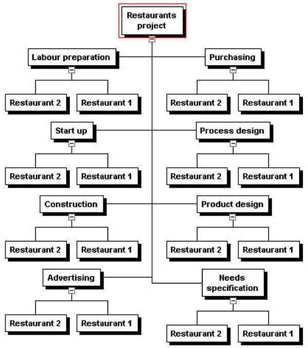
The third alternative shows a subsystem orientation.
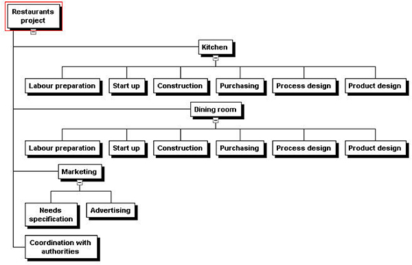
A fourth alternative shows a logistics orientation as follows:
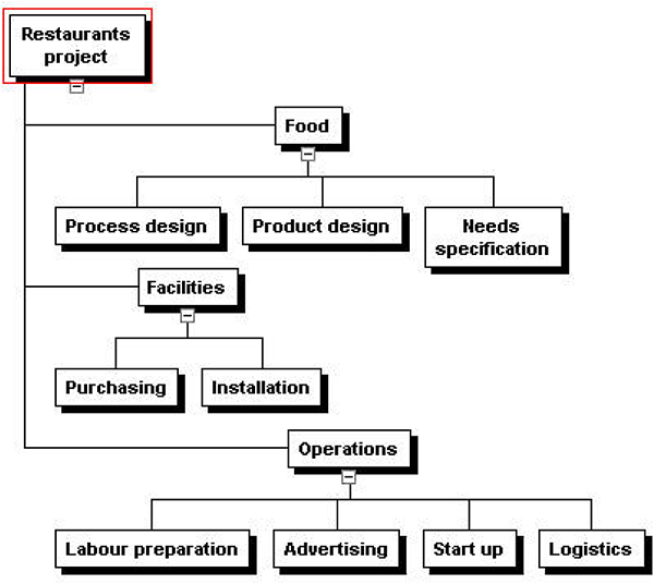
The WBS could also be drawn to show a timing orientation.

Note that ‘Design’ and ‘Execution’ are NOT work packages, they are just headings. ‘Start up’, however, is a work package since it is at the lowest level in its branch. The WBS could be broken down even further but the risk here is that the lowest-level packages could be too small. If ‘advertising’, for example, could be accomplished in 100 hours it might be a good idea to stop at that level. It could then be broken up into activities and tasks (and even sub-tasks); the duration and resource requirements would then be aggregated at the ‘advertising’ level, but not individually shown on the WBS.
It is, of course, not necessary to use a sophisticated WBS package; Excel will work just fine as the following example shows. The work packages (except ‘Start up’) are shown at level 3.

10.2 Time management
10.2.1 Exercise 2
Run ‘activity on node.xls’. Macros should be enabled; else this demo will not run.
(Use Tools->Macro->Security and adjust settings if necessary)
Start the tutorial and the following will appear.
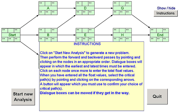
Click on ‘Start new analysis’. Note the ‘Start’ and ‘End’ nodes with zero duration.
First, the forward pass. Proceeding from left to right, click on each node and provide the ‘Earliest Start’ and ‘Earliest Finish’ times in the dialogue box. The program will alert you to any mistakes.
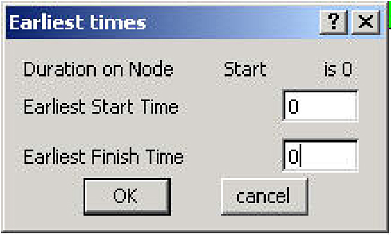
The start and finish times of the ‘start’ node is obviously 0 and 0. For all nodes with only one predecessor, the ‘Earliest Start’ time of that node equals the ‘Earliest Finish’ time of the previous node. For nodes with more than one predecessor, the ‘Earliest Start’ time obviously equals the biggest of the preceding ‘Earliest Finish’ times. The program will alert you to any mistakes.
Note that that the tasks may seem to overlap as each node starts on the same day that its predecessor finishes. This is, however, not the case. View each day as a 24-hour period starting, say, at 08h00 and finishing at 08h00 the next morning. A 1-day task could therefore start at 08h00 on Monday, day 7 of the project, and it will finish at 8h00 on Tuesday, day 8 of the project. Its successor could start at 08h00 on Tuesday, day 8.

Now the reverse pass. Start with the ‘End’ node and enter the same value as ‘Earliest Start’ and ‘Earliest Finish’ (15 in this case) for both ‘Latest Start’ and ‘Latest Finish’. For nodes with only one successor, the ‘Latest Finish’ equals the ‘Latest Start’ of its successor. In the case of multiple successors, take the smallest (earliest) value. The result looks like this:

The next step is to fill in the float, by subtracting either ‘Earliest Finish’ from ‘Latest Finish’ or ‘Earliest Start’ from ‘Earliest Finish’, i.e. top left from bottom left or top right from bottom right. Do this for all the nodes.

Finally, place the tip of the index finger (cursor) on each line that lies on the critical path (zero float) and click on the left mouse button.

The whole exercise can now be repeated. The duration of the nodes as well as their dependencies will be different for each pass.
10.2.2 Exercise 3
For this exercise we will use Plan Bee. The question might be asked why we do not use a more ‘industry standard’ software package such MS Project. The answer is very simple….the exercise is not about learning the operation of any software package…it is about mastering CONCEPTS. And so we need software that is easy to master within minutes (we do not have a lot of time!), even if it cannot handle large multimillion dollar projects.
Run Plan Bee by clicking on the desktop icon.

The following will appear.
Click file->new to start a new project.
Type in the project details and select a starting date. Click OK. Edit the first task so it reads ‘START’.

Now type in all the names of all the tasks, headings, etc. Normally you will only see around ten tasks, click on the ‘show more tasks’ button to obtain the following display. Click ‘show task options’ to return. Note that at this point all entries are tasks by default. We will change that later.

Enter the correct duration for tasks A to F.
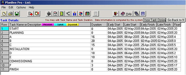
The next step is to enter the precedence relationships. Highlight each task, and then click ‘add precedence’.

In the example shown here, the precedence for A is START. Do not forget to enter the precedence for FINISH, which is F.

If you have not done this yet, select the three entries that are simply headers, not tasks, (viz, PLANNING, INSTALLATION and COMMISSIONING) and change them to ‘header level 1’ by means of the radio buttons. Notice that they are now simply headings with no duration.
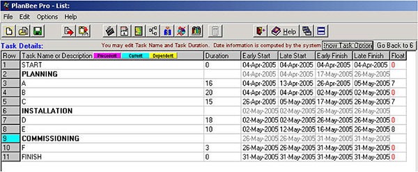
Now click on the Gantt chart icon.

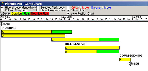
Then do the same for the PERT chart. You will need to ‘auto align Pert nodes’ and also select ‘critical this color’ to show the critical path.


10.2.3 Exercise 4
Now we have to allocate some resources. Click on the resource button.

The resource window will appear.

Now click ‘Add a new resource’ and add ‘Engineer’ with the appropriate daily rate and the number of people available. This particular screenshot shows 3 engineers but this number eventually had to be increased to 4.

Now select task A and click ‘Add Engineer to A’. Do this for all the tasks and remember to allocate 2 engineers to task C.

Then check the required resources for each day. Note that we have just enough resources for some of the days. Had we been limited to, say, 3 engineers, we would have had to delay the start date of some tasks.
Finally, click on the ‘Admin details’ button.

Once again select tasks A-F and type in the fixed cost for each task, together with cost codes and notes as applicable.
When done, click ‘file->preview/print report’ to look at a cost summary for the project.
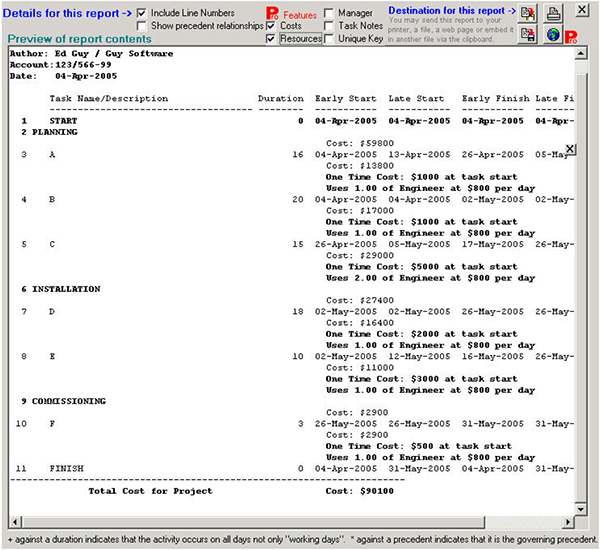
10.2.4 Exercise 5
The answer will depend on your specific example.
10.3 Cost management
10.3.1 Exercise 6
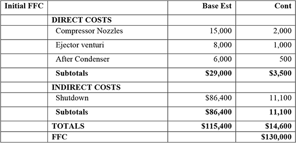

* Assumes this element of work now complete so a nil contingency is correct.
** Assumes original allowance was divided evenly across the three elements.
10.3.2 Cost Management Involving Escalation
Exercises 7, 8 and 9
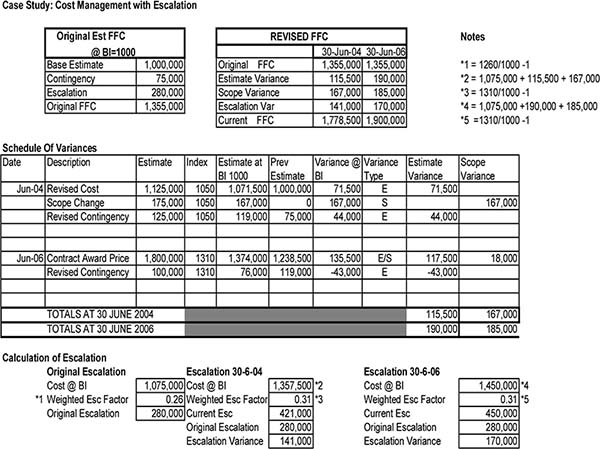
10.4 Integrated time and cost
10.4.1 Exercise 10

Exercise 11

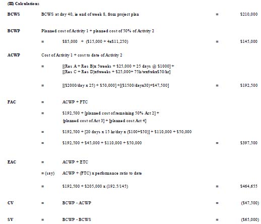
10.5 Quality management
10.5.1 Exercise 12
The answer will depend on your specific example.
10.6 Risk analysis
10.6.1 Exercise 13
The answer will depend on your specific example.
10.6.2 Exercise 14
Click Start->Run->Risk Analysis->ProjRisk

The data entry screen will appear.
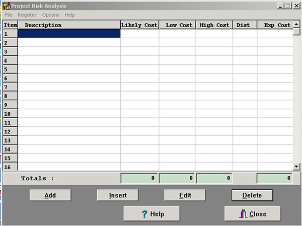
Enter the likely cost for ‘A’, as well as the maximum and minimum values, either as Dollar amounts or as percentages. Also select the type of distribution. Note that in real life the type of distribution will have to be derived from historical data.
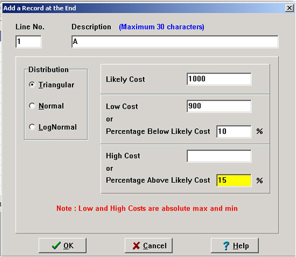
Work package ‘A’ will now appear as follows.

Enter the details for ‘B’ thru ‘F’ as well.

When done, click on the Analyze button. The software will perform a Monte Carlo simulation with 1,000 iterations (i.e. ‘rolling the dice’ 1,000 times.) The statistical distribution of the expected costs will be shown. Notice that it forms a normal distribution with a mean of $12,700 and a standard deviation of $331. It also appears highly unlikely that the cost will exceed $13,750 or that it will be less than $11,750.
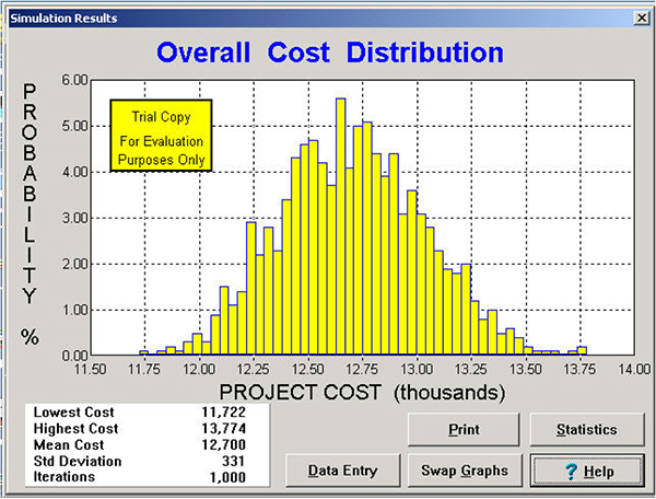
Now click ‘swap graphs’ to show the cumulative probability or ‘S’ curve. This shows the probability of the cost being less than the indicated cost.

For example, the probability of the cost being less than $13,000 is 80%. To determine the amount for 85% certainty you will need to interpolate on the graph, or select the ‘statistics’ display.

Click on the ‘Cumulative Probabilities’ tab and find the value for 85%, which is $13,049.
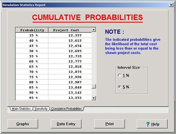
Since the original estimate was ($1,000+$1,000+$5,000+$2,000+$3,000+$500) = $12,500, it means that the contingency allocation for 85% certainty needs to be $13,049 – $12,500 = $549
10.7 Contractual issues
As in most cases of legal argument, the answer depends on a number of things which will vary from case to case. Issues arising for each situation are set out below.
10.7.1 Exercise 15
Does a contract exist? Necessary factors present include offer, acceptance, consideration, legality and capacity. A necessary factor that is absent is definite terms, i.e. “what was the bargain”?
10.7.2 Exercise 16
What is the contract? The offer (i.e. $50,000) was extinguished by the counter offer. Joe’s commencement of work is constructive acceptance of the counter offer.
10.7.3 Exercise 17
The issue is whether or not the counter offer of $8,000 remains open for acceptance until the following day. If it does, it has not been revoked.
What is reasonable in these circumstances?
10.7.4 Exercise 18
Is there a binding contract between XYZ and Mogul? Mogul’s response to XYZ is a counter offer because of the change in terms. Has the counter offer been accepted? If the postal rule of acceptance applies here, XYZ’s confirmation of May 1 is effective. Two issues may affect this rule here:
i) It could be argued that “confirm by return of post” required the communication of acceptance within a short time to be effective.
ii) Incorrect address, if the fault of XYZ, may be sufficient to overturn the rule. If the fault lay with Mogul supplying the wrong address, this is not the case.
10.7.5 Exercise 19
If the contract is binding due to a valid postal acceptance, Mogul’s letter of May 12 could be regarded as a repudiatory breach of contract. XYZ are not bound to accept the repudiation and in the circumstances are under no duty to mitigate. XYZ may be entitled to complete performance and claim the contractual sum due, which would presumably be $100,000 as the price variation clause is excluded from the contract.
This depends upon the test of “substantial interest” in proceeding with the work, rather than claiming damages.
10.7.6 Exercise 20
Fixit are in breach of contract, thus liable for damages. The test for remoteness of damages laid down in Hadley v Baxendale applies, i.e. was the loss of profit from losing the armed forces contract within Fixit’s knowledge.
There is a duty on Millicent to mitigate her losses. An important issue will be whether or not it was reasonable for her to reject Fixit’s offer to install a temporary system.
10.7.7 Exercise 21
The fact that the provision is referred to as ‘agreed damages’ will not prevent the Court finding it to be a penalty if that is its true nature.
In this case damages claimed are $80,000. Applying the formula for 8 weeks’ delay gives $110,000 under this provision. Likely to be considered a penalty, and thus non-recoverable.
The $10,000 by itself appears to be a penalty. It arises if Fixit is half a day late or 20 days late, and therefore does not appear to be an assessment of losses in the normal course of the business.
10.8 Project quality plan
Exercise 22 A recommended format for your Project Quality Plan outline is set out below. Specific requirements may vary for different projects.
PROJECT QUALITY PLAN OUTLINE
PQP SIGN OFF
PROJECT OBJECTIVES
(Include defined Project Success Criteria)
PROJECT CHARTER
MANAGEMENT AUTHORISATION
DELEGATED AUTHORITIES
PROJECT PLAN
SCOPE DEFINITION
WORK BREAKDOWN STRUCTRE
ORGANISATION STRUCTURE
RESPONSIBILITY MATRIX (optional – depending on complexity)
SCHEDULE
BUDGET
PROJECT CONTROLS
SYSTEM OUTLINES
PROJECT ADMINISTRATION
Filing systems
Document management
Correspondence management
Meetings
REPORTING
Specific Client requirements: e.g., specifically address Project Success Criteria by defining relevant, measurable, project performance indicators.
RISK MANAGEMENT STRATEGIES
DESIGN MANAGEMENT
Quality Policies
Standards
Tendering strategies
Value Management strategies
PROCUREMENT MANAGEMENT (SUPPLY & INSTALLATION)
Procurement strategies
Quality policies
Standards
Tendering strategies
PROCEDURES
(This example is for a typical capital works project)
PROJECT ADMINISTRATION
Document management
Correspondence management
Meetings
REPORTING
Procedures & formats
SCOPE MANAGEMENT
Briefing
Change control
QUALITY MANAGEMENT
Design ITPs
Design quality verification
Construction ITPs
Construction quality verification
TIME MANAGEMENT
Schedule preparation
Schedule revisions
Monitoring & reporting
COST MANAGEMENT
Estimating
Budgeting
Financial authority
Monitoring & reporting
RISK MANAGEMENT
Risk management processes
CONTRACT MANAGEMENT
Tender & contract documentation
Tendering & tender evaluation
Variation procedures
Contract administration
Budgets, Variance Analysis, Cost Reporting and Value Management
A1 Budget presentation
A1.1 Introduction
For effective running of a business, management must know:
- Where it intends to go (organizational objective)
- How it intends to accomplish its objective (plans)
- Whether individual plans fit in the overall organizational objective (coordination)
- Whether operations conform to the plan of operations relating to that period (control).
Budgetary control is the device that an organization uses for all these purposes.
A1.2 Budget
A budget is a quantitative expression of a plan of action relating to the forthcoming budget period. It represents a written operational plan of management for the budgeted period. It is always expressed in terms of money and quantity. It is the policy to be followed during the specified period for attainment of specified organizational objectives.
In CIMA terminology, a budget is defined as follows:”A plan expressed in money. It is prepared and approved prior to the budget period and may show income, expenditure, and the capital to be employed. May be drawn up showing incremental effects on former budgeted or actual figures, or be compiled by zero-based budgeting.”
A1.3 Budgetary control and budgeting
The terms budgetary control and budgeting are often used interchangeably to refer to a system of managerial control. Budgetary control implies the use of a comprehensive system of budgeting to aid management in carrying out its functions such as planning, coordination and control.
In CIMA terminology: “Budgetary control is the establishment of budgets relating to responsibilities of executives to the requirement of a policy, and the continuous comparison of actual with budgeted results either to secure by individual action the objective of that policy or to provide a basis for revision.”
A1.4 Budgets and forecasts
A forecast is a prediction of what is going to happen as a result of a given set of circumstances. A forecast is a mere assessment of future events and the budget is a plan of action proposed to be adhered to during a specified period. Budgets start with forecasting and lead to a control process, which continues even after budget preparation. A forecast includes projection of variables either controllable or non-controllable that are used in development of budgets.
A1.4.1 Fixed budget
A fixed budget is a budget that is used unaltered during the budget period. It is prepared for a particular activity level and it does not change with actual activity level being higher or lower than the budgeted activity level. This budget does not highlight the ‘activity variance’, and the absolute differences of budgeted figures and actual figures will be calculated without any type of adjustment. It may roughly meet the needs of profit planning, but it is almost completely inadequate as a cost control technique as there is no criterion to immediately highlight good or bad performance.
A1.4.2 Flexible budget
A flexible budget is a budget which, by recognizing different cost behavior patterns, is designed to change as volume of output changes. It is also known as a variable budget. The main characteristic of a flexible budget is that it shows the expenditure appropriate to various levels of output. If the volume changes, the expenditure associated with it can be established from the flexible budget for comparison with actual expenditure as a means of control. It provides a logical comparison of budget allowances with actual cost, i.e., a comparison with a like basis. Flexible budgeting helps both in profit planning and operating cost control. In-depth cost analysis and cost identification is required for preparation of this budget, which will involve categorizing the expenses as fixed, variable and semi-variable. Fixed items of expenditure will remain same for all level of activity. For items of variable expenditure, rate per unit of activity is determined and based on this relationship, variable expenses for any level of activity is determined. Extra efforts are made in analyzing semi-variable items of expenditure in fixed and variable elements. A flexible budget constitutes a series of fixed budgets, i.e., one fixed budget for each level of activity.
A1.5 Establishment of functional budgets and a master budget
A1.5.1 Sales budget
The sales budget is the most important functional budget and it primarily forecasts what the organization can reasonably expect to sell both in quantity and value during the budget period. A sales budget can be prepared showing sales under any one or combination of the headings: Product, Territory, Types of customers, Salespersons, Period (month, quarter or week).
Illustration -1:
AARK Associates manufactures three products X, Y and Z and sell them through three divisions, North, South and West. Sales budgets for the current year based on the estimates of Division Managers (Sales), were:

Actual sales for the current year were:


Sales prices are $12, $8 and $10 in all areas. It was found by the market research team that Product X finds favor with customers, but is under-priced. It is expected that if the price is increased by $1.00, its sales will not be affected. The price of product Y is to be reduced by $1.00 as it is overpriced. Product Z is properly priced, but extensive advertisement is required to increase its sales.
On the basis of the above information, the Divisional managers estimate that the increase in sales over the current budget will be
It is also expected that there will be a further rise in sales thanks to extensive advertising and the figures could be

We have to prepare a sales budget along with budgeted and actual sales for the current year.
AARK Associates
Presented By –
Checked By –
Submitted on –


A1.5.2 Production budget
This shows the quantities to be produced for achieving sales targets and for keeping sufficient inventory. Budgeted production is equal to projected sales plus closing inventory of finished goods minus opening stock of finished goods. It is a forecast of production for budgeted period and is prepared in physical units. It is necessary to coordinate the Production Budget with the Sales Budget to avoid imbalance in production. It is an important budget and forms the basis for preparation of material, labor and factory overhead budgets.
Illustration -2:
The SPG & Co. plans to sell 108,000 units of a certain product line in the first quarter, 120,000 units in the second quarter, 132,000 units in the third quarter, 156,000 units in the fourth quarter and 138,000 units in the first quarter of the following year. At the beginning of the first quarter of the current year, there are 18,000 units in stock. At the end of each quarter the company plans to have an inventory equal to one-sixth of the sale for the next quarter. We have to calculate the number of units that must be manufactured in each quarter of the current year.
Solution:

A1.5.3 Production cost budget
Production cost budget expresses the cost of carrying out production plans and programs set out in the production budget. It summarizes the material budget, labor budget and factory overhead budget for production.
A1.5.4 Material budget
It shows the estimated quantity as well as the cost of each type of direct material required for producing the number of units listed in the production budget. It serves the following purposes:
- It forms the basis for the purchase cost budget
- It helps the purchase department plan purchase to avoid default in delivery of material
- It forms the basis for the determination of the minimum and the maximum levels of inventory of material and components
A1.5.5 Purchase budget
This budget sets out the ‘purchase’ plan of the company during the budget period. It is prepared considering factors like storage capacity and finance available so that capital tied up in stock is minimized while the production program continues smoothly.
Illustration -3:
VSAX Limited manufactures three products: A, B and C. It is required to prepare budgets for the month of January, 2004 for:
- Sales in quantity and value, including total value
- Production quantities
- Material usage in quantities
- Material purchases in quantity and value, including total value
Data available is tabulated below

Materials used in the company’s products are:

Solution:
1. Sales Quantity and Value Budget
2. Production Quantities Budget

3. Material Usage Budget (Quantities)

4. Material Purchases Budget (quantities and values)

A1.5.6 Labor budget
This contains the estimates relating to the number and type of employees required for the budgeted output. Labor required is classified according to grades and thereafter the estimated rate per hour and hence the labor cost per unit is arrived at.
A1.5.7 Overhead budget
Companies divide their overhead costs in two categories for the purpose of control – fixed overhead and variable overhead. Depreciation, insurance and taxes are the main items that fall within the fixed overhead category. Variable overheads include indirect material, indirect labor and indirect expenses, which are used according to production.
Illustration -4:
The following data is available in a manufacturing company for a yearly period:
| Fixed Expenses: | $ Millions |
|---|---|
| Wages and salaries | 9.5 |
| Rent, rates and taxes | 6.6 |
| Depreciation | 7.4 |
| Sundry administration expenses | 6.5 |
| Semi-variable Expenses (At 50% of activity) | |
| Maintenance and repairs | 3.5 |
| Indirect labor | 7.9 |
| Sales department salaries, etc. | 3.8 |
| Sundry administration expenses | 2.8 |
| Variable expenses (At 50% of activity) | |
| Material | 21.7 |
| Labor | 20.4 |
| Other expenses | 7.90 |
| Total Cost | 98.0 |
The fixed expenses remain constant for all levels of production; semi-variable expenses remain constant between 45% and 60% of capacity, increase by 10% between 65–80% and by 20% between 80–100% capacity.
| Sales at various levels are: | $ Millions |
| 50% Capacity | 100 |
| 60% Capacity | 120 |
| 75% Capacity | 150 |
| 90% Capacity | 180 |
| 100% Capacity | 200 |
We have to prepare a flexible budget for the year and forecast the profit at 60%, 75%, 90% and 100% of capacity.
Solution:
Flexible Budget for the period


A1.5.8 Research and development budget
Research activities include the development of new products, betterment of existing products and improvement of processes. The expenditure of research depends on the nature of the company’s products, economic conditions, competition, technological developments in the related industry and the policy of management. Research expenditure is often based on an established percentage of sales or estimated amounts expected to be available during the forthcoming budget period.
A1.5.9 Capital expenditure budget
It represents the expected expenditure on fixed assets during the budget period. Capital expenditure budget relates to projects involving huge capital outlay and long-term commitment. Most of the capital investment decisions affect operations of business over a series of years and large risks and uncertainties are associated with these decisions.
A1.5.10 Cash budget
It is a forecast of cash flows, i.e. receipts during the budget period. Preparation of cash budget is based primarily on following information:
- Detailed estimate of cash receipts
- Detailed estimate of cash disbursement
- Time-lag induced by credit transactions
- Time-lag in terms of revenue and expenditure
Cash budgets are not made for performance evaluation. It ensures company’s liquid position sound to meet its daily requirement. Cash budget is prepared by any of the following methods:
- Receipt and payment method – Under this method, all receipts and payments which are expected during the period should be considered. Accruals and adjustments are excluded while preparing the cash budget by receipt and payment method. All anticipated cash receipts are added to the opening balance of cash. The expected cash payments are deducted from this to arrive at the closing balance of cash for the month.
- Adjusted profit and loss account method – This method is based on the assumption that profit is equivalent to cash. The adjustments made to arrive at the profit will be added back, if these adjustments do not involve cash outflow. For example, depreciation on fixed assets, accrued expenses, etc., will be added back to profit to arrive at the cash balance available at the closing date. It is used for making long-term cash forecast.
- Balance sheet method – In this method, a forecast balance sheet is prepared considering changes in all items (except cash) of balance sheet like fixed assets, plant and machinery, furniture and fixtures, debtors, share capital, debentures and creditors, etc. The two sides of balance sheet are balanced and the balancing figure represents closing balance of cash.
A1.5.11 Plant utilization budget
This budget sets out the plant and machinery requirements to meet the budgeted production during the budget period. The plant capacity is expressed in terms of convenient units such as working hours, weight or number of units, etc. It highlights the budgeted machine load in each department and focuses attention on overloading so that remedial action can be taken in time to explore the alternatives like shift working, purchase of new machinery, working overtime and sub-contracting, etc. It also highlights under loading and seeks increase in sales volume by reduction in prices, discounts, change in terms of payment and advertising, etc.
A1.5.12 Master budget
After all the functional budgets have been prepared, these are summarized in the form of a summery budget which gives a forecast profit and loss account and forecast balance sheet for the budget period. The summery budget (after necessary correction) is presented to the Board of Directors for approval and after approval the same is called the Master Budget. It is the organization’s formal plan of action for the forthcoming budget period and is an integrated form of all functional budgets bearing approval of top management. In the master budget, costs are classified and summarized by types of expenses as well as by departments. The advantages of a Master Budget are as follows,
- It is an approved document which shows projected profit position of the organization
- Preparation of master budget enforces coordination among functional budgets
- Budgeted balance sheet shows the projected financial position of the organization
Functional budgets represent sectional goals for the budget period. Preparation of master budget basically starts from the previous year’s profit and loss account, balance sheet and set of information and instructions for the forthcoming budget period.
A1.6 Zero-base budgeting
Zero-base budgeting is a new technique of planning and decision making and reverses the working process of traditional budgeting. The concept of zero base budgeting has gained world-wide eminence after Peter Pyhr of Texas Instruments Inc. used it. Traditional budgeting starts with the previous year’s expenditure level as a base and then discussion is focused to determine the ‘cuts’ and ‘additions’ to be made. In zero-base budgeting no reference is made to previous levels of expenditure. A convincing case is made for each decision unit to justify the budget allotment for the unit during that period and each decision unit is subjected to thorough analysis to determine the relative priorities between different items included in it. Zero base budgeting is completely indifferent to whether the total budget is increasing or decreasing. It identifies the alternatives so that if more money is required in one department, it can be saved in another area. CIMA has defined it ‘as a method of budgeting whereby all activities are re-evaluated each time a budget is set. Discrete levels of each activity are valued and a combination chosen to match funds available.’ (see Figure A1.1)

System concepts relating to traditional and zero-based budgeting
A1.6.1 Advantages
It is a healthy process that promotes self-searching among the managers and is used with the object of finding out most useful alternatives for available resources of a company. Main advantages are as follows:
- All proposals, old and new, compete equally for scarce resources
- It drives managers to find out cost effective ways to improve operations
- It requires less paper work than traditional budgeting because the proposal goes from bottom all the way to top. It avoids successive appraisals at various levels of management
- It detects deliberately inflated budget request
- It identifies complete impact of spending money on a particular project
Steps involved in the introduction of zero-base budgeting
- Corporate objectives should be established and laid down in detail.
- Decision units should be identified by dividing the organization according to functions, operations or activities for detailed analysis.
- An analysis and documentation of each decision unit should be done by a responsible manager keeping the following points in view:
- Current operations of decision units should be identified and linked with organizational objectives
- Alternatives to meet the target should be expressed
- Best alternative should be selected and effects that are required to accomplish the alternative should be documented
- ‘Decision units’ should be split into decision packages ranked in order of priority.
- Budget staff will compile operating expenses for packages approved by departmental heads.
Zero base budgeting is primarily based on development of decision units, identification of decision packages and ranking of decision packages.
Decision units
An organization is divided into decision units. Managers of decision units justify the relative budget proposal. Any base may be adopted for dividing the organization into decision units; products, markets, customer groups, geographical territories, capital projects. The division of organization among its decision units should be logically linked with organizational objectives.
Identification of ‘decision packages’
Each manager should break down his decision unit into smaller decision packages. A decision package has been defined as a document that distinctly identifies a function, operation or an activity. A decision package will be evolved with reference to particular circumstances and should have the following elements:
- Identification of data
- Economic benefits
- Alternative course of action
- Intangible benefits
Ranking decision packages
By ranking decision packages, a company is able to weed out a lot of marginal efforts. Scarce resources of an organization should be directed at the most promising lines only. The ranking process is used to establish a rank priority of decision packages within the organization. During the ranking process managers and their staff will analyze each of the several decision package alternatives. The analysis allows the manager to select the one alternative that has the greatest potential for achieving the objective(s) of the decision package. Ranking is a way of evaluating all decision packages in relation to each other. Since, there are any number of ways to rank decision packages managers will no doubt employ different methods. The main point is that the ranking of decision packages is an important process of Zero-Base Budgeting. A decision package is ranked keeping the following points in view.
- Necessity of introducing programs
- Technical competence of the company in attempting the programs
- Economic benefit analysis relating to the programs
- Operational feasibility of introducing programs.
- Study of risk involved in abandoning the programs
A1.6.2 Disadvantages of Zero-Based Budgeting
- Difficult to define decision units and decision packages, as it is very time-consuming and exhaustive.
- Forced to justify every detail related to expenditure. The R&D department is threatened whereas the production department benefits.
- Necessary to train managers. Zero-base budgeting should be clearly understood by managers at various levels otherwise they cannot be successfully implemented. Difficult to administer and communicate the budgeting because more managers are involved in the process.
A1.7 Program budgeting
Program Budgeting was introduced in the U.S. Department of Defense in 1961. Its utilization became extremely common by 1968, in federal as well as local government of the United States of America. Conventional budgeting works well in profit oriented organizations. Program budgeting came into existence for Government Departments and non-profit institutions. In program budgeting emphasis is laid on formulation of different budgets for different programs. It integrates all of the organization’s planning activities and budgeting into a total system. First programs for the mission of the organization are identified. Then each program is broken into elements, or each element’s resources i.e., material, manpower, facilities and capital are identified. Allocation of resources to various programs is taken into account. Great stress is continuously placed on analysis of alternatives and estimating cost of accomplishing objectives and fulfilling purposes and needs. The program budgeting format is illustrated here in Figure A1.2.

Format illustrating the idea of program budgeting
First resources over the period are identified for different elements and then the cost of these elements is aggregated to arrive at the cost of a program. For appraising public projects program budgeting uses micro-economies. The flow chart in Figure A1.3 illustrates the difference between the traditional budget format and the program budget format.

Difference between traditional and program budget format
Program budgeting includes:-
- Identification of programs required to fulfill the mission
- Identification of program elements
- Allocating resources to programs
- Utilizing forecast studies analysis
Quantification of data in considerable detail is necessary because budgeting consequences of approved programs are anticipated and actual performance is compared with budget performance of programs. In non-profit organizations it is necessary to identify the output indicators because output cannot be measured in terms of money e.g., for an on-the-training program, output indicator may contain number of workers trained. Similarly for health program, output indicator may lower disease incidence. Program budget does not eliminate the need for traditional budget and very useful for multi-year forecasts. It adds new dimension to planning analysis and budgeting. Traditional budgeting emphasizes the method and means used, program budgeting emphasizes the purposes and the objectives of the program.
A1.8 Performance budget
The ‘Performance Budget’ was originally used in the United States by the First Hoover Commission in 1949, when it recommended the adoption of a budget based upon functions, programs and activities. It emphasizes work-cost measurement and managerial efficiency. Cost and production goals are established and then compared to actual performance. It provides output-oriented information with a long range perspective to allocate resources more effectively.
A performance budget is one which:
- Presents the purposes and objects for which funds are requested
- The costs of activities proposed for achieving these objectives
- Quantitative data measuring the accomplishments
- Work performance under each activity.
In program budgeting, the principal emphasis is on programs, identification of their elements and determination of cost for each program. In performance budgeting stress is on activities approved by the company and determination of cost of each activity.
A1.8.1 Performance Budgeting vs Program Budgeting
- Performance is based on the past and prior accomplishment whereas program is essentially a forward looking approach. Programmed budgeting is useful for review and decision making at and above the departmental level.
- Performance budget has drawn inspiration from cost accounting and scientific management. Program budgeting has drawn its core of ideas from economics and systems analysis.
- In the performance budgeting literature, budgeting is described as a tool of management and the budget as a work program where as under program budgeting, budgeting is an allocation process among competitive claims and the budget is a statement of policy.
A1.8.2 Performance budgeting vs Traditional Budgeting
- Decision making is primarily downward in performance budgeting. In traditional budgeting the flow of budgetary decisions is primarily upward.
- Performance budgeting requires that budgetary decisions be made by emphasizing output categories such as goals, purposes, objectives and products or services, instead of salaries, materials and facilities as in the case of traditional budgeting.
- Performance budgeting focuses on future impacts of current major decisions whereas traditional budgeting is retrospective, i.e., measuring what was done with current means in estimating the next budget year.
A1.8.3 Stages of Performance Budgeting
Objectives
The objective of individual activities is clearly spelt out in quantitative and monetary terms as far as possible. These objectives are matched against the long term objectives of Government.
Analysis
The long-term strategy and short-term tactics for achieving the desired objectives are considered. In addition, possible alternative activities are identified and costs and their benefits are worked out. After detailed analysis, the activities are selected.
Classification
The activities taken for implementation are classified with reference to a prescribed classification system. This approach facilitates allocation of resources to selected activities.
Organization
The role of different implementing agencies in achieving the specified objectives are clearly demarcated and financial rules and accounting system are modified to implement the defined activities more effectively.
Evaluation
A proper system for evaluating the implementing of activities is predetermined. Desired information system and reporting system relating to financial, physical and economic data are also installed to monitor the desired activities during execution. The projects should be subject to thorough evaluation even after their completion (see Figure A1.4).

Five stages of performance budgeting
The five stages of performance budgeting are shown in Figure A1.4 where the clockwise arrows represent the activity flow of the system, while the anticlockwise broken arrows represent the feedback process. The tangential arrows represent the interface with the outside world.
A1.9 Participative budgeting
It is a commonly observed that lack of involvement in formulation of goals and objectives always leads to restricted efforts and output which is fatal for improvement of productivity. Optimum output requires greater participation of operating managers in budgeting process. Participative budgeting is the practice of allowing all individuals who are responsible for performance under a budget. It is the budgeting approach, which ensures that all concerned staff members and maximum coordination.
The advantages are summarized below:
- It provides operating manager with a sort of challenge for implementation of the budget
- Operating managers feel a sense of responsibility to implement the budget, when they have been a party to the decisions
- Operating staff consider the budget as their own goal and sense of achievement in completion
A1.10 Responsibility accounting
Responsibility accounting emphasizes the division of an organization among different sub-units in such a way that each sub-unit is the responsibility of an individual manager. The basis of this approach is that a manager should be held responsible for those activities, which are under his or her direct control. It recognizes cause and effect relationship between a Manager’s decisions and actions and its impact on cost and revenue results.
A1.10.1 Pre-requisites for responsibility accounting
- The area of responsibility and authority of each center should be well defined (organizational chart)
- There should be a clear set of goals for the manager of each responsibility center
- The performance report of each center should contain only revenues, expenses, profits and investments that are controllable by the manager of that responsibility center
- Performance reports for each responsibility center should be prepared highlighting variances
- The manager of each responsibility center should participate in establishing the goals that are going to be used to measure their performance
A1.10.2 Responsibility centers
There are five types of responsibility centers for the management control purpose and each center can be defined as a unit of function of an organization headed by a manager having direct responsibility for its performance.
Cost center
Responsibility in a cost center is restricted to cost alone. Cost center is a segment of the firm that provides tangible or intangible service to departments. In manufacturing environments, all production centers and service centers are termed as separate cost centers. CIMA defines ‘cost center’ as a production or service location, function, activity or item of equipment whose costs may be attributed to cost units.
Revenue center
The revenue center is the smallest segment of activity or an area of responsibility for which only revenues are accumulated. A revenue center is a part of that organization whose manager has the primary responsibility of generating sales revenues but has no control over the investment in assets or the cost of manufacturing a product. CIMA defines revenue center as a center devoted to raising revenue with no responsibility for production.
Profit center
CIMA defines profit center as a part business accountable for costs and revenues. It may be called a Business Center, Business Unit (BU), or Strategic Business Unit (SBU). A profit center is a segment of activity for which both revenues and costs are accumulated. Generally, most responsibility centers are viewed as profit centers, taking the difference between revenues and expenses.
Investment center
CIMA defines investment center as a profit center whose performance is measured by its return on capital employed. Investment center is a segment of activity for areas held responsible for both profits and investment. For planning purposes, the budget estimate is a measure of rate-of-return on investment and for control purposes, the performance evaluation is guided by a return on investment variance.
Contribution center
Contribution center is an area of responsibility for which both revenues and variable costs are accumulated. CIMA defines contribution center as a profit center whose expenditure is reported on a marginal or direct cost basis. The main objective of a contribution center manager is to maximize the center’s contribution
Illustration -5:
In a cotton textile mill, the spinning superintendent, weaving superintendent and the processing superintendent report to the Mill Manager who along with the Chief Engineer reports to Director (Technical).The sales manager along with publicity manager reports to the Director (Marketing) who along with the Director (Technical) reports to the Managing Director.
The following monetary transactions ($) have been extracted from the books for a particular period.
A = Adverse; F = Favorable

We have to prepare responsibility accounting reports for the Managing Director, Director (Marketing), Director (Technical) and Mill Manager.
Solution:
Responsibility Accounting Reports
| Budget | Actual | Variance | |
| 1. For Mill Manager | |||
| A. Spinning Superintendent | |||
| Raw Materials | 2,800,000 | 2,920,000 | 120,000(A) |
| Labor | 800,000 | 840,000 | 40,000(A) |
| Utilities | 150,000 | 165,000 | 15,000(A) |
| Total A | 3,750,000 | 3,925,000 | 175,000(A) |
| B. Weaving Superintendent | |||
| Materials | 100,000 | 105,000 | 5,000(A) |
| Labor | 600,000 | 620,000 | 20,000(A) |
| Utilities | 200,000 | 190,000 | 10,000(A) |
| Total B | 900,000 | 915,000 | 15,000(A) |
| C. Processing Superintendent | |||
| Raw Materials | 7,00,000 | 6,40,000 | 60,000(F) |
| Labor | 500,000 | 512,000 | 12,000(A) |
| Utilities | 300,000 | 350,000 | 50,000(A) |
| Total C | 1,500,000 | 1,502,000 | 2,000(A) |
| D. Mill Manager’s Salaries & Admin. | 100,000 | 105,000 | 5,000(A) |
| Total of Mill Manager (A+B+C+D) | 6,250,000 | 6,447,000 | 197,000(A) |
| 2. For Chief Engineer | |||
| Maintenance Stores | 200,000 | 190,000 | 10,000(F) |
| Maintenance Labor | 260,000 | 255,000 | 5,000(F) |
| Maintenance Utilities | 50,000 | 60,000 | 10,000(A) |
| Total for Chief Engineer | 510,000 | 505,000 | 5,000(F) |
| 3. For Director Technical | |||
| Mill Manager | 6,250,000 | 6,447,000 | 197,000(A) |
| Chief Engineer | 510,000 | 505,000 | 5,000(F) |
| Office Salary and Admn. | 175,000 | 200,000 | 25,000(A) |
| Total for Director Technical | 6,935,000 | 7,152,000 | 217,000(A) |
| 4. For Director Marketing | |||
| A. Sales Manager | |||
| Income – Sales | 10,000,000 | 8,800,000 | 1,200,000(A) |
| Expenditure – Traveling | 40,000 | 42,000 | 2,000(A) |
| Sales Commission | 2,50,000 | 240,000 | 10,000(F) |
| Salary and Admn. | 100,000 | 95,000 | 5,000(F) |
| Total A | 3,90,000 | 3,77,000 | 13,000(F) |
| B. Publicity Manager | |||
| Salary and Admn. | 120,000 | 130,000 | 10,000(A) |
| Publicity Expenditure | 200,000 | 198,000 | 2,000(F) |
| Total B | 320,000 | 328,000 | 8,000(A) |
| C. Director Marketing | |||
| Sales manager Expenditure | 390,000 | 377,000 | 13,000(F) |
| Publicity manager | 320,000 | 328,000 | 8,000(A) |
| Salary and Admn. | 200,000 | 190,000 | 10,000(F) |
| Total Expenses | 910,000 | 895,000 | 15,000(F) |
| 5. For Managing Director | |||
| Mg. Dir.’s office staff | 250,000 | 270,000 | 20,000(A) |
| Director Marketing | 910,000 | 895,000 | 15,000(F) |
| Director Technical | 6,935,000 | 7,152,000 | 217,000(A) |
| Total Expenses | 80,95,000 | 83,17,000 | 222,000(A) |
| Sales Manager (Income) | 10,000,000 | 8,800,000 | 1,200,000(A) |
| Profit | 1,905,000 | 483,000 | 1,422,000(A) |
Case Study – A
I. Product X is produced from two materials: C and D. Data in respect of these materials is as follows:
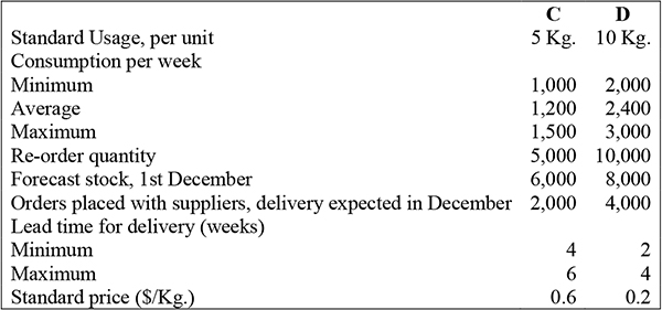
During January there is to be an intensive sales campaign and to meet the expected demand, the production director requires the stocks of materials and product X to be at maximum level at 31st December.
Data in respect of product X are as follows:

A) From the above data you are required to prepare for the month of December:
- Production budget
- Purchase budget
B) Calculate the optimal re-order quantities in respect of material C based on data given above and that:
- A 50 week – year is in operation.
- The cost of placing each order is Rs.5.
- The cost of storage is 25% per annum of the value of the stock held.
Hint:
- Maximum level = Re-order level/ (Re-order quantity – minimum consumption during the period required to obtain delivery).
- Re-order level = maximum usage × maximum re-order period.
- Minimum level = minimum usage × minimum lead time.

II. A company manufacturing two products using only one grade of direct labor is shown below from next year’s budget.

The stock of finished goods at the beginning of the first quarter is expected to be 3,000 units of product M and 1,000 units of product N. Stocks of work in progress are not carried.
Inspection is the final operation for product M and it is budgeted that 20% of production will be scrapped. Product N is not inspected and no rejects occur.
The company employs 210 direct operators working a basic 40-hour week for 12 weeks in each quarter and the maximum overtime permitted is 12 hours per week for each operator.
The standard direct labor hour content of product M is 5 hours per unit and for product N, 3 hours per unit. The budgeted productivity (efficiency) ratio for the direct operatives is 90%.It is assumed both M and N are profitable.
Calculate the budgeted direct labor hours required in each quarter of next year and to which the direct labor available can meet these budgeted requirements. Also suggest alternative action to minimize the shortfall or surplus of labor hours to achieve each quarter’s sales budget.
A2 Variance Analysis
A2.1 Introduction
The comparison of actual performance with standard performance reveals the variances. A variance represents a deviation of the actual results from the standard results. There can be cost variances, profit variances, sales value and operational and planning variances.
Variance analysis is an exercise that tries to isolate the causes of variances in order to report to management those situations which can be corrected and controlled by timely action. Variance analysis is used for decision making e.g., an unfavorable price variance for raw materials may lead to looking for an alternative supplier and/or to increase the price of the product. It is also used for incentives/control. In accordance with the principal of controllability those factors a manager can control by means of variances are isolate.
Variance analysis should be a continuous process for the following reasons:
- Labor rates, salary levels etc., change due to union negotiations, policy decisions or changes in composition of the work force
- Selling price changes
- In a multi-product company, product mix changes and different lines have different margins; the overall profit position will change
- Improvement in systems can bring about reduction in costs
- Change in level of efforts of operators, supervisors etc. can affect existing cost levels
- Investment in new capital equipment and scrapping of old equipment/processes/methods can affect the operating cost levels
- The prices of bought-out material may vary
- Changes in product design may change cost-inputs
- Changes in organizational structure may affect cost levels
- The amount of idle time may change due to holdups, strikes, lockouts and power failure.
A2.2 Model steps
The ‘model steps’ approach has been adopted in computing variances. These model steps have been arranged in a logical sequence which should be necessarily adhered to for arriving at the correct inferences. Variance analysis is to measure performance, correct inefficiencies, and deal with accountability.
Variances can be favorable or adverse (unfavorable).
These are illustrated in Figure A2.1

Variances
Favorable variance = the actual amount < the standard amount. Favorable variances are credits; they reduce production costs.
Adverse variance = the actual amount > the standard. Adverse/Unfavorable variances are debits; they increase production costs. This works for each individual cost variance and when a total variance is computed.
A favorable variance does not necessarily mean it is desirable, nor does an unfavorable variance mean it is not desirable.
It is for the management to analyze all variances to determine the cause in the following manner
- Determine if standard is correct
- Consider costs vs benefits in reviewing standards
Whether a variance is favorable or unfavorable is ultimately determined with reference to its impact on profit. Each model step represents the existence of a particular variance. If the value of the step is zero then the value of the step immediately preceding the analyzed step should be considered for calculating variance.
A2.3 Cost variance
Cost Variance represents the difference between the costs actually incurred for production and the costs specified for the same. It is the sum total of following variances:
- Direct material cost variance
- Direct wage variance
- Variable overhead variance
- Fixed overhead variance
A2.3.1 Direct material cost variance
Direct material cost variance and its sub-divisions are illustrated in Figure A2.2
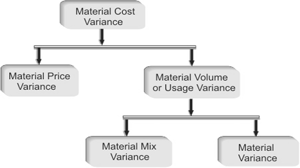
Direct material cost variance
Model steps
Four model steps are given here for calculating the material cost variances
- M1 – Actual cost of material used = Actual quantity of material used × Actual rate.
- M2 – Standard cost of material used = Actual quantity of material used × Standard rate.
- M3 – Standard cost of material used if it had been used in the standard proportion.
- M4-Standard material cost output = Standard quantity of material required for the specified output × Standard rate.
Material cost variance
It is the difference between actual cost of material used and standard cost of material specified for output achieved. Material cost variance arises due to variation in price and usage of materials. Difference between M1 and M4 will be the material cost variance.
Material price variance
Material price variance is the difference between the actual price paid and standard price specified for the material. It represents the difference between the standard cost of actual quantity purchased and actual cost of these materials. Difference between M1 and M2 will be the material price variance. The material price variance is uncontrollable and provides management with information for planning and decision making purposes. It helps the management increase product price, use substitute materials or find other (offsetting) sources of cost reduction.
Material usage or volume variance
It indicates whether or not material was properly utilized and is also referred to as quantity variance. Material usage or volume variance is the difference between actual quantity used and standard quantity specified for output. A debit balance of material usage (variance) indicates that material used was in excess of standard requirements and credit balance indicates saving in the use of material. Difference between M2 and M4 will be material usage or volume variance.
Material usage variance consists of material mix variance and material yield variance. The favorable material usage variance is not always advantageous to the company as it may be related to an unfavorable labor efficiency variance, e.g. labor may have conserved material by operating more carefully at a lower output rate.
Material mix variance
It is the difference between the actual composition of the mix and the standard composition of mixing the different types of materials. Short supply of a particular material is often the common reason for material mix variance and it is the difference between M2 and M3.
Material yield variance
In certain cases, it is observed that output will be a particular percentage of total input of material e.g., 80% of the total input of material will be the expected output. If the actual yield obtained is different from that of the standard yield specified, there will be yield variance. Difference between M3 and M4 will be the material yield variance.
Illustration –6:
The standard cost of a certain chemical mixture is as under:
- 40% of material A at $20 per kg
- 60% of material B at $30 per kg
A standard loss of 10% is expected in production. The following actual cost data is given for the period.
- 180 kgs material A at a cost of $18 per kg
- 220 kgs material B at a cost of $34 per kg
The weight produced is 364 kgs.
We have to calculate the following:
- Material price variance
- Material mix variance
- Material yield variance
- Material cost variance
- Material usage variance
Solution:
M1 – Actual cost of Material used:
Material A – 180 kgs × $18 = $3240
Material B – 220 kgs × $34 = $7480
M1= $10,720
M2 – Standard cost of Material used:
Material A – 180 kgs × $ 20 = $3600
Material B – 220 kgs × $ 30 = $6600
M2= $10,200
M3 – Standard cost of Material, if it had been in standard proportions.
Standard mix in kgs
Material A = (Weight in actual mix × standard rate of material A per kg × standard mix in kg)/ weight of standard mix = 400 kgs × $20 × 40 kgs/100 kgs = $3,200
Material B = (Weight in actual mix × standard Rate of material A per kg × standard mix in kg)/ weight of standard. mix = 400 kgs × $30 × 60 kgs/100 kgs = $7,200
M3 = $3,200 + $7,200 = $10,400
M4– Standard cost of output.
| Standard Mix | Standard rate | Standard cost |
| 40 Kgs. | $20 | $800 |
| 60 Kgs. | $30 | $1800 |
Standard cost for 100 kgs (Input) =$2600,
Less 10% i.e. for 90 kgs standard cost is $2600 and for 364 kgs standard cost is $10,516.
Variances
- Material Price Variance = M1 – M2 = $520 (A)
- Material Mix Variance = M2 – M3 = $200 (F)
- Material Yield Variance = M3 – M4 = $116 (F)
- Material Cost Variance = M1 – M4 = $204 (A)
- Material Usage Variance = M2 – M4 = $316 (F).
Note: Alternatively, Material Cost Variance = Material Price Variance + Material Mix Variance + Material Yield Variance.
And
Material Usage Variance = Material Mix Variance + Material Yield Variance.
A2.3.2 Direct wage variance
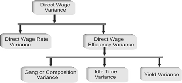
Direct wage variance
Model Steps for direct wage variances are as follows,
- L1 – actual payment made to workers for actual hours worked = Actual hours worked × Actual hourly wage rate
- L2 – estimated payment if the workers had been paid at standard rate = Actual hours worked × Standard hourly wage rate
L3 – estimated payment if workers had been used according to the proportion of standard group, and payment had been made at standard rate. Example – in actual working, Grade-I and Grade-II workers might have been used in the ratio of 75:25 instead of standard ratio of 50:50.Hence, this step will involve determining the wage payment keeping in view the following points (see Figure A2.3).
- L4 – Standard cost of labor hours utilized = Actual utilized hours × Standard hourly rate.
Note: Strike, power failure etc. should be deducted from the available hours. - L5 – Standard labor cost of output achieved = Standard labor cost per unit × Actual production.
Direct Wage Variance represents the difference between actual wages paid and standard wages specified for the production and is expressed by the difference between (L1) and (L5 ).
It is due to the difference between actual wage rate paid and the standard wage rate specified. It represents the difference between actual payment to the worker for actual hours worked (L1) and estimated payment if the worker had been paid at standard rate (L2).
Direct wage efficiency variance
It represents the difference between (L2) and (L5). It arises due to the difference between actual hours paid and standard hours allowed for output achieved. It is the sum total of labor-gang variance, labor idle time variance and labor yield variance.
Direct wage group variance
It is the difference between actual composition of the group used and standard composition specified for the group. Suppose the composition of the group changes due to a shortage of a particular grade of labor. Changing the composition of labor mix will change the efficiency of that group. The difference between (L2) and (L3) will give rise to the direct wage group (gang) variance.
Labor idle time variance
The difference between labor hours applied and labor hours utilized is the labor idle time variance difference between (L3) and (L4). The idle time variance is to be calculated when there is a difference between labor hours applied and labor hours utilized.
Labor yield variance
It is the difference between the actual output of a worker and standard output of the worker. It is also termed as the labor efficiency variance. It can be divided into two parts:
1. When there is Idle Time variance
Yield variance = Standard cost of labor hours utilized (L4 ) – standard labor cost of output achieved (L5 ).
2. When there is no Idle Time variance
In that case (L4 ) is to be considered as zero and the yield variance will be calculated from the difference between the value of (L3) and (L5 ).
Illustration – 7:
The standard composition and standard rates of a group of workers are as follows,

According to given specifications, a week consists of 40 hours and standard output for a week is 1000 units. It is observed in a particular week, a group of 13 skilled, 4 semi-skilled and 3 unskilled worked and they were paid as follows,

The production line supervisor’s report recorded that two hours were lost due to breakdown and actual production was 960 units in that week.
We have to find out –

Solution:
L1 – actual payment made to workers for actual hours worked
| Actual Composition of group | Hours worked | Rate $ | Amount $ |
| 13 skilled | 40 | 0.600 | 312 |
| 4 semi-skilled | 40 | 0.425 | 68 |
| 3 unskilled | 40 | 0.325 | 39 |
| Total | : | 419 |
L2 – payment involved if the workers had been paid at standard rate
| Actual Composition of group | Hours worked | Std. Rate $ | Amount $ |
| 13 skilled | 40 | 0.625 | 325 |
| 4 semi-skilled | 40 | 0.400 | 64 |
| 3 unskilled | 40 | 0.350 | 42 |
| Total | : | 431 |
L3 – Payment involved if workers had been used according to the proportion of standard group, and payment had been made at standard rate.
| Std. Composition of group | Hours worked | Std. Rate $ | Amount $ |
| 10 skilled | 40 | 0.625 | 250 |
| 5 semi-skilled | 40 | 0.400 | 80 |
| 5 unskilled | 40 | 0.350 | 70 |
| Total | : | 400 |
L4 – Standard cost of labor hours utilized
| Std. Composition of group | Hours utilized | Std. Rate $ | Amount $ |
| 10 skilled | 40 | 0.625 | 237.50 |
| 5 semi-skilled | 40 | 0.400 | 76.00 |
| 5 unskilled | 40 | 0.350 | 66.50 |
| Total | : | 380.00 |
L5 – Standard labor cost of output achieved
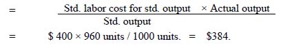
Variances

Variable overhead variance
Variable overhead per unit remain same and varies with total output (see Figure A2.4).

Variable overhead variance
Model steps are shown below,
VO1 – Actual overhead incurred.
VO2 – Actual hours worked at standard variable overhead rate
= Standard variable overhead rate per hour × Actual hours worked.
VO3 – Standard variable overhead for the production
= Standard variable overhead per unit × Actual production.
Variable overhead variance
It is the difference between actual overhead incurred during the period and standard variable overhead for production i.e. VO1 – VO3. Variable overhead variance can also be determined by taking the aggregate of variable overhead expenditure and variable overhead efficiency variance.
Variable overhead expenditure variance
It is the difference between actual variable overhead and standard variable overhead appropriate to the level of activity attempted. Variable overhead expenditure variance is the difference between VO1 and VO2.
Variable overhead efficiency variance
Variable overhead efficiency variance is the difference between actual hours worked at standard variable overhead rate (VO2) and standard variable overhead for the production (VO3).
Illustration – 8:
Following information is obtained from a pre-cast concrete slab manufacturing company for the year 1999.
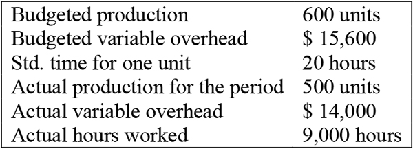
From the above data we have to find out the following variance.
- Variable overhead expenditure variance.
- Variable overhead efficiency variance.
- Variable overhead variance.
Solution
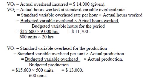
Variances
- Variable overhead expenditure variance = VO1 – VO2 = $2,300 (A).
- Variable overhead efficiency variance = VO2 – VO3 = $ 1,300 (F).
- Variable overhead variance = VO1 – VO3 = $ 1,000 (A).
A2.3.3 Fixed overhead variance

Fixed overhead variance
Fixed overhead variance arises when a company uses the absorption standard costing system. In this system, a standard rate is ascertained for fixed overheads by dividing the total fixed overhead by an appropriate base e.g. machine hours, units, labor etc. Fixed overheads incurred differ from standard allowance for fixed overheads or standard fixed overheads for production for various reasons. These give rise to different kinds of fixed overhead variances (see Figure A2.5).
FO1 – Actual fixed overhead incurred.
FO2 – Budgeted fixed overhead for the period or std. fixed overhead allowance. It represents the amount of fixed overhead which should be spent according to budget during the period. The amount of standard allowance for fixed overhead does not change due to change in volume.
FO3 – Fixed overhead for the days/hours available at standard rate during the period. It is calculated by multiplying days/hours available and standard overhead rate.
FO4 – Fixed overhead for actual hours worked at standard rate.
FO5 – Standard fixed overhead for production. It is calculated by two ways,
- Unit Method-Multiplying the actual production and standard fixed overhead rate per unit.
- Hour Method-Multiplying the actual production in standard hours and standard fixed overhead rate per hour.
Fixed overhead variance is the difference between actual fixed overhead incurred and standard cost of fixed overhead absorbed and is calculated from the difference between FO1 and FO5.
Fixed overhead expenditure variance
It is also referred to as the budget variance and arises due to the difference between actual fixed overhead incurred and budgeted fixed overhead or the standard allowance for fixed overhead. The difference between FO1 and FO2 is the fixed overhead expenditure variance.
Fixed overhead volume variance
Fixed overhead volume variance arises due to the difference between budgeted fixed overhead for the period and standard fixed overhead for actual production. This variance indicates the degree of utilization of plant and facilities when compared to the budgeted level of operation.
Fixed overhead volume variance consists of:
Calendar variance or idle time variance
Calendar variance is the difference between budgeted fixed overhead and fixed overhead for days available during the period, at standard rate i.e. the difference between FO2 and FO3.
Idle time variance is determined almost in the same way as calendar variance. The difference between FO2 and FO3 is computed in hours as per budget and hours actually available during the period.
Capacity variance
It is the difference between capacity utilized and planned capacity or available capacity. Capacity variance is calculated from the difference between FO3 and FO4. An adverse capacity variance indicates under utilization. It will lead to unabsorbed balance of fixed overhead.
Efficiency variance
Efficiency variance reflects increased or reduced output arising due to the difference between budgeted or standard efficiency and actual efficiency in utilization of fixed common facilities. It is the barometer by which management comes to know how efficiently or inefficiently fixed indirect facilities or services are being used and is the difference between FO4 and FO5.
Illustration – 9:
We have to calculate fixed overhead variances from the following cost data of Naturextracts Ltd.

Solution
Calculation of variances

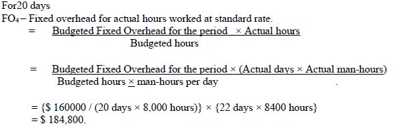
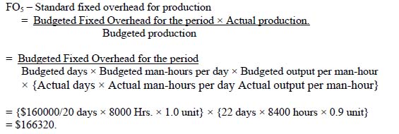
Variances
- Fixed Overhead Expenditure Variance = FO1 – FO2 = $8000 (A)
- Fixed Overhead calendar variance = FO2 – FO3= $16000 (F)
- Fixed Overhead Capacity Variance = FO3 – FO4 = $8800 (F)
- Fixed Overhead Efficiency Variance = FO4 – FO5 = $18480 (A)
- Fixed Overhead Variance= FO1 – FO5 = $1680 (A)
- Fixed Overhead Volume Variance = FO2 – FO5 = $6320 (F)
A2.3.4 Two-Variance, Three-Variance and Four-Variance Methods of Analysis
The variance analysis has already been discussed and the terms Two-Variance, Three-Variance and Four-Variance Methods are not separate methods but these terms indicate the extent to which variances are being analyzed in a particular organization.
A2.3.5 Material Cost Variances and Two-Variance, Three-Variance and Four-Variance Approach
Two-variance
The term two-variance indicates that the analysis is restricted to two factors, i.e. price and quantity only. It can be graphically illustrated as shown in Figure A2.6.
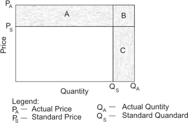
Two-variance
| Then, Actual cost | = PA QA |
| Standard Cost | = PS QS |
| Total variance | = Actual cost – Standard cost |
| = PA QA – PS QS. |
If the two-variance approach refers to material cost variance, then only material price variance and material quantity variance will be determined.
Three-variance
In this approach material cost variance, i.e. PA QA – PS QS is to be equal to A+ B + C and following variances are attempted.
a) Material price variance b) Material quantity variance c) Material mix variance.
Four-variance
The four variance approach takes the analysis still further and the area represented A+ B + C in the above figure will be divided as follows.
- Material price variance.
- Material sub-usage Variance
- Material Mix Variance.
- Material Efficiency Variance.
Overhead variance and two-variance, three-variance and four-variance approach
Overhead variance is the result of numerous contributory factors and its knowledge can be effective only when it is further analyzed according to the purposes.
Two-variance
Only expenditure variance or budget variance and volume variance are attempted under this approach.
Three-variance
The two-variance approach is viewed as inefficient for control purposes and the three-variance approach is recommended in which following three variances will be determined:
- Expenditure variance or budget variance
- Capacity variance
- Efficiency variance
Four-variance
Analysis of variances is further stretched in this approach in which calendar variance is also analyzed along with all the other three variances mentioned above.
Illustration – 10
The following figures are extracted from the books of a company:

We have to analyze the overhead variances and summarize those results according to the ‘Two-way’, ‘Three-way’ and ‘Four-way’ approach.
Solution:
Calculation of Fixed Overhead Variances
(Please refer Illustration-9 for details)
FO1 – $2500, FO2 – $2400, FO3 – $2592, FO4 – $2640 & FO5 – $2600
Variances
- Fixed Overhead Expenditure Variance = FO1 – FO2 = $100 (A)
- Fixed Overhead calendar variance = FO2 – FO3= $192 (F)
- Fixed Overhead Capacity Variance = FO3 – FO4 = $48 (F)
- Fixed Overhead Efficiency Variance = FO4 – FO5 = $40 (A)
- Fixed Overhead Variance = FO1 – FO5 = $100 (F).
- Fixed Overhead Volume Variance = FO2 – FO5 = $200 (F)
Variable overhead variance
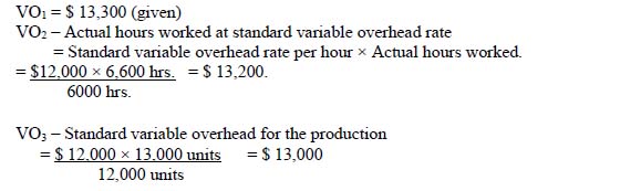
Variances
- Variable overhead expenditure variance = VO1 – VO2 = $ 100 (A).
- Variable overhead efficiency variance = VO2 – VO3 = $ 200 (A).
- Variable overhead variance = VO1 – VO3 = $ 300 (A).
The statement below shows the overhead variances under ‘Two-way’, ‘Three-way’ and ‘Four-way’ methods.

*In three-variance analysis, Fixed Overhead Capacity Variance will include Fixed Overhead Calendar Variance also.
A2.4 Non-conventional variance analysis
Internal factors, such as technological and organizational changes arise within the organization and these are controllable variances. These are normally known and planned for in advance. Extraneous factors such as inflation arise outside the organization and are uncontrollable, and require changes in a plan at short notice.
These factors invalidate the conventional variance analysis and necessitate the use of operating and planning variances.
Operating and planning variances are subsets of material total variance replacing traditional usage and price variances. These variances are used to isolate variances caused by unforeseen circumstances (planning variance) and operational variance, which reflects non-standard performance. This approach may also apply to labor and overhead.
A2.4.1 Operational/Planning variance
Operational price variance
{(Actual materials used or purchased × revised standard price) – (Actual materials used or purchased × Actual price)}.
Operational usage variance
{(Standard materials used × revised standard price) – (Actual materials used × revised standard price)}.
Planning price variance
(Standard material cost) – (Revised standard material cost).
Illustration – 11
PC & Co. has set the standard price of material at $2 per kg before the start of the period.
During the period:
- Standard quantity of material specified for the output in the period: 20,000 kg
- Actual material purchased and used: 21,000 kg
- Actual purchase price paid: $ 2.80 due to material shortage.
- At the end of the period, a price of $3 was agreed to have been an efficient buying price in the period. The standard costing system shows a direct material total variance of $18,800 made up of:
- Material usage Variance $ 2,000 (A)
- Material Price Variance $ 18,000 (A)
We need to distinguish between controllable and uncontrollable effects on performance.
Solution:
| Actual cost of purchase (21,000 × $2.8) | = $ 58,800 |
| Material actually purchased and used at revised standard cost (21,000 × $3) = $ 63,000 | |
| Revised standard cost (20,000 × $3) | = $ 60,000 |
| Standard Price: (20,000 × $2) | = $ 40,000 |
- Operational Price variance (Controllable), (a-b) = $4,200 (F)
- Operational Usage variance (Controllable), (b-c) = $3,000 (A)
- Planning Price variance (Un-Controllable), (c-d) = $ 20,000 (A)
Direct material total Variance = Planning variance + Operational variance
= 3000 (A) + 20000 (A) + 4200 (F).
= $ 18,800 (A).
Causes of different variances are given here:
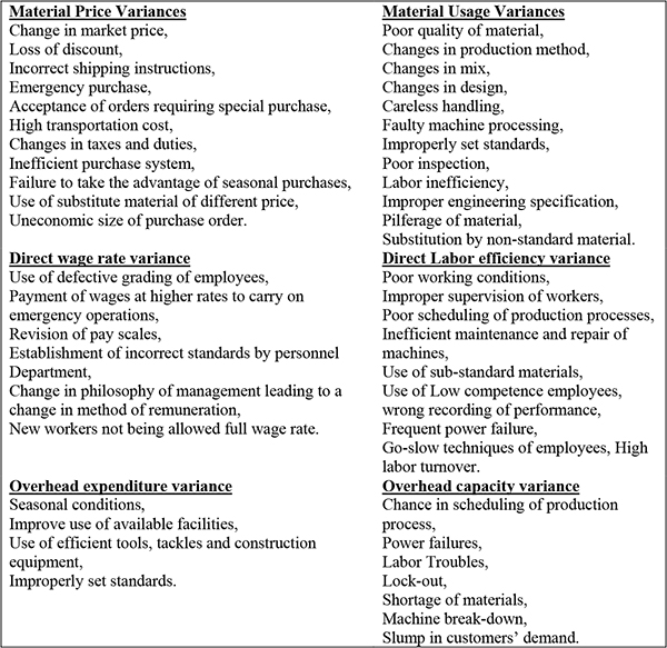

A2.5 Reporting of variances
The value of variances comes from an analysis of significant variances, the identification of their cause and the correction of these causes. The benefit of variance analysis lies in prompt communication to management and the delay may render the analysis useless. Cost control efforts are generally aided by using ratio analysis technique. The management prefers to compute a number of ratios pertaining to liquidity, profitability and capital structure etc. as opposed to absolute figures. Variance ratios Figure A2.7) help in comparing different periods and highlighting abnormalities.
The following variance ratios are commonly used:-

Variance ratios
Illustration – 12
The following data is available in the books of GKW Ltd.

The related period of 4 weeks and there was a special one day holiday due to national event. We have to calculate the following ratios: Efficiency Ratio, Activity ratio, Calendar ratio, standard Capacity Usage Ratio, Actual Capacity Usage Ratio, Actual Usage of Budgeted Capacity Ratio.
Solution:
Efficiency Ratio = 7,000 hrs. × 100 / 6,000 hrs. = 116.7%.
Activity ratio = 7,000 hrs. × 100 / 6,400 hrs. = 109.4%.
Calendar ratio = {(5 days × 4 weeks) – 1} × 100 / (5 days × 4 weeks) = 95.0%.
Standard Capacity Usage Ratio = 6,400 hrs. × 100 / 8,000 hrs. = 80.0%.
Actual Capacity Usage Ratio = 6,000 hrs. × 100 / 8,000 hrs. = 75.0%.
Actual Usage of Budgeted Capacity Ratio = 6000 hrs. × 100 / 6,400 = 93.75%.
Case studies – B
I. PRAX Inc. manufactures a single product for which the following information is available:

The following extracts were taken from the actual results and reports for two consecutive accounting years.

We have to:
- Interpret and explain every variance of Period –I showing the underlying calculations.
- Calculate the sub-variances of the fixed overhead volume variance for Period-II assuming that an alternative suggestion is adopted that such a subdivision would aid management control.
II. A jewelry manufacturing company planned to manufacture 5,000 components in the month of September. Each component requires four standard hours to complete. For the 22 working days in the month 120 workers were allocated to the job. The factory operates an 8-hours day. The worker allocation included a margin for absenteeism and idle time.
Actual results were analyzed and it was revealed that absenteeism had averaged 5%, an average of 5 hours overtime had been worked by those present and 4,800 components had been completed at an average of 3.8 standard hours each.
During October, 120 of the completed components have been scrapped because of defective material. It is also planned to produce another 5,000 units plus the shortfall from September. From the information given, you are required to:
Calculate the following ratios for September,
- The production volume ratio,
- The capacity ratio, and
- The productivity (efficiency) ratio,
Give explanation of the above results.
- Estimate the manpower required for November production using 21 working days with one hour overtime per man per day, working at the budgeted efficiency level and the same percentage of absenteeism, idle time and rejects as occurred in the September production.
- Calculate the bonus for November, on a 50:50 profit sharing basis, which could be paid as an addition to the wage rate if the September production efficiency was achieved, idle time reduced to 5% but all other features were the same as in (c) above.
A3 Cost reporting
A3.1 Common forms of reports
Narrative reports– These are descriptive and verbal reports.
Statistical reports – These reports rely on tables, numbers, graphs, charts, etc.
Periodic reports – Reports may be issued on regular scheduled basis, e.g. daily, weekly, monthly, quarterly and annually.
Progress reports – Interim reports between the start and completion of a project and also called follow-up reports.
Special reports – Generally these reports are sent irregularly in response to a specific, non-routine request. In control reports, a subordinate summarizes the activities under the jurisdiction and accounts to his superiors for results, that he has previously committed himself to achieve. The practice of ‘reporting by results’ is primarily for management control purposes.
Tabular Presentation of Cost Reports for Different Levels of Management

Top management
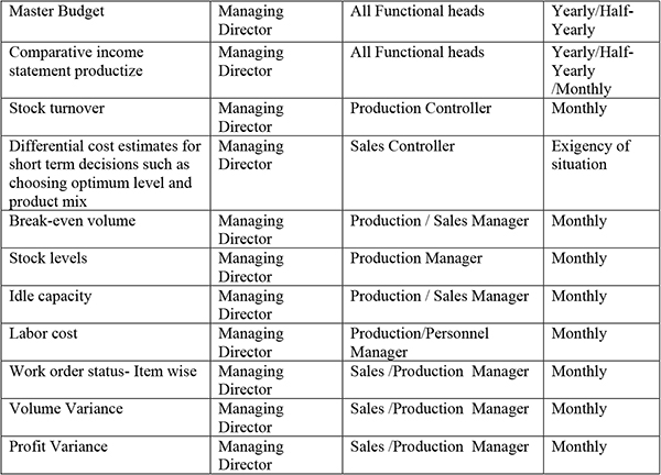
Middle Management

Operating Management


A4 Value management
The inquisitive mind is never satisfied with things as they are and is always looking at ways to make and do things better. It is considered that everything can be improved and value analysis is an outcome of this philosophy. It has been defined as an organized creative approach that emphasizes efficient identification of unnecessary cost, i.e., cost that provides neither quality, nor use, nor life, nor appearance, nor a customer’s satisfaction. It was applied as a method to improve value in existing products by Lawrence D. Miles of General electric in 1947. Initially value analysis was used principally to identify and eliminate unnecessary costs. However it is equally effective in increasing performance and addressing resources other than cost and as it evolved the application of VA widened beyond products into services, projects and administrative procedures.
Value Management (VM) has evolved out of previous methods based on the concept of value and functional approach. It is a style of management particularly dedicated to motivating people, developing skills and promoting synergies and innovation, with the aim of maximizing the overall performance of an organization.
A4.1 What is Value?
Value is a measure of how well the owner’s objectives are met. The term ‘Value’ is synonym for the term ‘worth’. Nothing can have value without being an object of utility.
A product or a service may have the following kinds of values for the customer:
- Use value – the monetary measure of the functional properties of the product or service which reliably accomplish a user’s needs.
- Esteem value – the monetary measure of the properties of a product or service which contribute to its desirability or salability. Commonly answers the ‘How much do I want something?’ question.
- Cost value – the monetary sum of labor, material, burden, and other elements of cost required to produce a product or service.
- Exchange Value – the monetary sum at which a product or service can be freely traded in the marketplace.
Value objectives
The overarching goals that define project success.
What is value management (VM)?
VM is a team based managerial approach which identifies the required performance to satisfy the business and stakeholders needs; also determines the most appropriate solutions to suit the performance. Performance includes business needs, quality, image, social benefits, and revenue generation. Value management is a collection of processes or efforts by which organizations can proactively pursue one or more identified project value objective. Traditionally, this involves a formalized team decision-making and problem-solving process.
The Value Management Approach involves three root principles:
- A continuous awareness of value for the organization, establishing measures or estimates of value, monitoring and controlling them;
- A focus on the objectives and targets before seeking solutions;
- A focus on function, providing the key to maximize innovative and practical outcomes.
A4.2 Concept of value
The concept of Value relies on the relationship between the satisfaction of many differing needs and the resources used in doing so. Value increases when customer satisfaction increases and/or expenditure of resources diminish. Resource includes time, management, design costs, capital costs, cost in use etc. The fewer the resources used or the greater the satisfaction of needs, the greater the value (Figure A2.8). Value carries different meaning for different people. Value Management helps an organization to achieve its stated goals with the use of minimum resources.

Concept of value
The value can be improved by influencing the performance and resources variables in a number of ways:

Here P and R denote functional Performance and Life Cycle Cost/ NPV respectively.
It is important to realize that Value may be improved by increasing the satisfaction of need even if the resources used in doing so increase, provided that the satisfaction of need increases more than the increase in use of resources.
A4.3 Purpose
VM is the systematic application of recognized techniques used by a multi-disciplined team to: identify the function of a product or service, establish a worth for that function, generate alternatives through the use of creative thinking, and provide the needed functions to accomplish the original purpose of the project. This should be accomplished reliably and at the lowest life-cycle cost without sacrificing safety, necessary quality, and environmental attributes of the project.
A4.4 Value methodology
The systematic application of recognized techniques which identify the functions of the product or service, establish the worth of those functions, and provide the necessary functions to meet the required performance at the lowest overall cost. The Value Methodology is a professionally-applied, function-oriented, and systematic multi-disciplined team approach used to analyze and improve value in a product, facility design, system or service. It can be applied to any business or economic sector including industry, government, construction or service. By enhancing value characteristics, VM increases customer satisfaction, and adds value to the investment.
A4.5 Function oriented approach
It is the link between the need and the product and the need is expressed in terms of performances rather than the solutions. It is a powerful methodology used for solving problems and/or reducing costs while improving value, performance, and quality.
A4.6 Cross-disciplinary team
A key to the successful application of a value study is the skill and experience of those applying the methodology and it has been proven that a well organized team obtains the best value for significant projects. The Team Leader performs a key role and is a significant factor in the degree of success and should possess strong leadership, communication skills, and experience working with users/clients. The members should represent a diverse background and experience that incorporates all the knowledge required to fully cover the issues and objectives of the project. Participant selection and stakeholders involvement is the key to success. Typically these include a Facilitator, a Client Commercial Manager, a Client Representative, an End User, a Project Manager, a Cost Manager, a Planner, a Designer, a Contractor, a Risk Manager, and Other Stakeholders.
A4.7 Structured process
Value Methodology is a structured process and consists of the following analytical and creative thought processes,
- Analyze Information
- Brainstorm Function
- Organize Function
- Generate ideas for alternatives
- Evaluate alternatives and develop proposals
- Appraise options
- Recommend solutions
A4.8 The value methodology job plan
The Value Methodology uses a systematic Job Plan (Figure A2.9). The Job Plan outlines specific steps to effectively analyze a product or service in order to develop the maximum number of alternatives to achieve the product’s or service’s required functions. Adherence to the Job Plan will better assure maximum benefits while offering greater flexibility.

The value methodology job plan
The VM Job Plan covers three major periods of activity: Pre-Study, the Value Study, and Post-Study. All phases and steps are performed sequentially.
Pre-study
Preparation tasks involve six areas;
- Collect User/Customer Attitudes
The User/Customer attitudes are compiled and the objectives are to:
Determine the prime buying influence;
Define and rate the importance of features and characteristics of the product or project;
Determine and rate the seriousness of user-perceived faults and complaints of the product or project;
Compare the product or project with competition or through direct analogy with similar products or projects. For first time projects such as a new product or new construction, the analysis may be tied to project goals and objectives. The results of this task are to be used to establish value mismatches in the Information Phase. - Accumulation of Complete Data
There are both Primary and Secondary sources of information.
Primary sources are of two varieties:
People – It includes the user, original designer, architect, cost/estimating group, maintenance service, the builders, and consultants.
Documentation –It includes drawings, project specifications, bid documents and project plans.
Secondary sources include literature such as engineering and design standards, regulations, test results, failure reports, and trade journals. Other major source is similar projects and site visit by the value study team. - Determine Evaluation Factors
The team determines the criteria for evaluation of ideas and the relative importance of each criterion to final recommendations and decisions for change. - Scope the Study
The team develops the scope statement for the specific study that defines the limits of the study based on the data-gathering tasks. - Build Models
The team compiles models for further understanding of the study after the completion of the scope statement. It includes models such as Cost, Time, Energy, Flow Charts, and Distribution, as appropriate for each study. - Determine Team Composition, Wrap-Up
The Value Study Team Leader confirms the actual study schedule, location and need for any support personnel. The Team Leader ensures that all pertinent data are available for the study.
The value study
The value study is where the primary Value Methodology is applied. The effort is composed of six stages:
- Information
- Function Analysis
- Creativity
- Evaluation
- Development
- Presentation
Information stage
The objective of the Information Phase is to complete the value study data package started in the Pre-Study Work and if a ‘site’ visit was not possible during Pre-Study, it should be completed during this phase. The purpose is to establish a common understanding of the project.
Users and stakeholders are identified in this stage. The scope statement is reviewed for any adjustments due to additional information gathered during the Information Phase. Gathering and sharing project information, background, constraints etc. are also the part of the process.
Function analysis stage
Function definition and analysis is the heart of Value Methodology. It is the primary activity that separates Value Methodology from all other ‘improvement’ practices. The objective of this phase is to develop the most beneficial areas for continuing study where project functions or objectives are analyzed to improve value, by considering: ‘What should this do?’ rather ‘What is this?’ focus on functions rather than product.
The team performs the following steps:
- Identify and define both work and sell functions of the product, project, or process under study using active verbs and measurable nouns. This is often referred to as Random Function Definition.
- Classify the functions as basic or secondary
- Expand the functions identified in step 1 (optional)
- Build a function Model – Function Analysis System Technique (FAST) diagram. The function analysis captures requirements diagrammatically into a FAST diagram which is a logical method that identifies hierarchy.
- Assign cost and/or other measurement criteria to functions
- Establish worth of functions by assigning the previously established user/customer attitudes to the functions
- Compare cost to worth of functions to establish the best opportunities for improvement
- Assess functions for performance/schedule considerations
- Select functions for continued analysis
- Refine study scope (see Figure A2.10)
FAST diagram
Creative stage
The principle objectives of the Creative Phase are to harness the multidisciplinary team’s experience and knowledge while developing a large quantity of ideas. This is a creative type of effort, totally unconstrained by habit, tradition, negative attitudes, assumed restrictions, and specific criteria. The teams are encouraged to think creatively to generate alternative ideas for achieving the project functions without judgment. The quality of each idea will be developed in the next phase, from the quantity generated in this phase.
There are two keys to successful speculation:
- First, the purpose of this phase is not to conceive ways to design a product or service, but to develop ways to perform the functions selected for study.
- Secondly, creativity is a mental process in which past experiences are combined and recombined to form new combinations. The purpose is to create new combinations which will perform the desired function at less total cost and improved performance than was previously attainable.
Methods of creative stage: Brainstorming, Crawford Slips.
Evaluation stage
The principle objective of the Evaluation Phase is to analytically judge and evaluate the ideas/options generated at the Creative Stage against the performance criteria/functions, in order to select the ideas/ options with worthwhile potential.
The process typically involves several steps:
- Eliminate nonsense or ‘thought-provoker’ ideas.
- Group similar ideas by category within long term and short term implications. Examples of groupings are electrical, mechanical, structural, materials, special processes, etc.
- Have one team member agree to ‘champion’ each idea during further discussions and evaluations. If no team member volunteers, the idea or concept is dropped.
- List the advantages and disadvantages of each idea.
- Rank the ideas within each category according to the prioritized evaluation criteria using such techniques as indexing, numerical evaluation, and team consensus.
- If competing combinations still exist, use the decision analysis matrix to rank mutually exclusive ideas satisfying the same function.
- Select ideas for development of value improvement.
If none of the final combinations appear to satisfactorily meet the criteria, the value study team returns to the Creative Phase.
Development stage
The objective of the Development Phase is to refine the key ideas/option, to select and prepare the ‘best’ alternative(s) for improving value. The data package prepared by the champion of each of the alternatives should provide as much technical, cost, and schedule information as practical. This ensures that a designer and project sponsor(s) make an initial assessment concerning their feasibility for implementation. The following steps are included:
- Beginning with the highest ranked value alternatives, develop a benefit analysis and implementation requirements, including estimated initial costs, life-cycle costs, and implementation costs taking into account risk and uncertainty.
- Conduct performance benefit analysis.
- Compile technical data package for each proposed alternative:
- written descriptions of original design and proposed alternative(s)
- sketches of original design and proposed alternative(s)
- cost and performance data, clearly showing the differences between the original design and proposed alternative(s)
- any technical back-up data such as information sources, calculations, and literature
- schedule impact
- Prepare an implementation Plan, including proposed schedule of all implementation activities, team assignments and management requirements.
- Complete recommendations including any unique conditions to the project under study such as emerging technology, political concerns, impact on other ongoing projects, marketing plans, etc.
Implementation stage
The objective of the Implementation Stage is to obtain concurrence and a commitment from the designer, project sponsor, and other management to proceed with implementation of the recommendations. This involves an initial oral presentation followed by a complete written report. As the last task within a value study, the VM study team presents its recommendations to the decision making body. Through the presentation and its interactive discussions, the team either obtains approval to proceed with implementation, or direction for additional information needed. The written report documents the alternatives proposed with supporting data, and confirms the implementation plan accepted by management. Specific organization of the report is unique to each study and organization requirements.
Post study
The objective during Post-Study activities is to assure the implementation of the approved value study change recommendations. Assignments are made either to individuals within the VM study team, or by management to other individuals, to complete the tasks associated with the approved implementation plan. While the VM Team Leader may track the progress of implementation, in all cases the design professional is responsible for the implementation. Each alternative must be independently designed and confirmed, including contractual changes if required, before its implementation into the product, project, process or procedure. Further, it is recommended that appropriate financial departments conduct a post audit to verify to management the full benefits resulting from the value methodology study.
A4.9 Value methodology applicability
Value Methodology can be applied wherever cost and/or performance improvement is desired. This method is applicable to hardware, building or other construction projects, and to ‘soft’ areas such as manufacturing and construction processes, health care and environment services, programming, management systems and organization structures. For civil, commercial and military engineering works such as buildings, highways, factory construction, and water/sewage treatment plants, as these are one-time capital projects; VM is applied from the design phase to achieve maximum benefits and is applied on a project-to-project basis. It may also be applied during the build/manufacture cycle to assure that the latest materials and technology are utilized. VM can also be applied during planning stages and for project/program management control by developing function models with assigned cost and performance parameters.
A4.10 The benefits of value management
The most visible benefits arising out of the application of VM include:
- Better business decisions by providing decision makers a sounds basis for their choice
- Improved products and services to external customers by clearly understanding, and giving due priority to their real needs
- Enhanced competitiveness by facilitating technical and organizational innovation
- A common value culture, thus enhancing every member’s understanding of the organization’s goals
- Improved internal communication and common knowledge of the main success factors for the organization
- Simultaneously enhanced communication and efficiency by developing multidisciplinary and multitask teamwork
- Decisions which can be supported by the stakeholders.
A4.11 Function analysis system technique diagram
The Function Analysis System technique (FAST) is developed by Mr. Charles W. Bytheway in 1964, and first presented as a paper to the Society of American Value Engineers conference in 1965. FAST contributed significantly to perhaps the most important phase of Value Engineering – function analysis. It is not an end product or result, but rather a beginning. It lays open the subject matter under study, forming the basis for a wide variety of subsequent study approaches and analysis techniques.
Function Analysis is a common language, crossing all technologies. It allows multi-disciplined team members to contribute equally and communicate with each other while addressing the problem objectively without bias or preconceived conclusions. As an effective management tool, FAST can be used in any situation that can be described functionally. However, FAST is not a panacea; it is a tool that has limitations which must be understood if it is to be properly and effectively used.
FAST is a system without dimensions – that is, it will display functions in a logical sequence, prioritize them and test the dependency, but it will not tell how well a function should be performed (specification), when (not time oriented), by whom, or for how much. However, these dimensions can be added to the model. Which dimensions to use is dependent on the objectives of the project. There is no ‘correct’ FAST model, but there is a ‘valid’ FAST model. Its degree of validity is directly dependent on the talents of the participating team members, and the scope of the related disciplines they can bring to bear on the problem. The single most important output of the multi-disciplined team engaged in a FAST exercise is consensus. There can be no minority report. FAST is not complete until the model has the consensus of the participating team members and adequately reflects their inputs.
The mechanics of the process
To begin the process, a basic model is offered. Figure A2.11 showing the FAST components and its parts.

FAST components
A. Scope of the problem under study
Depicted as two vertical dotted lines, the scope lines bound the problem under study, or that aspect of the problem with which the study team is involved.
B. Highest order function(s)
The objective or output of the basic function(s) and subject under study, is referred to as the highest order functions, and appears outside the left scope line, and to the left of the basic functions. Any function to the left of another on the critical path is a ‘higher’ order function
C. Lowest order function
These functions to the right and outside of the right scope line represent the input side that ‘turn on’ or initiate the subject under study and are known as lowest order functions. Any function to the right of another function on the critical path A is a ‘lower’ order function. The term ‘higher’ or ‘lower’ order functions should not be interpreted as relative importance, but rather the input and output side of the process. As an example, ‘receiving objectives’ could be the lowest order function with ‘satisfying objectives’ being the highest order function. How to accomplish the ‘satisfy objectives’ (highest order function) is therefore the scope of the problem under study.
D. Basic function(s)
Those function(s) to the immediate right of the left scope line representing the purpose or mission of the subject under study.
E. Concept
All functions to the right of the basic function(s) describe the approach elected to achieve the Basic function(s). The ‘concept’ either represents existing conditions or proposed approach. Which approach to use (current or proposed) is determined by the task team and the nature of the problem under study.
F. Objective or specifications
Objective or specifications are particular parameters or restrictions which must be achieved to satisfy the highest order function in its operating environment. Although they are not functions by themselves, they may influence the concept selected to best achieve the basic function(s), and satisfy the user’s requirements.
G. Critical path function(s)
Any function on the How or Why logic is a critical path function. If a function along the Why direction enters the basic function(s) it is a major critical path, otherwise it will conclude in an independent (supporting) function and be a minor critical path. Supporting functions are usually secondary, and exist to achieve the performance levels specified in the objectives or specifications of the basic functions, or because a particular approach was chosen to implement the basic function. Independent functions (above the critical path) and activities (below the critical path) are the result of satisfying the When question.
H. Dependent functions
Starting with the first function to the right of the basic function, each successive function is ‘dependent’ on the one to its immediate left or higher order function, for its existence. That dependency becomes more evident when the How question and direction is followed.
I. Independent (or supporting) function(s)
Functions that do not depend on another function or method selected to perform that function. Independent functions are located above the critical path function(s), and are considered secondary, with respect to the scope, nature and level of the problem, and its critical path.
J. Function
This is the end or purpose that a ‘thing’ or activity is intended to perform, expressed in a verb-noun form.
K. Activity
In recent years the activities are not normally shown on the FAST diagram, but rather used in the analysis to determine when to stop listing functions; i.e. if when defining functions the next connection is an activity, then the team has defined the functions to their lowest level. Therefore, today’s teams place the independent functions both above and below the major critical path. To those who are system oriented, it would appear that the FAST diagram is constructed backwards, because in systems terms the ‘input’ is normally to the left side, and the ‘output’ to the right. However, when a method to perform a function on the critical path is changed, it affects all functions to the right of the changed function, or stating it in function analysis terms, changing a function will alter the functions dependent upon it. Therefore, the How (reading left to right) and Why (reading right to left) directions are properly oriented in FAST logic.
Standard symbols and graphics
These symbols and graphics have become the accepted standard over the past 20 years. The four primary directions in a FAST diagram are (see Figure A2.12):
Standard symbols and graphics
The HOW and WHY directions are always along the critical path, whether it be a major or minor critical path. The WHEN direction indicates an independent or supporting function (up) or activity (down). At this point, the rule of always reading from the exit direction of a function in question should be adopted so that the three primary questions HOW, WHY and WHEN are answered in the blocks indicated below in Figure A2.13.
Standard symbols and functional directions
- HOW is (function) to be accomplished? By (B)
- WHY is it necessary to (function)? So you can (A)
- WHEN (function) occurs, what else happens? ( C ) or (D)
The answers to the three questions above are singular, but they can be multiple (AND), or optional (OR).
ALONG THE CRITICAL PATH – AND
‘AND’ is represented by a split or fork in the critical path. In both examples the fork is read as ‘AND’. In Example A, How do you ‘Build System’? By ‘Constructing Electronics) AND ‘Constructing Mechanicals.
In Example B, how do you ‘Determine Compliance Deviations?’? By ‘Analyzing Design’ AND ‘Reviewing Proposals’. However, the way the split is drawn, Example A shows ‘Constructing Electronics’ and ‘Constructing Mechanicals’ equally important; and in Example B, ‘Analyzing Designs’ is shown as being considered more important than ‘Review Proposals.’ (see Figure A2.14).

Along the critical path – ‘And’
Along the critical path – ‘OR’
‘Or’ – represented is represented by multiple exit lines indicating a choice.
Using Example A, the answer to the question, how do you ‘convert bookings’, is by ‘Extending bookings’ OR ‘Forecast Orders’. When going in the ‘Why’ direction one path at a time is followed. Therefore: ‘Why’ do we ‘Extend Bookings’? So that you can ‘Convert Bookings’. Also, why do you ‘Forecast Orders’? So that you can ‘Convert Bookings to Delivery’. The same process applies to Example B, except as in the AND Example, ‘Evaluate Design’ is noted as being less important then ‘Monitor Performance’ (see Figure A2.15).

Along the critical path – ‘OR’
‘AND’ Along the WHEN Direction
WHEN functions, applicable to independent functions and activities, AND is indicated by connecting boxes above and/or below the critical path functions (see Figure A2.16).
‘And’ along the when direction
The above example states ‘When you influence the customer’, you ‘Inform the customer’ AND ‘apply skills’. If it is necessary to rank or prioritize the AND functions, those closest to the critical path function should be the most important. It would appear that the same ‘fork’ symbol should be used to express AND in the WHEN as well as the HOW-WHY direction, giving example A this appearance (see Figure A2.17).

However, to do so would cause some graphic problems in multiple AND functions, in addition to building minor critical paths, such as (see Figure A2.18):
‘OR’ Along the WHEN Direction
OR is indicated by ‘flags’ facing right or left (see Figure A2.19).

‘OR’ Along the WHEN direction
Although Example B is an independent function (above the critical path) and Example C is activities (below the critical path), the WHEN, OR rules are equally applicable to both. Locating the ‘flags’ to the left or right of the vertical line bears on how we read back into the critical path function.
In Example C, working from below the critical path function, it reads: When you ‘request work’, you ‘order components’ OR ‘order collating’. Since the blocks are below the critical path, they are activities. In reading activities back, the flags face the HOW direction and the question reads: HOW do you ‘order Components’ OR ‘order collating’? By ‘requesting work’. Once again the graphic considerations modified the OR notations as seen on the critical path. Since OR is expressed in this form on the critical path:

It would appear that OR in the WHEN direction should follow this convention. However, the same problem in building minor critical paths from the support functions would occur. Also, the ‘flag’ OR, reading back into the critical path would be more difficult to express.

Other notations and symbols
Other notations and symbols used in expressing ideas and thoughts in the FAST Model are as follows: Indicates that the network continues, but is of no interest to the team, or does not contribute to the solution sought.

Indicates the Function (F) is further expanded on a lower level of abstraction.

Indicates that the line X connects elsewhere on the model, matching the same number.

A horizontal chart depicting functions within a project, with the following rules:
- The sequence of functions on the critical path proceeding from left to right answers the questions ‘How is the function to its immediate left performed?’
- The sequence of functions on the critical path proceeding from right to left answers the questions ‘Why is the next function performed?’
- Functions occurring at the same time or caused by functions on the critical path appear vertically below the critical path
- The basic function of the study is always farthest to the left of the diagram of all functions within the scope of the study.
- Two other functions are classified:
- Highest Order – The reason or purpose that the basic function exists. It answers the ‘why’ question of the basic function and is depicted immediately outside the study scope to the left.
- Lowest Order – The function that is required to initiate the project and is depicted farthest to the right, outside the study scope. For example, if the value study concerns an electrical device, the ‘supply power’ function at the electrical connection would be the lowest order function.
Cost Estimation Methods
Cost estimating is one of the most important steps in project management. A cost estimate establishes the base line of the project cost at different stages of development of the project. A cost estimate at a given stage of project development represents a prediction provided by the cost engineer or estimator on the basis of available data.
B1 Determining prime costs
B1.1 Introduction
From the management’s point of view, ‘What a product should have cost’ is more important than ‘what it did cost’. Reasons for deviations are rigorously analyzed and responsibilities are promptly fixed. Therefore, ‘What a product should have cost’ is a question of great concern to management for improvement of cost performance. A scientific answer based on reasons and consequences is developed by use of standard costing. Standard costing is a managerial device to determine efficiency and effectiveness of cost performance.
Standard – It is a predetermined measurable quantity set in defined conditions.
Standard Cost – It is a scientifically pre-determined cost, which is arrived at assuming a particular level of efficiency in utilization of material, labor and indirect services.
CIMA defines standard cost as ‘a standard expressed in money. It is built up from an assessment of the value of cost elements. Its main uses are providing bases for performance measurement, control by exception reporting, valuing stock and establishing selling prices.’
Standard cost is like a model, which provides the basis for comparing actual cost. This comparison of actual cost with standard cost reveals very useful information for cost control.
Standard cost is primarily used for the following purposes:
- Establishing budgets
- Controlling costs and motivating and measuring efficiencies
- Promoting possible cost reduction
- Simplifying cost procedures and expediting cost reports
- Assigning cost to materials, work-in-process and finished goods inventories
- Forms the basis for establishing bids and contracts and for setting selling prices
Standard Costing: According to CIMA (London), ‘Standard costing is a control technique which compares standard costs and revenues with actual results to obtain variances which are used to stimulate improved performance.’ Use of standard costing is not confined to industries having repetitive processes and homogeneous products only. It can be used in non-repetitive processes like manufacture of automobiles, turbines, boilers and heavy electrical equipment.

B1.2 Limitation of historical costing
- Data does not provide yardstick of comparison for actual cost
- Data is made available too late to correct inefficiencies, that are causing costs to go out of limits
- It does not provide motivation to employees to strive for accomplishment of their objectives
- Data provides insufficiently for budgeting, planning, decision making and price quotation
These limitations of historical costing are primarily responsible for the advent and wide usage of standard costing.
B1.3 Advantage of standard costing
General advantages
- Use of standard costing leads to optimum utilization of men, materials and resources
- Its use provides a yardstick for comparison of actual cost performance
- Only distinct deviations are reported to management. It helps in the application of the principle of ‘management by exception’
- It is useful to management in discharging functions, like planning, control, decision making and price fixing
- It creates an atmosphere of cost consciousness
- It motivates workers to strive for accomplishment of defined targets
- It highlights areas, where a probe promises improvement
- Its introduction leads to simplification of procedures and standardization of products
- It reduces the time required for preparation of reports for pricing, control or quotation purposes
- It helps determine the cost of finished goods immediately after completion
- This eliminates much clerical effort in pricing, balancing and posting on store ledger cards and stock ledgers can be maintained in terms of quantities only
- Its use may encourage action for cost reduction.
Specific advantages
Specific uses of standard costing in an organization are summarized below:
Accounting department is benefited by:
- Planning and budgeting, valuation of inventories, cost control, pricing, sales and cost estimates, developing monthly operating results.
Production department is benefited by:
- Production planning, matching scheduled production with machine capacity and preparing reports of business logs in terms of time
Sales department is benefited by:
- Determining and checking selling prices, preparing quotations on special products and determining the profitability of specific product lines
B1.4 Preliminaries to establishment of standards
Before standard cost for different elements is determined, management should take a decision about the following:
- Length of period of use
- Types of standard to be used
- Review of existing procedures
- Classification of accounts
- Review of existing coding system
B1.4.1 Types of standards
Based upon tightness, looseness and period of operation, standards have been classified in the following categories:
Based on period of operation
- Current standards
- Basic standards
- Normal standards
Based on tightness and looseness
- Ideal standards
- Expected or attainable standards
B1.4.2 Setting of standards
Determination of standards for various elements of cost is an exercise, which requires skill, imagination and experience. The job of setting the standards is done by a group, which is represented by Engineering, Production, Purchase, Personnel and Cost Accounts department. Setting of standards can be divided in two categories:
- Determination of quantity standards
- Determination of price standards
Prime cost (direct material and direct labor) – is determined by the multiplication of a physical factor by a monetary factor. The physical factor is the quantity purchased (1000 units) and the monetary factor is the price paid ($1.10 per unit). The multiplication of the two produces an actual material cost of $1,100 for this item.
B2 Overhead allocation
B2.1 Introduction
A cost item may have a direct or indirect relationship with the cost objective, i.e., the purpose or object for which the cost is being ascertained. Based on the direct and indirect relationship of the cost object, the total cost is supposed to be composed of the following two major categories: Prime and Overhead costs.
All direct costs are part of the prime cost, which is an aggregate of direct material cost and direct wages. All indirect costs form a part of the overhead, which is an aggregate of indirect material cost, indirect wages and costs of indirect services. Therefore overhead is a pool of indirect costs, i.e., the costs which cannot be identified or linked or attributed or allocated to the cost objective. CIMA defines overhead/indirect cost as expenditure on labor, materials or services which cannot be economically identified with a specific saleable cost per unit. The concept of overhead is shown in Figure B2.1.

The overhead concept
When traceability is the basis of cost classification, the terms direct costs and indirect costs are used. On the other hand, if cost is classified based on elements, prime cost and overhead are used. Overhead may include some direct costs, which are so small in amount, that it will be inexpedient to trace them to specific units of production. Screws, bolts, glue etc., are a few examples. These items can be directly traced to cost units, but the cost involved may be so insignificant that it would be inexpedient to do so.
B2.2 Elements of overhead
Indirect material cost
Indirect material cost is that material cost which cannot be assigned to specific units of production; it is common to several units of production. A few examples of these are consumable stores, lubricating oil, cotton waste and small tools for general use. Sometimes indirect material cost includes direct material cost, which is so small or complex that direct tracing to specific units is inexpedient; for example, glue, thread, rivets, chalk etc.
Indirect labor cost
Indirect labor cost is that portion of labor cost, which cannot be assigned to any specific units of production; it is common to several units. Salaries of a foreman, supervisory staff and works manager, wages for maintenance workers, idle time, and workmen compensation are some of the examples of indirect labor cost. These, like some direct material cost, are not assigned to the specific units of production for the sake of expediency. Employees’ social security charge and unemployment payroll taxes are the two examples that fall under this category.
Indirect services cost
A few examples of indirect services are:
- Repair and maintenance of plant and machinery
- Factory rent
- Expenses of keeping and handling of stores
- First aid expenses
B2.3 Classification and collection of overhead
Classification is the process of grouping according to common characteristics. Overhead is classified on the basis of functions, behavior and elements.
B2.3.1 Function-wise classification
Overhead can be divided into the following categories based on functionality:
- Manufacturing overhead, Administration overhead, Selling overhead, and Distribution overhead
Manufacturing overhead
The term manufacturing stands for activities, which begin with the receipt of an order and end with the completion of the finished product. Manufacturing overhead represents all manufacturing costs other than direct material and direct labor. These costs cannot be identified specifically with or traced to a cost object in an economically feasible way. There is a growing tendency to prefer the term indirect manufacturing cost to overhead. Given below are a few examples of different items included in different groups of manufacturing overhead:
- Indirect material cost – Glue, thread, nails, rivets, lubricants, cotton waste etc
- Indirect labor cost – salaries and wages of foreman and supervisors, inspectors, maintenance, labor, general labor, idle time etc
- Indirect services cost – Factory rent, factory insurance, depreciation, repair and maintenance of plant and machinery, first-aid, rewards for suggestions for welfare, repair and maintenance of transport system and apportioned administrative expenses etc.
Administration overhead
The term administration stands for formulation of policy, direction, control and management of affairs. Administration overheads include the indirect costs incurred for the general direction of an enterprise as a whole. It encompasses the cost of management, secretarial, accounting and administrative services, which cannot be related to the separate production, marketing or research and development functions.
Given below are a few examples of different items included in different groups of manufacturing overhead:
- Indirect material cost – printing and stationery for administration
- Indirect labor cost – salaries of administrative directors, secretaries and accountants, salaries of cash credit department; salaries of taxation department etc
- Indirect services cost – rent, rates and insurance of general office, bank charges, telephone, heating, cleaning of general office, building and equipment, legal fees etc. related to administrative functions.
Selling overhead
Selling overheads include only indirect costs relating to selling which is a separate function like manufacturing, administration and distribution. Given below are a few examples of different items included in different groups of selling overheads:
- Indirect material cost – Printing and stationary for selling, mailing literature, catalogues, price lists, samples, free gifts, displays and exhibition material etc
- Indirect labor cost – Salaries and commission of salesmen, technical representatives and sales managers and salaries of selling department etc
- Indirect services cost- advertisement expenses, bad debts, collection charges, rents, rates and insurance of showrooms, cash discount, after-sales service, brokerage, expenses in making quotation etc
Distribution overhead
Distribution overheads include indirect costs relating to distribution, which is a separate function like manufacturing, administration and selling. The term distribution stands for activities connected with sequence of operations that start from making the packed product available for dispatch and end with making reconditioned returned empty package available for reuse.
Given below are a few examples of different items included in different groups of distribution overhead:
- Indirect material cost – Packing cases, oil, greases, spare parts etc. for upkeep of delivery vehicles
- Indirect labor cost – Wages of packers, van drivers, dispatch clerk etc
- Indirect services cost – Carriage and freight outwards, rent, rates and insurance of warehouses, maintenance of transport vehicles and running expenses of the same etc
B2.3.2 Behavior-wise classification
This classification is important for accounting and control. Based on behavioral patterns, overhead can be divided into the following categories: Fixed overhead, Variable overhead and semi-variable overhead.
Fixed overhead
Fixed overhead represents indirect cost, which remains constant in total within the current budget period regardless of changes in volume of activity. This concept of fixed overhead remains valid within certain output and turnover limits. Fixed overhead does not vary in total. The incidence of fixed overhead on unit cost decreases as production increases and vice versa (rent of building, depreciation of plant and machinery and building, cost of hospital and dispensary, pay and allowances of managers, secretary and accountants canteen expenses, legal, fee, audit fee etc). Fixed cost will be incurred even when no production activity takes place (see Figure B2.2).

Fixed overhead
Fixed overhead per unit is changing (decreasing with increase in volume), total fixed overhead is constant.
There are three types of fixed overhead:
- Long-run capacity fixed overhead – these are the expired cost of plant, machinery and other facilities used
- Operating fixed overhead – these overheads are incurred to maintain and operate the fixed assets; heat and light, insurance and property taxes are examples of fixed overhead of this category
- Programmed fixed overhead – these are cost of special programs approved by management. The cost of extensive advertising and cost of programs to improve the quality of the firm’s products are examples of programmed fixed overhead
Fixed overhead is fixed within specific limit relating to time and activity. Fixed overhead is dependent on the policy of management and the company’s activities. Policy of a particular management may be opposed to discharging supervisors during lean periods. Accordingly, supervision will be a fixed overhead.
Variable overhead
Variable overhead represents that part of indirect cost which varies with change in the volume of activity. It varies in total but its incidence on unit cost remains constant.
The examples of variable overhead are indirect material cost, indirect labor cost, power and fuel, internal transport, lubricants, tools and spares (see Figure B2.3).

Variable overhead
Total variable overhead is increasing whereas variable overhead per unit is constant.
Semi-variable overhead
It is that part of overhead which is partly fixed and partly variable. These overheads show mixed relationship, when plotted against volume. Semi-variable overheads may remain fixed within a certain activity level, but once that level is exceeded, they vary without having direct relationship to volume changes. It does not fluctuate in direct proportion to volume. An example of semi-variable overhead cost is the earning of an employee, who is paid a salary of $500 per month (fixed) plus a bonus of $0.5 for each unit completed (variable). If he increases his output from 1000 units to 1500 units, his earnings will increase from $1000 to $1250. An increase of 50% in volume brought about only 25% increase in cost.
Figure B2.4 shows the behavior pattern of semi-variable overhead.
Semi-variable overhead
Semi-variable overheads present the biggest problem in cost analysis because there is a readily ascertainable relationship between cost and volume. Semi-variable overhead must be segregated into fixed and variable element. The following are methods of estimating fixed and variable components.
Intelligent estimate of individual items
In this method, past overhead data relating to various activity levels are analyzed and tabulated to show the pattern of overhead relationship with volume. Suitable adjustments are made for anticipated changes. This approach is simple and inexpensive, but its simplicity is its inherent weakness. This method lacks scientific basis required for decision making.
High and low method
It is also known as Range method. Here, levels of highest and lowest expenses are compared with one another and related to output attained in those periods. Since the fixed element of semi-variable overhead is expected to remain fixed for two periods, it is concluded that changes in levels of expenses are due to variable elements. Variable cost per unit is calculated as follows,
Change in expenses corresponding to these levels should be divided by changes in output levels.
Illustration-1:

Considering highest and lowest levels of output:

Only variable cost will change,
Variable cost per unit = $13,200/4,400 units = $3 per unit.
Fixed cost will be = $ 38,200 – (9,400 × $ 3) = $10,000.
This method of segregating semi-variable overhead in their fixed and variable components is not good, because it lacks scientific basis required for decision making.
Method of averages
Under this method, averages of two selected groups are first taken and then the high and low method is followed to separate the fixed and variable components of semi-variable overhead. The method is explained below:

Variable cost = $ 1,650/ 550 units = $3 per unit.
Fixed overhead = $ 32,200 – (7400 × $ 3) = $10,000.
This method suffers from all the limitations of the high and low method.
Analytical method
In this method, the degree of variability is found out for each item of semi-variable expense. With this information, variable and fixed components for each item are separated.
E.g. Semi-variable overhead for October is $300. Variability element 60%. Variable element will be $180 and fixed element will be $120.
It does not present scientific basis and determining variability may be influenced by personal bias.
Scattergraph method
This is the statistical method, where a line is fitted to a series of data by observation. It is explained below:
Illustration-2:
Drawing a line of best fit from the following data


Scattergraph diagram
The scatter graph is a simple method requiring no complicated formulae (see Figure B2.5). It shows cost behavior pattern graphically and is easily understood. It has one serious limitation: fitting the trend line may be influenced by personal bias. The advantage of this method is speed and simplicity rather than accuracy.
Least square method
Under this method, ‘line of best fit’ is drawn for a number of observations with the help of a statistical method. Here, the straight line formula, y = mx + c, where x and y are degree variables, m and c are constant. C is the fixed element of cost, and m is the degree of variability.
Thus for each period,
y1 = mx1 + c
y2 = mx2 + c
yn = mxn + c
By addition, Σy = mΣx + Nc ……………………………………………(i)
Again, multiplying both sides of linear equation y = mx + c by x, we get
x1y1 = mx12 + cx1
x2y2 = mx22 + cx2
xnyn = mxn2 + cxn
By addition, Σxy = mΣx2 + cΣx…………………………………………(ii)
From (i) & (ii) value of constant m and c can be obtained and a pattern of cost line can be determined accordingly. Once m and c are known both x and y can be found out.
Illustration-3:

We have to find out the regression line by least square method. What will the semi-variable overhead be in July if production level increases to 500 units?
Solution
We know,
Σy = mΣx + Nc ……………………………………………(i)
Σxy = mΣx2 + cΣx…………………………………………(ii)
Substituting the above (i) & (ii),
210 = 1800m +6c………………………………………… (iii)
67,000 = 580000 m + 1800c………………………………..(iv)
By multiplying (iii) with 300,
63,000 = 540000 m + 1800 c…………………………………(v)
From (iv) and (v), m = 0.10
Putting the value of m in (iii), c = 5
Putting the values of constants m and c the equation line reduces to y = 0.1x + 5.
This is the regression line of best fit, where y = semi-variable overhead;
X = volume of production.
If x = 500, y = 0.1(500) + 5 = 55.
Thus, if production level is 500 in July, semi-variable overhead will be $55.
Limitations of the ‘Line of best fit’
The most important limitation of this method is the assumption that there is an ongoing stable relationship between costs and volume of activity. Therefore, with the increase of both cost and volume it cannot be inferred that a rise in cost has been necessarily caused by an increase in volume.
B2.3.3 Manufacturing overhead
Manufacturing overhead represents all costs incurred in the factory over and above direct material cost and direct labor cost. It is the aggregate of factory indirect material cost, factory indirect labor cost and cost of factory indirect services.
Examples of these costs are: consumables stores, lubricating oil, factory rent, repairs and maintenance of plant and machinery, depreciation of plant and machinery used in the factory, depreciation of factory building, etc.
B2.3.4 Distribution of overhead
The relationship between items of overhead and their object cannot always clear. Due to this difficulty the distribution of overhead has become a complex problem for the cost accountant.
Three aspects of this problem are shown below:
- Distribution of overhead among production departments and service departments, i.e. primary distribution
- Distribution of cost of service departments among production departments, i.e. absorption of overhead
- Absorption of production department’s overheads by units produced (see Figure B2.6).

Distribution of overhead
It is shown here that items of overhead are distributed in production departments and service departments disregarding their distinction (see Figure B2.7(a) and (b)).

Under secondary distribution, cost of service departments is distributed among production departments.

The above figure shows that absorption of overhead involves distribution overhead of production departments in units produced.
For the purpose of assignment and distribution, the following terms are relevant:
Allocation – the process identification of whole items of overhead to specific departments is termed as allocation. The item of overhead cannot be identified with specific units of production, but with the specific department for the purpose of allocation. For example, the material issued to the repair department cannot be linked with specific units of production, but this item of overhead can be allocated directly to the maintenance service cost center. An item of overhead cannot be allocated to a department, till the two following conditions are satisfied,
- The concerned department should have caused the overhead item to be incurred
- The exact amount of overhead should be known. Original records contain a lot of information to enable the different items of overhead to be allocated to specific departments. It is illustrated in the following table,

Apportionment – The items of overhead, which cannot be identified with specific departments, are prorated or distributed among the related departments and this prorating of distribution is technically referred to as apportionment.
Cost Attribution – It is a process of relating cost to cost center or cost units using cost allocation or apportionment.
Primary distribution of overhead – Primary distribution involves allocation or apportionment of different items of overhead to all departments of the factory. In primary distribution, the distinction between the production and the service department is disregarded. The following points are to be followed for apportionment of items for primary distribution.
- Basis adopted for apportionment for primary distribution should be equitable and practicable
- Charges should be made to different departments in relation to benefit received
- Method adopted for primary distribution should not be time consuming and costly
The following bases are most commonly used for apportioning items of overhead among production and service departments for primary distribution.

Illustration-4:
The SQC & Co. is divided into four departments. A, B, C are production departments and D is a service department. The actual costs for the period are as follows:

The following data of four departments is available

Apportion the costs of the various departments on most equitable basis.
Solution:
Departmental Distribution Summary

Secondary distribution
The process of redistributing the cost of service departments among production departments is known as secondary distribution. The distinction of production departments and service departments dominates secondary distribution.
Criteria for secondary distribution
The available basis for determining the basis for apportionment of cost service departments among production department.
- Services received
- Analysis of survey or survey of existing conditions
- The ability to pay basis
- Efficiency or Incentive Method
- General use indices
Common bases for secondary distribution
The representative lists of bases, which are frequently used for apportioning cost of service departments among production departments, are shown below;

B2.3.5 Methods of redistribution
Once the basis for redistribution of service department cost has been determined, actual redistribution can be done by any of the following methods (see Figure B2.8):
Secondary distribution overhead
Direct redistribution method
In this method, service departments’ costs are apportioned to production departments (only) ignoring service rendered by one service department to the other. Here, the number of secondary distribution will be equal to number of secondary departments.
Illustration 5:
PJ & Co. Ltd. has three production departments and four service departments. The expenses for these departments as per the primary distribution summary were the following:

The following information is also available in respect of the production departments:
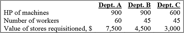
Solution:

Step method
It is a method of secondary distribution on non-reciprocal basis. It gives cognizance to the service rendered by one service department to another service department. In this method, there is no two-way distribution of costs between two service departments. E.g., a portion of power plant cost may be distributed to the tool room, because power plant provides service to tool room. But no part of the tool room cost is distributed to the power plant, even if the tool room renders service to it. The cost of service department, which serves the largest number of other departments, is distributed first. After this, the next largest number of department is apportioned and goes on till the cost of the last service departments is apportioned among production departments only.
Illustration 5:
A manufacturing company has two production departments, X and Y, and three service departments – stores, time-keeping and maintenance. The departmental distribution summary showed the following expenses for January 2003.
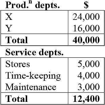
Other information relating to these departments was:

Apportion the cost of service departments to production departments keeping in view that the company makes secondary distribution on non-reciprocal basis.

Note:-
1. Bases taken for apportionment of cost of various service departments are
- Time keeping – no. of employees (2:1:4:3)
- Stores – no. of stores requisitions (3:12: 10)
- Maintenance – machine hours (4: 2).
2. It is concluded from the given information that
- The Time-keeping department serves the largest number of departments
- The Stores department serves the next largest number of departments.
Reciprocal service method
This method is applicable when there are two or more service departments and each one may render service to others. These inter-departmental services are considered while distributing expenses of service departments. This reciprocal basis for secondary distribution method facilitates cost control of the service department.
Three methods available for dealing with reciprocal services:
a) Trial and Error method
In this method, cost of one service department is apportioned to another service department. The cost of another service department plus the share received from first service department is again apportioned to first service department and this process is continued till balancing figure becomes negligible.
Illustration 6:
Data assumed cost of service of Department X and Y are $2,000 and $2,400. The analysis reveals that department X renders 30% of its services to department Y and Y department renders 20% of its services to X department. We have to show how reciprocal distribution of cost is taking place between two departments.
Solution:

The cost of Dept. X and Y will be $2,638.29 and $3,191.49 respectively.
Repeated distribution method
It is also known as continued distribution of attrition method and service department costs are distributed to other service departments and production departments on agreed percentages. This process continues to be repeated, till the figures of service departments are too small to be considered for further apportionment.
Illustration 7:
Clive & Co. has three production departments and two service departments. Departmental distribution summary for the month of January 2003 is given below.
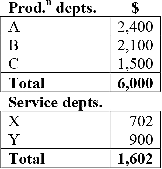
The expense of service departments are charged on a percentage basis as follows:

Distribution of service department cost under repeated distribution method has to be ascertained.
Solution:
Secondary Distribution Summary
January 2003

The last step will involve insignificant approximation.
Simultaneous equation method
Under this method true costs of service departments are first ascertained with the help of simultaneous equations. These are then distributed among production departments on the basis of given percentages.
Illustration 8:
Let us consider the same data for this case also. We have to prepare a statement showing the apportionment of two Service Department’s expenses to Production Departments by Simultaneous Equations Method.
Solution:
Let, P = total overhead of department X
N= total overhead of department Y
or P = 702 + 20/100N, and N = 900 + 10/100P.
or 10P-N =7020, and 10N – P = 9000.
Thus, P = 800 and N = 980.
We can now apportion the total overhead,

B2.4 Overhead absorption
Overhead absorption is an exercise by which overheads are properly spread over to production for the period. The selection of the correct method of overhead absorption is very important for pricing, tenders and other managerial decisions. Overhead absorption is accomplished by overhead rates.
B2.4.1 Overhead absorption rates
Absorption rate is a rate charged to the cost unit intended to account for the overhead at a predetermined level of activity. The amount of overhead divided by total number of units of the base selected such as direct labor hours; machine hours, production units etc.

The overhead absorbed in a period will be found out by multiplying overhead rate by total number of units of the base for the period.
The main objectives of determining overheads rates are given below,
- Helps to compute the amount of overhead to be included in unit cost.
- Cost compilation can be done immediately after the production.
- It determines the amount to be debited to WIP account for indirect material, indirect labor and indirect expenses for production.
- It estimates the overhead cost to be included in unit cost in advance of production.
Different types of overhead rates are briefly discussed in the following section.
Actual overhead rate
It is known as the historical overhead rate and is determined as follows:

The disadvantages of the use of the actual overhead rate are as follows,
- Actual overhead rate cannot be determined until the end of the period.
- Seasonal and cyclical influences cause wide fluctuations in actual overhead cost and actual volume of activity.
- Due to frequent changes in product cost, the cost comparison for different periods is very difficult.
Pre-determined overhead rate

Advantages:
- Pre-determined overhead rate facilitates product cost determination immediately after production is completed.
- In this case overhead cost is not distorted by seasonal or cyclic fluctuations.
- It is useful when cost-plus contracts are under taken.
- Cost estimating and competitive pricing offer ideal situations for use of predetermined overhead rates.
Predetermined overhead rates may be determined with any of the bases – previous year’s experience, expected performance, probable future performance, and optimum operating conditions.
Supplementary overhead rates
When predetermined overhead rates are used, a difference arises between overhead absorbed and overhead incurred. This under or over-absorbed overhead divided by base (number of hours, dollars or units) gives a supplementary overhead and is used to carry out adjustment between overhead absorbed and overhead incurred. It is used in addition to some other rates.

Advantages:
- It facilitates absorption of actual overhead incurred for production.
- Actual overhead rates produce erroneous results necessitating use of supplementary overhead rates.
- Where normal overhead rates are in operation, supplementary overhead rate gives good additional cost information of comparison.
Disadvantages:
- These rates can be determined only after the end of the accounting period.
- Use of supplementary rates requires a lot of clerical labor and cost.
- Where normal rates are used application of supplementary rate defeats the basic concept of normal cost.
Normal overhead rate
This overhead rate is based on the concept that actual cost is not necessarily the best criterion of true cost. Proper overhead will be charged to production, when overhead rate is linked with normal capacity i.e., normal overhead rate is a pre-determined rate determined with reference to normal capacity.

Blanket overhead rate
This is known as plant-wise or the single overhead rate for the entire factory.

Disadvantages:
- It invites too much of averaging
- A single overhead rate for the whole factory ignores the differences among production departments
Advantages:
- It is easy and convenient to use for making quick estimates.
- It is most useful in companies producing a main product in continuous processes, e.g., chemical plant, glass factory etc.
- Blanket rate may be used where several products are made, provided:
- All products pass through all departments,
- All products utilize the same amount of time in each department and
- The ratio of one product to another product remains constant.
Multiple overhead rates
If the blanket rate is not found satisfactory, a company uses multiple overhead rates in which the overhead rate is sub-divided into two or more parts for accurate product costing. Sub-division of overhead may be done on any one or more of the following lines:
- Separate rate for each production department.
- Separate rate for each service department.

Overhead rates for service departments are used when secondary distribution is not done, i.e., costs of service departments are not allocated or apportioned to production departments.
• Separate rate for each cost center
These rates are useful in making a comparative study of cost behavior of different
cost centers.

• Separate rate for fixed and variable overhead

• Separate overhead rate for each product line.

• Separate rates for applying the material-related part, the labor-related part and the facility-related part of overhead cost.

Capacity and overhead rate
Maximum plant capacity – the ideal capacity for which plant is designed to operate. It is a theoretical capacity and does not give allowance for waiting, delays and shut-down. For cost consideration, this capacity is not important.
Practical capacity – it is the maximum theoretical capacity with minor unavoidable interruptions like time lost for repairs, inefficiencies, breakdown, delay in delivery of raw materials and supplies, labor shortages and absence, Sundays, holidays, vacation, inventory taking etc. Normal unavoidable interruptions account for 15-25% of the maximum capacity.
Normal Capacity – idle capacity due to long-term sales trend only is reduced from practical capacity to get normal capacity. It is determined for the business as a whole. For normal capacity determination, prime considerations are physical capacity and average sales expectancy. It is important for budget preparation, standard cost calculation, overhead rate determination etc.
The Figure B2.9 given below clarifies the above basic capacity concept.

Basic capacity concept
Capacity based on sales expectancy- The capacity based on sales expectancy may be fixed to be either above normal capacity or below normal capacity. It is always less than practical capacity (see Figure B2.10).

Capacity based on sales expectancy
While normal capacity considers the long-term trend analysis of sales, which is based on sales of a cycle of years, the capacity based on sales expectancy is based on sales for the year only. It is influenced more by general economic conditions and forecast of industry than long term sales trends. The main advantages of determining overhead rate based on sales expectancy are:
- Overhead rate is linked with actual sales expectancy,
- Overhead costs are adequately spread over the production and
- Overhead rate determined for this purpose is very useful for making price fixation, etc
Idle capacity and excess capacity – the difference between practical capacity and normal capacity, i.e., the capacity based on long-term sales expectancy is the idle capacity. If actual capacity happens to be different from capacity based on sales expectancy, the idle capacity will be the difference between practical capacity and actual capacity. Idle capacity is that part of practical capacity which is not utilized due to factors like temporary lack of orders, bottlenecks and machine breakdown, etc and is different from excess capacity.
Excess capacity refers to that portion of practical capacity which is available, but no attempt made to for its utilization for strategic or other reasons. It is also results from imbalance or bottlenecks in certain departments. Overhead rate includes cost of idle capacity; excess capacity is excluded from overhead rate consideration.
Illustration 9:
Modern Electricals Ltd. manufactures motor engine parts at the rate of 2 units per hour. The factory normally operates 6 days a week on a single eight- hour shift. During the year it is closed on 16 working days due to holidays. Equipments are idle for 160 hours for cleaning, oiling, etc. Normal sales demand averages 3,000 units over a year a five-year period. The expected sales volume for the year 2003 was 2,800 units. Capacity actually utilized in 2003 turned out to be 1,400 units. The fixed cost is $ 110,376 per year. We have to calculate the idle capacity costs assuming that overhead rates are based on maximum capacity, practical capacity, normal capacity and expected actual capacity respectively.
Solution:

Statement showing idle capacity and machine hour rate for 2003
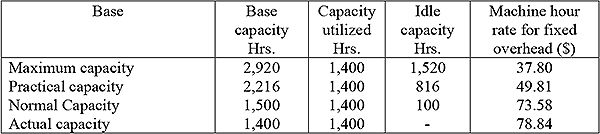
Statement showing the idle capacity costs

B2.5 Methods of absorption
Production Unit Method – Actual or predetermined overhead rate is calculated by dividing the overhead to be absorbed by the number of units produced or expected to be produced.
Advantage: It is very good for concerns having single product output.
Disadvantage: Not suitable for different products. It is neither time based nor time-related.
Percentage on Direct Wages – This percentage is determined by dividing the overhead to be absorbed by direct wages and multiplying the result by hundred.
Advantage: It is very simple and economical. Labor can be better basis than material for determining overhead.
Disadvantage: Ignores contribution made by other factors of production like machinery. It ignores time-related overheads such as taxes, insurance and depreciation. It is not related to the efficiency of a worker.
Percentage on Direct Material Cost – This percentage is computed by dividing the overhead to be absorbed by direct material cost incurred or expected to be incurred and multiplying the result by hundred.
Advantage: It is simple and easy to understand. This method is useful, when grades of materials and prices of materials do not widely fluctuate and material cost forms a major part of total cost.
Disadvantages: There exists no logical relationship between items of manufacture, overhead and material cost. It ignores the items of overhead linked with time factor, such as rent, etc. This percentage method is inequitable, when a part of the material passes all processes and a part of material passes only through some processes. If prices differ widely, the products made from materials with high prices will be charged with more than their share of overhead.
Percentage on Prime Cost – The percentage is computed by dividing the overhead to be absorbed by prime cost incurred or expected to be incurred and multiplying the result by hundred.
Advantages: Simple and easy to use, since all the data is available and no additional information is required. It is useful in those cases, where there are no wide fluctuations in processing.
Disadvantages: No logical relationship between items of overhead and prime cost. It ignores the items of overhead linked with time factor. The use of prime cost for determining the overhead rate further confuses overhead absorption.
Direct Labor Hour Method – When this method is used, actual pre-determined overhead rate is determined by dividing the overhead to be absorbed by labor hours expended or expected to be expended. It is a time based method of overhead absorption and is sometimes preferred to the direct wage method.
Advantages: It is very useful for labor intensive situations and not affected by output related remuneration schemes.
Disadvantages: This method ignores other factors of production like machines and will not be a good method of overhead absorption where machines represent the prime production factor. It requires collection of additional data, (hours worked) translating into extra clerical labor and cost.
Machine Hour Rate – When this method is used, actual or predetermined overhead rate is calculated by dividing overhead to be absorbed by the number of hours for which a machine or machines are operated or expected to operate. It is used when production is machine based and recognized as the most reliable method of overhead absorption.
The machine hour rate is of three types:
Ordinary Machine Hour Rate – It is calculated by taking into account all the indirect expenses which are directly attributable to the machine. Expenses fall into two categories.
- Proportionate to the running time of the machine i.e., power, fuel, repairs and maintenance and depreciation, known as machine expenses.
- Not having any relation to operating time i.e. insurance, taxes, lubricants etc.
Composite Machine Hour Rate –This rate takes into account not only the expenses directly connected with the machine as mentioned earlier, but also other expenses like supervision, rent, lighting, heating, etc. These indirect expenses are known as standing charges. Hence standing charges plus ordinary machine hour rate gives the composite machine hour rate.
Group Machine Hour Rate – It is determined for a cost center which comprises a specific machine or a group of machines. This method is applicable where identical machines are grouped as a machine center such as a turning shop, milling shop, drilling shop, welding shop, etc. All direct expenses are allocated to the cost center and all indirect expenses are apportioned to each group of machines on an appropriate basis.
Illustration 9:
We have to find out the machine hour rate for the month of Jan, 2003, to cover overhead expenses given below (relating to a machine).
Per annum
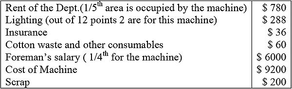
It is assumed that the machine will run for 1800 hrs. per annum and that it will incur $1,125 for repair and maintenance for life. It is also considered that the machine requires 5 units of power per hour available at 6 cents per unit and that its life will be of 10 years.
Solution:

Sales Price Method – In this method, actual overhead rate or predetermined overhead rate is determined by dividing the overhead to be absorbed by the sales realized or expected to realize. The sale price method is considered very useful for absorption of administration overhead and selling and distribution overhead.
Under or over absorption of overheads – When pre-determined overhead rate is used there happens to be a difference between the overhead absorbed and the overhead incurred during the period under consideration. If the overhead absorbed is less than the overhead incurred, the excess incurred is termed as unabsorbed overhead. If overhead absorbed or overhead charged is more than the overhead incurred during the period, the excess absorbed over incurred is termed as over-absorbed overhead.
The following methods are often used to disposing under-over/absorbed overheads.
- Adjustment to cost of sales
- Write off to profit and loss account
- Adjustment to gross profit
- Use of reserve account
- Adjustment of cost of sales and inventories
B2.6 Case studies
I. P Ltd. manufactures four brands of toys A, B, C, and D. If the company limits the manufacture to just one brand the monthly production will be:
A – 50,000 units, B – 1, 00,000 units, C – 1, 50,000 units, D – 3, 00,000 units.
We have the following set of information from which we have to find out the brand wise profit or loss clearly showing the following elements:
- Direction Cost,
- Works Cost,
- Total Cost.

Factory overhead expenditure for the month was $162,000. Selling and distribution cost should be assumed @ 20% of works cost. Factory overhead expenses should be allocated to each brand on the basis of units which could have been produced in a month when single brand production was in operation.
II. A factory has three production departments (two machine shops and one assembly) and three service departments, one of which (engineering service department), only serves the machine shops.
We have to;
- Prepare on overhead analysis sheet, showing the bases of any apportionment of overhead to departments;
- Calculate suitable overhead absorption rates for the production department, ignoring the apportionment of service department costs amongst service department.
- Calculate the overhead to be absorbed by two products, X and Y, whose cost sheet shows the following times spent in different departments.
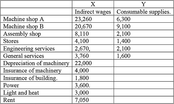
Note:
- Because of special fire risks, machine shop A is responsible for a special loading of insurance on the building. This results in a total building insurance cost for machine shop A as one third of the annual premium.
- The general services department is located in a building owned by the company. It is valued at $6,000 and is charged into costs at a notional value of 8% per annum. The cost is additional to the rent and rates shown above.
- The value of issues of material to the production departments are in the same proportion as shown above for consumable supplies.
The following data is also available:
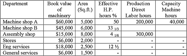
III. Ganesh Enterprises undertakes three different jobs A, B and C. All of them require the use of a special machine and also the use of a computer. The computer is hired and the hire charges work out to $420,000 per annum. The expenses regarding the machine are estimated as follows;
Rent for the quarter $ 17,500
Depreciation per annum $ 200,000
Indirect charges per annum $ 150,000
During the first month of operation, the following details were taken from the job register:
Number of hours the machine was used: A B C
i) Without the use of Computer 600 900 –
ii) With the use of the computer 400 600 1,000
Here, we have to compute the machine hour rate:-
- For the firm as a whole for the month when the computer was used and when the computer was not used.
- For the individual jobs A, B and C.
B3 Labor allocation
Labor cost incurred by a company is divided into two categories based on variability and controllability:
- Direct labor and indirect labor cost
- Controllable and non-controllable labor cost.
Direct labor cost is that portion of wages or salaries which can be identified with and charged to a single costing unit. Labor cost will be classified as direct cost when;
- There is a direct relationship between labor cost and the product or process or cost unit,
- Labor cost may be measured in the light of this relationship,
- Labor cost is sufficiently material in amount.
Indirect labor costs are those costs which are not identifiable in the production of specific goods or services. These labor costs are commonly used for production activities. Indirect labor cost consists of labor costs in service departments such as purchasing, engineering and time-keeping. Labor cost of certain workers in the production departments will also come in the category of indirect labor cost (foremen, material expediters and clerical assistants). Direct labor cost forms a part of the prime cost and indirect labor cost becomes a part of the overhead.
The importance of distinction between direct and indirect labor are as follows:
- Determination of accurate product cost
- Measurement of efficiency
- Preparation of informative labor cost analysis, avoiding serious errors in overhead allocation.
Controllable and non-controllable labor cost – these terms are often used in budgeting and variance analysis to describe costs that are either controllable or non-controllable with reference to a particular department. These terms are also used within particular time periods to reflect whether costs are controllable in the short run or whether they will require long-term action. When standard costing system is in vogue, it is important to guide management activity towards controllable areas of responsibility (see Figure B3.1).

Methods of remuneration
B3.1 Time rate system
Under this system, the unit of measurement is ‘time’. This system disregards the ‘output’ of a worker. The wage rate of a worker may be determined in hourly, daily, weekly or monthly basis.
The time rate system is useful in the following circumstances:
- Units of output are not distinguishable and measurable
- Employees have little control over the quantity of output or there is no clear-cut relationship between effort and output
- Work delays are frequent and beyond the control of employees
- Quality of work is especially important
Earnings = Hours worked × Rate per hour
B3.2 Piece-rate schemes
Wage payments are made according to the quantity or volume produced, i.e., the payment is made by piece or time spent in completing a piece or a ‘unit’. Piece-rate systems are very useful in the following circumstances.
- Units of output are measurable
- A clear relationship exists between employee effort and quantity of output
- Standardized job, fewer break down and regular work
Different piece rate schemes are discussed mentioned here:
B3.2.1 Straight piece work
Earnings = No. of units produced × Rate per unit
Advantages:
- Workers are paid only for the work produced
- The workers are constantly interested in increasing output
- It is simple and provides a sound basis for introduction of standard costing system.
B3.2.2 Standard hour system of piece work
It is essentially the same as the straight piece work system. The only major difference between straight piece work and the standard hour plan is that, under the latter plan, the standards are expressed in time per unit of output rather than money.
• When production is in excess of standard performance:
Earnings = Actual hours worked × Hourly rate of pay + Hourly rate of pay (Standard hours produced – Actual hours worked).
• When production is below standard performance:
Earning = Hourly rate of pay × Actual time.
Illustration 10:
The base rate of the job is $0.625 per hour and the performance standard is 0.16 hour per piece. A day consists of 8 hours. What will be the earning for Mr. R and Mr. S if they produce 100 and 40 pieces in a day?
Solution:
The performance of Mr. R is above standard i.e., SH =100 × 0.16 = 16 hours, where as day is of 8 hours.
Earnings = Actual hours worked × Hourly rate of pay + Hourly rate of pay (Standard hours produced – Actual hours worked).
= 8 × $ 0.625 + 0.625 (16 – 8).
= $10.
The performance of Mr. S is below standard i.e., SH = 40 × 0.16 hrs. = 6.40 hours.
Earnings = 8 × 0.625 = $ 5.
B3.2.3 Differential piece work system
This system recognizes that higher reward should be given to more efficient workers. This can be classified as
- Taylor System
- Merrick System
Taylor differential rate system
Earnings = 80% of piece rate when below standard.
Earnings = 120% of piece rate when at or above standard.
Merrick differential system
It is not as harsh as the Taylor differential piece rate on workers of low efficiency. This method encourages trainees and developing workers.
| Up to 83.33% of efficiency | Normal piece rate applicable |
| Above 83.33 % but up to 100% | 10% above normal rate |
| Above 100 % | 20% above normal rate |
Both time rate system and piece work system have got some glaring deficiencies. These deficiencies are sought to be overcome by adopting schemes which are combination of time rate and piece work system.
B3.2.4 Gantt task and bonus system
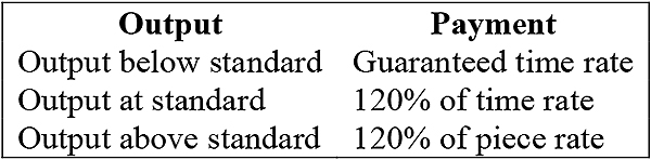
In this method labor cost is high for low production. It is specially recommended for application in heavy engineering and structural workshop, machine tool manufacturing industries, contract costing etc.
Illustration 11:
The performance of workers A, B and C in a factory in as follows:
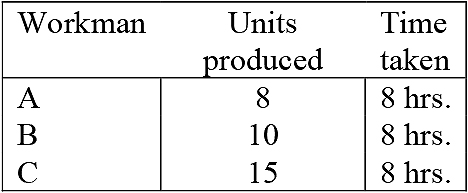
Standard production per day of 8 hours work is 10 units, day wage guaranteed $ 2 per hour, and bonus rate is 20%. We have to calculate wages of A, B and C under the Gantt Task Bonus Plan.
Solution:
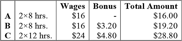
Time allowed for 15 units should be taken as 12 hours.
B3.2.5 Emerson’s efficiency system
Earning is calculated as follows:

B3.2.6 The Bedaux system
In this system, the standard time for a job is determined by time and motion studies. Allowed time for a job is stated in ‘points’. Under this system, a worker receives an hourly or a daily rate plus a bonus of 75% of the number of points saved multiplied by one-sixth of the hourly rate.
Earnings = Hours worked × Rate per hour + (0.75 × Rate per hour × Bedaux point saved/60).
Premium bonus plan guarantees the worker a minimum wage per hour but pays a premium for production in excess of the stipulated wages. Following schemes are under the Premium Bonus Plan:
Halsey plan
Earnings = Hours worked × Rate per hour + (Time saved × Rate per hour × 50/100).
Halsey-weir plan
Earnings = Hours worked × Rate per hour + (Time saved × Rate per hour × 33.33/100).
Rowan system
Earnings = Hours worked × Rate per hour + (Rate per hour × Hours worked × Time saved/ Time allowed).
Barth sharing plan
Earnings = Rate per hour × (Standard hours × Hours worked) ½
Scanlon plan
Earnings = Avg. annual salaries & wages × 100/Avg. annual salaries revenue.
Illustration 12:
Two employees, Mr. V and Mr. S, produce the same product using the same material and their normal wage rate is also the same. Mr. V is paid bonus according to the Rowan system, Mr. S is paid bonus according to the Hasley system. The time allowed to make the product is 100 hrs. Mr.V takes 60 hrs. while Mr.S takes 80 hrs. to complete the product. The factory overhead rate is $10 per man-hour actually worked. The factory cost for the product for Mr. V is $7,280 and Mr.S is $7,600.
We have to:
- Calculate the normal rate of wages
- Find the cost of materials
- Prepare a statement comparing the factory cost of products as made by the two employees
Solution:
Let x be the cost of material and y be the normal rate of wages per hour.
Factory cost of Mr. V.
Material cost = $x
Wages = 60y
Bonus under Rowan System,
= Hours worked × Rate per hour + (Rate per hour × Hours worked × Time saved/Time allowed).
= (y × 60 × 40/100) = 24y.
Overhead, 60 × 10 = 600
i.e., x + 84y = 7,280 – 600,
or, x + 84y = $6,680………………(I)
Factory cost of Mr. S.
Material cost = $x
Wages = 80 y
Bonus under Halsey System,
= Hrs. saved × Rate per hour × 50/100.
= 20 × ½ y = 10y.
Overhead, 80 × 10 = 800
i.e., x + 90y = 7,600 – 800,
or, x + 90y = $ 6,800………………(II)
From (I) & (II),
a) y = 20, i.e., Rate per hour = $ 20. (Normal wages)
b) Bonus paid to Mr. V = 24 × 20 = $480.
c) Bonus paid to Mr. S = 10 × 20 = $200.
d) The cost of material, x = 6680 – 84y = $ 5,000.
Comparative statement of the factory cost of the product made by two employees;

B3.3 Labor cost distribution
B3.3.1 Objectives
- Analyzing the labor times into direct and indirect labor by departments, jobs, work orders and processes
- Charging direct labor consisting of piece work, overtime and incentive bonus as production cost
- Treatment of indirect labor cost as overhead expenses.
B3.3.2 Idle time
Causes of idle time
- Production causes,
- – No power,
- – Machine breakdown,
- – Waiting for work
Administrative causes
- Economic causes
- – Seasonal,
- – Cyclical,
Industrial reasons
B3.3.3 Treatment of idle time
- Charge to factory overhead,
- Debit to the P & L account.
Overtime
Causes of overtime – scheduling more production and rush orders.
Overtime can be treated as follows:
- As a part of direct labor cost,
- As an element of manufacturing overhead, and
- Debiting directly to the P & L account.
B3.4 Case study
I. Garden Bore Ltd. manufactures various types of garden hose and operates a method of remuneration based on differential piece work. The output for each employee is expressed in standard units using the following conversion factors:
| Type of hose: | Rubber | Nylon | Plastic | ||
| Meters per standard unit | 100 | 70 | 130 |
The differential piece work rates are as follows:
| Weekly output per employee | Time allowed |
| First 180 units | 10 |
| 181- 300 units | 13 |
| All units over 300 units | 16 |
In addition an overtime premium is paid based on ‘time and one half’ with a basic week of 36 hours. The total minutes earned from the differential scheme are paid for at the time rate of $ 2.50 per hour. If piecework earnings are less than hours worked at e time rate then time earnings are paid. The following data relates to week 10:
We have to calculate the gross earnings for week 10 for each employee and also state why management and employees consider this remuneration method acceptable.
B4 Costing principles
Costing is the technique consisting of principles and rules, which govern the procedure of ascertaining the cost of products and services. Costing can be carried out by methods of integrated accounts, because it emphasizes the principles and rules.
The following are the techniques of costing used in industries for ascertaining the cost of products and services.
- Historical costing – Ascertaining costs after they have been incurred. This costing is based on recorded data and the costs arrived at are verifiable by past events.
- Standard costing – CIMA defines it as ‘a control technique which compares standard costs and revenues with actual results to obtain variances which are used to stimulate improved performance.’
- Marginal costing – It is the accounting system in which variable costs are charged to cost units and fixed costs of the period are written-off in full against the aggregate contribution. Its special value is in decision making.
- Direct costing – Under costing, a unit cost is assigned only the direct cost. All indirect costs are charged to the Profit and Loss account of the period in which they arise.
- Absorption costing – It is a technique that assigns all costs, i.e., both fixed and variable cost to product cost or cost of service rendered.
- Uniform costing – CIMA defines it as ‘the use by several undertakings of the same costing system, i.e., the same basic costing methods, principles and techniques.’
B4.1 Job costing
Job Costing helps to prepare estimates, monitor and control costs, compile bills, and measure the profitability of projects. It refers to the cost procedure or the system of cost accumulation that ascertains the costs of individual job or work order separately. A job represents the unit of costing. Job costing is used when products are dissimilar and non-repetitive in nature. A job may mean one unit of product or many units of identical/similar products covered by a single production order.
B4.1.1 Types of production activity suitable for job costing
- Production consists of special jobs or projects based on a customer’s specifications. Material contents and labor contents of each job are different. Each job uses the indirect facilities to a different extent.
- Production pattern is not repetitive and continuous.
- Virtually every job produced is somewhat different.
- Each job maintains its separate identity throughout the production stage.
- Different jobs are independent of each other.
B4.2 Routines under job costing
- Estimation: The production planning department or engineering department along with the cost accounting departments prepares the cost estimates that are based on bids prepared for prospective customers.
- Review of customer’s order by production planning department: The production planning department or engineering department analyzes the customer’s order. Based on its review and analysis, this department determines the material contents for the order and decides the schedule of the work to be done. For every review of a customer’s order, a production order is issued and each order is assigned a number called the job order number.
- Production order: A production order represents instructions to shop personnel to do work. It includes detailed instructions and drawings. A copy of it is sent to the accounting department (see Figure B4.1).

A sample production order
- Job order number: The production planning department assigns each production order a number, which is called job order number.
- Job Cost Card: The job sheet is designed to collect cost of materials, labor and factory overhead applicable to a specific job and is the most important document in job costing system (see Figure B4.2).
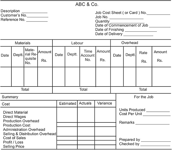
A sample job card
When a job is completed, the cost is totaled on the job cost sheet and is used as the basis for transferring the cost of a particular job order from work-in-process account to the finished goods account or the cost of sales account.
B4.2.1 Job costing module
Job Costing module tracks all costs related to a specific job or project. The Job Costing module provides management the information they need to quickly identify project costs which are out of line with budget estimates and requirements. Its flexible design makes it ideal for virtually any business that operates on a job or project basis. The Job Costing module breaks down jobs into as many phases and categories as required.
It supports unlimited cost types that can be grouped into six different classifications: labor, material, equipment, subcontractor, overhead, and miscellaneous. Each job can have an unlimited number of tasks or activities related to it. The job costing module retains original estimates to help budget more accurately, computes the percentage completed on each job, phase, and category to give up-to-the-minute job status.
Functions:
- Calculates billable amounts using either the percentage markup of cost or the unit price
- Allocates overhead on a per job basis, based on labor hours, labor dollars, material dollars or total job cost; can also record overhead directly to a phase
- Allocates employee benefits on a per-job basis, either as a percentage of labor dollars or as a flat rate per labor hour
- Uses job-related labor hours and costs, from Payroll or daily timecard or timesheet entries
- Saves job configurations as templates to simplify bidding and budgeting on subsequent jobs.
The Job Costing module monitors current jobs with budgeted and actual labor, material, and overhead rates which can be used in structuring new projects.
- It provides comparative information for appropriate pricing.
- The system allows interactive entry, editing, and posting. The work-in-process account is updated as costs are accumulated. Costs and inventory status are thereby reflected in the financial statements.
Reporting: The Job Costing module creates a variety of reports including a list of all or selected jobs, work-in-process journal, cost and budgetary reports etc. Presents key information by selected job, phase and category. Maintains detailed records on each job or periodically balances forward jobs selectively for summary records. Provides job information instantly with extensive on-screen inquiry functions.
Illustration 13:
Agrofed Ltd. receives an order to supply cattle feed to the farmers. The job passes through three departments, collecting costs as follows:

The job does not disrupt normal activity levels, which are as follows:
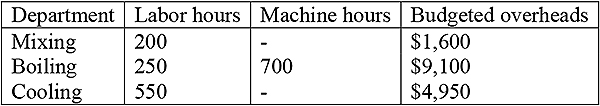
| Basis of absorption: | Mixing – Labor hours |
| Boiling – machine hours | |
| Cooling – Labor hours |
Selling and administrative expenses are 30% of factory cost.
We have to find out the profit/loss on this job, if the price agreed is $ 2,500.
Solution:

| *Overhead: | Mixing $ 1,600/200 = $8 per hour |
| Boiling $ 9,100/700 = $13 per hour | |
| Cooling $ 4,950/550 = $9 per labor hour. |
Batch Costing: Batch costing is essentially a variation of job costing. Instead of a single job, a number of similar product units are processed or manufactured in a group as a batch. Batch costing is used in following situations:
- Customer’s orders a quantity of identical items
- Internal manufacturing order is raised for a batch of identical parts, sub-assemblies or products to replenish stocks
- Where it is vital that color, or shading or specific characteristics of goods sold to customer is uniform
Batch costing is generally followed in toy making, footwear, biscuit factories, radio and watch manufacturing factories where manufacture of product or components can be done more conveniently in batches of different numbers.
Economic batch size: The size of a batch chosen for a production tem is likely to be a critical factor in achieving a least-cost operation. The economic batch size may be determined by using the Economic Production Batch Size (similar to EOQ) (see Figure B4.3).

Economic production batch size
Illustration 14:
Asian Paints Company has an annual demand from a single customer for 50,000 liters of a paint product. The total demand can be made up of a range of colors and will be produced in a continuous production run after which a set-up of the machinery will be required to accommodate the color change. The output of each shade of color will be stored and then delivered to the customer as a single load immediately before producing the next color. The costs are $100 per set-up (outsourced). The holding costs are incurred on rented storage space which costs $50 per sq. meter per annum. Each square meter can hold 250 liters, suitably stacked.
We have to :
- Calculate the total cost per year where batches may range from 4,000 to 10,000 liters in multiples of 1,000 liters and the production batch size which will minimize total cost.
- Calculate the batch size using the economic batch size formula for lowest total cost.
Solution:
a)
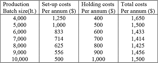
Note: For a production batch size of 5,000 liters,
No. of set-up per year = 50,000/5,000 = 10
Therefore, annual set-up cost per year = 100 × 10 = $ 1,000.
Average quantity in stock = 5,000/2 = 2,500 liters.
It assumes a constant rate of production. At the start of a batch, stock is zero. At the end, stock equals to the batch size.
Hence on average, 50% of the batch is on stock at any point of time.
b) Economic Production Batch Size = (2 × C2 × Q / C1 × T) 1/2
= (2 × 100 × 50,000/0.2 × 1) 1/2
= 7,071 liters
It is slightly different from the closest batch size (7,000 liters). In practice it is quite likely that a batch size which approximates to the minimum cost conditions will be chosen where a convenient quantity is used (7,000 liters) rather that the somewhat artificial quantity of 7,071 liters.
B4.3 Case studies
I. Amez Inc. manufactures special purpose industrial fans, which are sold at $400 per piece. The cost of sale is composed of 40% of direct material, 30% wages and 30% overhead. An increase in material price by 25% and in wage rate by 10% is expected in the forthcoming year; as a result of which the profit at current selling price may dwindle by 39% of present gross profit.
A statement showing current and future cost and profit at present selling price is required, along with the determining of the future selling price, if the present rate of gross profit is to be maintained.
B5 Process costing
Process Costing represents a type of cost procedure suitable for continuous and mass production industries producing homogeneous products. It is a cost accumulation system appropriate when products are manufactured through a continuous process. Each dept/cost center, prepares a cost of production report/ performance report.
Overview of process costing
Manufacturing costs are accumulated in processing departments in a process costing system. A processing department is any location in the organization where work is performed on a product and where materials, labor, and overhead costs are added to the product. Processing departments should also have two other features. First, the activity performed in the processing department should be essentially the same for all units that pass through the department. Second, the output of the department should be homogeneous. In process costing, the average cost of processing units for a period is assigned to each unit passing through the department.
Objectives
To determine how manufacturing costs be allocated to units completed, or to units started but not completed. Also to compute total unit costs for income determination.
B5.1 Features of process costing
- Costs accumulated by dept, or cost center
- Each dept has its own WIP A/C. – Debited: when costs incurred. Credited: when units complete/transferred to next dept
- Equivalent units (EU) are partially completed units restated in terms of completed units
- Unit costs determined by dept/cost center
- As units & costs leave each dept, the units & costs are carried over to the next dept; when units & costs leave the last dept, they can be used to determine the unit cost of finished goods
- If some units are spoiled in a process, the cost of the spoiled units is borne by units completed and closing stock of unfinished units at the end of the period
- Departmental cost of production reports/performance reports
Process costing is used in industries that produce basically homogenous products such as bricks, flour, and cement on a continuous basis.
There are some similarities between job-order and process costing systems:
- The same basic purpose exists in both systems in assigning material, labor, and overhead cost to products
- Both systems use the same basic manufacturing accounts: Manufacturing Overhead, Raw Materials, Work in Process, and Finished Goods
- The flow of costs through the manufacturing accounts is basically the same in both systems.
The differences between the job-order and process costing occur because the flow of units in a process costing system is more or less continuous and the units are essentially indistinguishable from one another. Under process costing:
- A single homogenous product is produced on a continuous basis over a long period of time. This differs from job-order costing in which many different products may be produced in a single period.
- Total costs are accumulated by the department, rather than by an individual job
- The department production report is the key document showing the accumulation and disposition of cost, (instead of the job-cost sheet)
The pattern of cost accumulations under process costing is illustrated through a flow chart in Figure B5.1.

Cost accumulations under process costing
B5.1.1 Basic steps for solution of problems in process Costing
Most process cost problems can be solved by a uniform approach involving the following steps:
Step No. 1 – Physical flow of production
It is to trace the physical flow of production. A statement is prepared showing input and output of the process in physical units.
It shows:
- Input in the form of opening inventory and fresh units
- Output in the form of:
- – Completed Opening WIP during process
- – Completed fresh units introduced
- – Closing WIP
Step No. 2 – The inventory costing method to be followed
The effect of using LIFO method, FIFO method and average method will be different on the unit cost of the process.
Step No. 3 – The state of introducing the material in process
Material can be introduced in the beginning, in the middle or at the end of the process. The stage at which material is introduced will significantly affect the cost per unit of the process.
Step No. 4 – work done on unfinished units should be expressed in terms of
‘equivalent production’
In order to calculate the average cost per unit, the total number of units must be determined. Partially completed units pose a difficulty that is overcome using the concept of equivalent units. Equivalent units are the equivalent, in terms of completed units, of partially completed units. The formula for computing equivalent units is:
Equivalent units = (Number of partially completed units × Percentage completion)
Equivalent units are the number of complete, whole units one could obtain from the materials and effort contained in partially completed units.
A company which had no beginning inventory completed 100 units last month. In addition, the company worked on another 60 units that were 40% complete. In terms of totally completed units, the amount of effort expended was equivalent to the production of 124 units ([100 + 60] × 40%).
Step No. 5 – Determining element-wise details of total cost of process to be
accounted for
This can be done by preparing a statement of cost for each element.
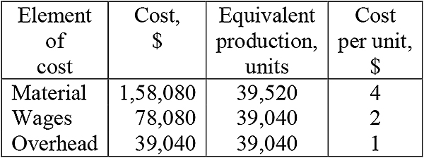
The element-wise details of cost should be collected and they should be divided by the number of equivalent units at cost per unit for each element.
Step No. 6 – Apportionment of process cost
This a statement prepared showing apportionment of process cost is as follows:
- Cost of units introduced and completed
- Cost of abnormal loss/ gain
- Cost of closing work-in-process.
Determination of cost of process with no process loss
All material, labor, direct expenses and proportionate share of overhead is considered as the raw material cost of that process.
Process costing with normal loss
Certain production techniques are of such a nature that some loss is inherent to the production. If the loss is within the specified limit, it is referred to as normal loss. The cost of normal loss in process is absorbed as additional cost by good production in the process. If the loss forms a particular percentage of production in the process, then the following equation is to be followed.
Production = (Opening Stock + units transferred in process – Closing Stock)
If the scrap fetches some value then the process cost per unit of the process is determined as follows;
Cost per unit = (Cost transferred to the process + additional cost in the process – Scrap value of units representing normal loss)/ (Unit in process – units scrapped.)
Process costing with abnormal loss
Abnormal loss refers to the loss which is not inherent to manufacturing operations. All cost relating to abnormal loss is debited to abnormal loss account and credited to process cost account so that the cost, (which could have been avoided according to norms of operations), is kept separately to facilitate control action to be taken. The following steps are suggested for valuation of abnormal loss in the process:
- Determine the normal production presuming no abnormal loss.
- Determine the total accumulated cost relating to the process, i.e., (Cost transferred to the process + additional cost in the process – Scrap value of units representing normal loss).
- Determine the cost per unit of normal production by dividing the result of step-b by result of step-a.
- Rate arrived at by step-c should be applied for valuation of both unit representing abnormal loss and output of the process.
Illustration 15:
2000 units are transferred to process B @ $4 per unit. Other cost details relating to this process are as follows:
| Material | $4,000 |
| Labor | $1,000 |
| Proportionate share of overhead for the process | $ 700 |
The normal loss has been estimated @ 10% of the process input. Units representing normal loss can be sold @ $1 per unit. Actual production in the process is 1700 units. We have to prepare process B account.
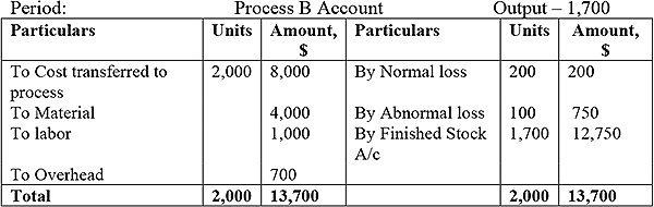
Notes:
- Normal loss is 10% of input, i.e. 2000 × 10/100 = 200 units
- If there had not been an abnormal loss, output of process b would have been 1800 units, i.e., Input – Normal loss
- Accumulated cost relating to the process
= Cost transferred + Material + Labor + overhead – Scrap value relating to normal loss.
= $ 8,000 + $ 4,000 + $ 1000 + $ 700 – $ 200 = $ 13,500. - Cost per unit of normal production = $13,500/1,800 units = $ 7.50.
- Abnormal loss of 100 units is valued at $ 7.50.
- Output 1,700 units should be valued at $ 7.50.
Process costing with abnormal gain
A reverse situation, where actual production may happen to be more than what the norms of the company permit, i.e., actual output is 95 units from a process with 10% normal loss. These 5 units represent abnormal gain of that process. The value of units relating to abnormal gain is debited to process account and credited to abnormal gain account. The following steps are suggested for valuation of abnormal gain in the process:
- Determine the normal production presuming no abnormal gain
- Determine the total accumulated cost relating to the process, i.e., (Cost transferred to the process + additional cost in the process – Scrap value of units representing normal loss)
- Determine the cost per unit of normal production by dividing the result of step-b by result of step-a
- Rate arrived at by step-c should be applied for valuation of both unit representing abnormal gain and output of the process transferred to either next process or finished stock account.
B5.2 Case studies
I. A product is finished in three stages I, II & III. At the first stage a quantity of 72,000 kg was delivered at a cost of $2.50 per kg. The entire material was consumed. The production particulars with the allocated expenses were indicated in the table below.

The producer has assessed the cost at $6.77 per kg based on input expenditure and the finished output. Estimated profit is $36,500 with a selling price at $7.50 per kg. Normal wastage is to be considered as 5% for each stage and no excess wastage is to be allowed to inflate the cost of the end product.
B6 Activity based costing
Activity based costing is not a distinct method of costing like job and process costing. It is only a new practice in the process of attribution of costs to jobs or processes. In the context of activity based costing, the costs are collected according to activities such as material ordering, handling, quality testing, machine setups, customer support service etc.
It is an accounting technique that allows an organization to determine the actual cost associated with each product and service produced by the organization without regard to the organizational structure.
B6.1 Activity-based costing system

Activity-based costing system
In order to achieve the major goals of business process improvement, process simplification and improvement, it is essential to fully understand the cost, time, and quality of activities performed by employees or machines throughout an entire organization. ABC methods enable managers to cost out measurements to business simplification and process improvement (see Figure B6.1).
Activity Based Costing is a modeling technique where costs are expressed in terms of Resources, Activities, and Products. Work (activities) is performed to create products, and resources are consumed by the work.
B6.2 Basic elements of ABC
- Resources
- Activities
- Cost Objects
- Resource Drivers
- Activity Drivers (see Figure B6.2)

ABC model
Reasons for the introduction of ABC
- Traditional costing is based on assumption: Relation between overhead and the volume based measure
- It often fails to highlight inter-relationship among activities in different departments
- Arbitrarily allocates overhead to the cost objects
- Total company’s overhead is allocated to the products based on volume based measure e.g. labor hours, machine hours
- Traditional costing which is based on averages and estimation
- To determine the ‘true’ cost for a cost object (product, job, service, or customer).
In any business the ‘true’ cost of a product is important
- To identify money makers/money losers
- To finding an economic break-even point
- To compare different options
- To discover opportunities for cost improvement
- To prepare and actualize a business plan
- To improve strategic decision making
Basics of activity based costing
- Identify the major activities such as material handling, mechanical insertion of parts, manual insertion of parts, wave soldering, quality testing etc
- Determine the ‘cost drivers’ for each activity. The cost driver is the underlying factor(s) which causes the incurrence of cost relating to that activity. Cost drivers link activities and resource-consumption and thereby generate less arbitrary costs for decision making
- Create cost pools to collect activity costs having the same cost driver
- Attribute the cost of activities in the cost pools to products/services based on the cost drivers
Illustration 16:

Figure B6.3
Two types of cost drivers–resource drivers and activity drivers (see Figure B6.3)
- Resource drivers assign resource costs to activities based upon consumption
- Activity drivers indicate consumption of activities by cost objects
Five activities that need to occur in order to determine activity costs
- Identify activities
- Determine cost for each activity
- Determine cost drivers
- Collect activity data
- Calculate product cost
Illustration 17:
Traditional costing
In a company two products: product A and product B

Total overhead: $ 100,000.00
Total direct labor: 2,000 hours
$ 100,000/2000 hours = $ 50 / hour
Product A: 1 hour of direct labor
Product B: 2 hours of direct labor
B6.3 Activity based costing
Step-1: Identify activities
Set-up
Machining
Receiving
Packing
Engineering
Step-2: Determine cost for each activity
| Set-up | $10,000 |
| Machining | $40,000 |
| Receiving | $10,000 |
| Packing | $10,000 |
| Engineering | $30,000 |
Step-3: Determine cost drivers
Number of Setups
Machining Hours
Number of Receipts
Number of Deliveries
Engineering Hours
Step-4: Activity data

Step-5: Product cost calculation
Overhead for Product A: $24,500: 100 = $245
Overhead for Product B: $75,500: 950 = $79.47
Traditional costing (TC) vs. ABC

ABC example
ABC is a powerful tool for measuring business performance, determining the cost of business process outputs, and is used as a means of identifying opportunities to improve business process effectiveness and efficiency. Below is a process diagram with the sub-activities shown in a sequential activity order for Correspondence process, which comes under the Executive Secretariat in the Office of the Administrator. For the ABC, the sub-activities were then analyzed and a cost derived (see Figure B6.4).

A process diagram
Disadvantages of ABC
- It is essentially not the panacea for all ills
- It absorbs a lot of resources
- Too much emphasis on customer viability can lead to problems such as cheaper products and, therefore, potentially lower sales
- It may lead to weaker customer segmentation
- It takes no account of opportunity cost.
B7 Backflush costing
This is introduced in February 1991, focuses on output and then works back to apply manufacturing costs to units sold and to inventories. It is an accounting system that applies costs to products only when production is complete. Blackflush costing attempts to remove non-value-added activities from costing systems, i.e., the cost of tracking work-in-process exceeds the benefits for many companies. Material inventory of work-in-process is typically small compared to the costs of goods produced and sold.
B7.1 Overview of journal entry trigger points
Trigger point = Point where journal entries are made that accumulate production costs related to the units.
1st variation: Two trigger points = Purchase of raw materials and finished goods completed (RIP and F/G accts- no w/p account).
2nd variation: Two trigger points = Purchase of raw materials and finished units sold (one inventory acct- no W/P or F/G accounts).
3rd variation: One trigger point = Finished goods completion (one F/G account-no RIP or W/P accounts).
B7.2 Difficulties of backflush costing
- It does not strictly adhere to generally accepted accounting principles of external reporting.
- Absence of audit trials.
- It does not identify the use of resources at each step of the production process.
- Backflush Costing is suitable only for JIT production system with virtually no direct material inventory and minimum WIP inventories.
B8 Lifecycle costing
For understanding lifecycle costing, it is necessary to understand product life cycle. The product life cycle starts from the time of initial research and development to the time, at which sales and support to customers are withdrawn. Lifecycle costing tracks and accumulates the actual cost attributable to each product from its initial research and development to its final resourcing and support in the market place. It focuses on total costs (capital cost + revenue cost) over the products life including design and development, acquisition, operation, maintenance and servicing. CIMA defines lifecycle costing ‘as the practice of obtaining over their life-times, the best use of physical assets at the lowest cost to the entity.’ It is achieved through a combination of management, financial, engineering and other disciplines. Life cycle costing emphasis to relate the total life cycle costs to identifiable units of performance to arrive at the optimum decision.
Example:
We want to compare the cost of different power supply options such as photovoltaic, fueled generators, or extended utility power lines. The initial costs of these options will be different as will the costs of operation, maintenance, and repair or replacement. An LCC analysis can help compare the power supply options. The LCC analysis consists of finding the present worth of any expense expected to occur over the reasonable life of the system. To be included in the LCC analysis, any item must be assigned a cost, even though there are considerations to which a monetary value is not easily attached. For instance, the cost of a gallon of diesel fuel may be known, the cost of storing the fuel at the site may be estimated with reasonable confidence, but, the cost of pollution caused by the generator may require an educated guess. Also, the competing power systems will differ in performance and reliability. To obtain a good comparison, the reliability and performance must be the same. This can be done by upgrading the design of the least reliable system to match the power availability of the best. In some cases, we may have to include the cost of redundant components to make the reliability of the two systems equal. For instance, if it takes one month to completely rebuild a diesel generator, we should include the cost of a replacement unit in the LCC calculation. A meaningful LCC comparison can only be made if each system can perform the same work with the same reliability.
B8.1 LCC calculation
The lifecycle cost of a project can be calculated using the formula:
LCC = C + Mpw + E pw + R pw – S pw.
The pw subscript indicates the present worth of each factor. The capital cost (C) of a project includes the initial capital expense for equipment, the system design, engineering, and installation. This cost is always considered as a single payment occurring in the initial year of the project, regardless of how the project is financed.
Maintenance (M) is the sum of all yearly scheduled operation and maintenance (O&M) costs. Fuel or equipment replacement costs are not included. O&M costs include such items as an operator’s salary, inspections, insurance, property tax, and all scheduled maintenance.
The energy cost (E) of a system is the sum of the yearly fuel cost. Energy cost is calculated separately from operation and maintenance costs, so that differential fuel inflation rates may be used.
Replacement cost (R) is the sum of all repair and equipment replacement cost anticipated over the life of the system. The replacement of a battery is a good example of such a cost that may occur once or twice during the life of a PV system. Normally, these costs occur in specific years and the entire cost is included in those years.
The salvage value (S) of a system is its net worth in the final year of the lifecycle period. It is common practice to assign a salvage value of 20 percent of original cost for mechanical equipment that can be moved. This rate can be modified depending on other factors such as obsolescence and condition of equipment.
B8.2 Advantages of lifecycle costing
- It can provide important information for pricing decisions. This is essential in present day context because for some products, development period is relatively long and many costs are incurred prior and after manufacturing.
- It helps the manager develop insight and plan so that it is possible to generate revenue from the product.
- It broadens the perspective of managers because the complete lifecycle relating to a product is kept in view and for this reason the terms ‘cradle to grave’ and ‘womb to tomb’ are often used in the context of life-costing. It does not have a calendar based focus, but considers the whole life span of the product.
- Full costs associated with each product become relatively more visible. Manufacturing costs are highly visible in most accounting systems. However the costs associated with upstream areas (e.g. R & D) and downstream areas (e.g. customer service) are often less visible at a product-by-product level in the organization following traditional costing. Lifecycle costing finds solution to this problem.
- Lifecycle costing highlights inter-relationships across cost categories. Many companies, who cut R & D costs, later experience major increases in customer-service related costs in subsequent years. The products of these companies also fail to meet promised quality performance levels. A lifecycle revenue and costs statement highlights hidden areas, which get obscured in cost statements having a calendar based focus.
- It is immensely useful in capital budgeting decisions (i.e., long term decision making).It makes explicit the trade-off between higher capital costs and lower maintenance running costs.
B9 Marginal costing
CIMA defines marginal costing as ‘the cost of one unit of product or service which would be avoided if that unit were not produced or provided.’ Marginal costing is not a distinct method of costing like job costing or process costing. It is a technique which provides presentation of cost data in such a way that a true cost-volume-profit relationship is revealed. It is an accounting system in which variable cost is charged to the cost units and fixed costs of the period are written-off in full against the aggregate contribution. Its special value is in decision-making. It is presumed that costs can be divided in two categories, i.e., fixed and variable cost.
B9.1 Process of marginal costing
Under marginal costing, the difference between sales and marginal cost of sales is found out. This difference is technically called contribution. Contribution provides for fixed cost and profit. Excess of contribution over fixed cost is profit or net margin. Emphasis remains on increasing total contribution.
B9.2 Break-even point
Break-even point is the point of sale at which a company makes neither profit nor loss. The marginal costing technique is based on the idea that difference of sales and variable cost of sales provides for a fund, which is referred to as contribution. At break-even point, the contribution is just enough to provide for fixed cost. If actual sales level is above break-even point, the company will make profit. If an actual sale is below break-even point the company will incur loss. When cost-volume-profit relationship is presented graphically, the point, at which total cost line and total sales line intersect each other will be the break-even point (see Figure B9.1).

Break-even point
B9.2.1 Basic marginal cost equation
We know that: Sales – Cost = Profit,
Or, Sales – Variable costs = Fixed costs + Profit
It is known as marginal equation and is expressed as follows:
S – V = F + P,
Profit/volume ratio
When the contribution from sales is expressed as a percentage of sales value, it is known as profit/volume ratio. Better P/V ratio is an index of sound ‘financial health’ of a company. It is expressed as:
| P/V ratio | = (Sales – Marginal cost of sales)/Sales |
| = Change in contribution/ change in sales | |
| = Change in profit/ change in sales. |
Advantages of P/V ratio
- It helps in determining the break-even point
- It helps in determining profit at various sales levels
- It is to find out the sales volume to earn a desired quantum of profit
- It determines relative profitability of different products, processes and departments.
Improvement of P/V ratio
P/V ratio can be improved by improving the contribution. Contribution can be improved by any of the following steps:
- Increase in the sale price
- Reducing marginal cost by efficient utilization of men, materials and machines
- Concentrating on the sale of products with relatively better P/V ratio.
Illustration 18:
PRF & Co. produces a single article. Following cost data is given about its product:-
| Selling price per unit | $ 20 |
| Marginal Cost per unit | $ 12 |
| Fixed cost per annum | $ 800 |
We have to calculate:
- P/V Ratio,
- Break-even sales,
- Sales to earn profit of $ 1,000
- Profit at sales of $ 6,000
- New break-even sales, if sales price is reduced by 10%.
Solution
Sales – Variable costs = Fixed costs + Profit
By multiplying and dividing left hand side by S,
S(S-V)/S = F + P,
Or, S X P/V Ratio = Contribution
- P/V Ratio = Contribution / Sales
= (20 – 12)/20 × 100 = 8/20 × 100 = 40%.
- Break-even sales,
S X P/V Ratio = Fixed Cost
(At break-even sales, contribution is equal to fixed cost)
By putting the values: S × 40/100 = 800, S = $2,000 or 100 units.
- The sales to earn a profit of $ 1,000
S × P/V Ratio = F + P,
By putting the values:
S × 40/100 = 800 + 1,000, S = $4,500 or 225 units.
- Profit at sales of $ 6,000,
S × P/V Ratio = F + P,
By putting the values:
$6,000 × 40/100 = $800 + P,
P = $ 1,600.
- New break-even sales, if sales price is reduced by 10%.
New Sales Price = $20 – $2 = $18
Marginal cost = $12
Contribution = $6
P/V Ratio = 6/18 × 100, or 33.33%
S × P/V ratio = F (at BEP contribution is equal to fixed cost)
S × 100/300 = $800,
S = $ 2,400.
Cost-volume-profit relationship
Profit is actually the result of interplay of different factors like cost, volume and selling price. The conventional income and expenditure statement does not provide any answer to the following basic questions:
- What should be the volume to be attempted for obtaining a desired profit?
- How will the change in selling price affect the profit position of the company?
- How will the change in cost affect profit?
- What should be the optimum mix of the company?
The answer to all these questions is provided by cost-volume-profit analysis.
Cost-volume-profit relationship
The result of analysis of Cost-Volume-Profit Relationship can be presented by the following statement.
Forecast of Cost-Volume-Profit Analysis at Different Activity Levels

Illustration 18:
ABC Ltd. is considering renting additional factory space to make two products, L-1 & L-2. Company’s monthly budget is as follows:

The fixed overheads in the budget can only be avoided if neither product is manufactured. Facilities are fully interchangeable between products.
As an alternative to the manual production process assumed in the budget, the company has the option of adopting a computer-aided process. This process would cut variable costs of production by 15% and increase fixed costs by $12,000 per month.
The management is confident about the cost forecasts, but there is considerable uncertainty over demand for the new products. The management believes the company will have to depart from its usual cash sales policy in order to sell L-2. An average of three months credit would be given and bad-debts and administration costs would probably amount to 4% of sales revenue for this product. Both the products will be sold at the price assumed in the budget. The company has a cost of capital of 2% per month. No stocks will be held.
We have to calculate:
- The sales revenue at which operations will break-even for each process (manual and computer-aided) and the sales revenues at which ABC Ltd. will be indifferent between the two processes.
If L-1 alone is sold;
If L-1 & L-2 units are sold in the ratio 4:1, with L-2 being sold on credit
- We need to explain the implications of our results with regard to the financial viability of L-1 and L-2.
Solution:
Manual Production Computer Aided
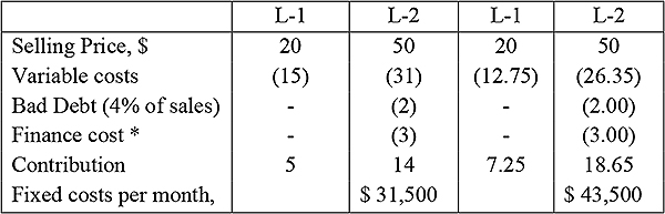
* Finance cost = $50 × 0.02 × 3 months = $3.00
i) Only L-1 is sold
Manual process break-even point = 31,500 / 5 = 6,300 units
Or, = 6,300 × $ 20 = $126,000
Computer Aided break-even point =43,500 / 7.25 = 6,000 units
Or, = 6,000 × $ 20 = $ 120,000
The point of indifference here will be the point of sales at which contribution under the two alternatives is the same.
Suppose indifference point = n units
5n + 31,500 = 7.25n + 43,500
So, n = 5,333 units = 5,333 × $ 20 = $10,667.
Sales of L-1 and L-2 in the ratio of 4:1,
Manual Process:
Average contribution = {(4 × 5) + (1 × 14)}/5 = $6.80
Break-even point = $31,500/6.80 = 4632.35 units
Or, 4632.35 × $26# = $ 120,441
Note:
- Break-even point (sales revenue) = Break-even point in unit × Average selling price per unit.
- Average sales revenue per unit = {(4 × 20) + (1 × 50)}/5 = $26#
If L-1 alone is sold, budgeted sales are 4,000 units and break-even sales are 6,000 units (Computer aided process) and 6,300 units (Manual process).Therefore, there is little point producing L-1 on its own. Even if the two products are substitutes, total budgeted sales are 6,000 units and L-1 is still not worth selling on its own. Only if sales are limited to $180,000 (total budgeted sales revenue) L-1 will be worth selling on its own. However, the presumption that products are perfect substitutes and $180,000 sales can be generated is likely to be over-optimistic. In other words, a single-product policy is very risky. Launching both-products policy is a profitable alternative. It is better to sell L-2 in preference to L-1 based on margin of safety. It is 1375 units of L-1 (34%) and 688 units of L-2 (34%). It is recommended that both the products be sold and computer aided process be adapted.
B9.3 Case study
I. A person is planning to give up his job as an engineer, with a current salary of $1400 per month, and go into business on his own, assembling a component which he has invented. He can obtain the parts required from various manufactures. The sales potential of the component has been estimated by some research are as follows;
- Between 600 and 900 units per month if the price is $ 25 per unit
- Between 900 and 1,250 units per month if the price is $ 22 per unit.
The cost of parts required would be $14 per completed component. However, if more than 1,000 units can be sold each month, a discount of 5% would be received from the parts’ suppliers on all purchases. Assembly cost would be $6,000 per month for assembly of up to 750 components. Beyond this level of activity, costs would increase to $7,000 per month. He has already spent $3,000 on development, which he would write off over the first five years of the venture on a straight line basis.
Calculate for each of the possible sales levels whether that person could expect to benefit by going into business on his own. Also calculate the break-even point of the venture for each of the selling prices.
II. XYZ Inc. manufactures four products, namely A, B, C and D, using the same plant and process. The following information relates to a production period:
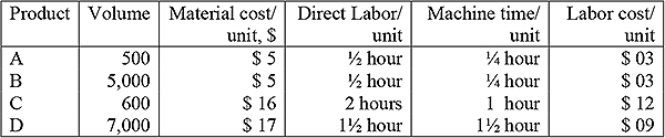
Factory overhead applicable to machine-oriented activity is $37,424.
Set-up costs are $4,355.
The cost of ordering material is $1,920 and material handling is $7,580.
Administration for spare parts $8,600.These overhead costs are absorbed by products on a machine hour rate of $4.8 per hour, giving an overhead cost per product of:

However, investigation into the production overhead activities for the period reveals the following total:

It is required
- To compute an overhead cost per product using activity based costing, tracing overheads to production units by means of cost drivers
- To comment briefly on the differences disclosed between overheads traced by the present system and those traced by activity based costing.
B10 Cost estimation
B10.1 What is cost estimation?
Cost estimating is one of the fundamental and yet most challenging tasks for contract and project managers. The Society of Cost Estimating and Analysis provides the following definition of cost estimating: ‘The art of approximating the probable cost or value of something based on information available at the time.’
Estimates of the costs associated with project /manufacturing tasks are made for many reasons. For example to:
- Justify planned capital expenditure
- Determine likely production costs, for new or modified products
- Focus attention on areas of high cost
In principal, estimates are made of the resources required (e.g. materials, labor and equipment), the cost of those resources and the time for which they will be used. From these factors an estimate of the costs of carrying out a manufacturing process is made.
B10.2 Cost estimating process
The cost estimating process can be viewed as a systematic approach consisting of the following steps:
- Plan the estimate
- Research, collect, and analyze data
- Develop estimate structure
- Determine estimating methodologies
- Compute the cost estimate
- Document and present the estimate to decision makers for use
The purpose of estimating
- Quoting, bidding, or evaluating bids
- Profitability analysis
- Basis for make versus buy decisions
- Investment justification
- Basis for comparing manufacturing methods
- Basis for cost reduction
- Planning new products and services;
B10.2.1 Cost estimation plan
The first step in developing an estimate is defining the estimating task and planning the work to be accomplished. The definition and planning stage includes determining the ultimate use of the estimate, understanding the level of detail required, outlining the total characterization of the system being estimated, establishing ground rules and assumptions, selecting the estimating methodologies, and finally, summarizing all of these in an estimating plan. The task definition and planning is an integral part of any estimate and represents the initial work effort and provides the framework for achieving a competent estimate efficiently. The purpose of the estimate is determined by its ultimate use, which in turn will influence the level of detail required and the scope it encompasses.
Scope of the estimate
The scope provides boundaries for the development of an estimate. It describes the breadth of the analysis and provides a time frame for accomplishment. Several factors drive the scope of the estimate:
- The elements that the recipient of the estimate wants included
- Criticality of the estimate
- Resources available
- Point at which the program is in acquisition
It is important that all stakeholders agree to the scope of an estimate, in order to avoid major changes once the analysis has begun. In addition, the cost estimator must have a full understanding of the scope prior to the analysis and should keep the scope in mind during the conduct of the analysis. The scope provides a focus for the estimator as the analysis progresses.
Knowing the general ‘character’ of the project provides the estimator with a good understanding of what is being estimated. The character of the project refers to those characteristics that distinguish it from other projects. Some of these characteristics include:
- Purpose or mission,
- Physical characteristics,
- Performance characteristics,
- Maintenance concept, and
- Identification of similar projects.
After learning how the estimate is to be used, the level of detail required, and the character of the project being estimated, the estimator is in a better position to establish major ground rules and assumptions (i.e., the conditions upon which an estimate will be based). Ground rules usually are considered directive in nature and the estimator has no choice but to use them. In the absence of firm ground rules, assumptions must be made regarding key conditions which may impact the cost estimate results. The project schedule, if one exists, is an example of a ground rule. If a schedule does not exist, the estimator must assume one.
Selecting the estimating methodologies to be employed is probably the most difficult part of planning the estimate since methodology selection is dependent on data availability. Therefore, the estimating methodologies selected during this planning stage may have to be modified or even changed completely later on if the available data do not support the selected technique. It is still helpful, however, to specify desired estimating methods because doing so provides the estimator with a starting point.
It is important to understand that task definition and planning is an integral part of any estimate. It represents the beginning work effort and sets the stage for achieving a competent estimate efficiently.
B10.2.2 Research, collect, and analyze data
During the data research and analysis step, the estimator fine-tunes his estimating plan. Planned methodologies may, turn out to be unusable due to lack of data. New methodologies may have to be developed or new models acquired. Cost research may reveal better methodologies or analogies than those identified in the original plan. During this step, also, the estimator normalizes the data so that it is useable for the estimate.
During the process of data research, collection, and analysis, the estimating team should adopt a disciplined approach to data management. The key to data research is to narrow the focus in order to achieve a viable database in the time available to collect and analyze it. Data collection should be organized, systematic, and well documented to permit easy updating. The objective of data analysis is to ensure that the data collected are applicable to the estimating task at hand and to normalize the data for proper application.
B10.2.3 Develop estimate structure
An essential ingredient for any successful estimate is the work breakdown structure (WBS) since it provides the overall framework for the estimate. The estimator must decide at which level in the WBS to construct the estimate. This will affect the amount of detail in the estimate and have an impact on choice of estimating methodology. For instance, if the system being procured can be defined in great detail, there will be numerous levels in the WBS and estimating methodologies can be chosen at a low level of detail. Reviewing the work element levels should help put the estimate in perspective and the typical element levels are shown here

B10.2.4 Determine estimating methodologies
Estimating is a forecast of future costs based on a logical extrapolation of data currently available. Again, data availability is a key consideration in selecting the estimating methodology. In fact, the amount and quality of data available often dictate the estimating approach. Common estimating methodologies are identified and defined in Figure B10.1.

Estimating methodology
B10.2.5 Putting the estimate together and crunching the numbers
At this stage of the process, the estimators put it all together and crunch the numbers. Many pieces of the estimate have been collected. These pieces need to be assembled into a whole – the final estimate. This section addresses the steps that estimators should go through to load the estimate into the automated tool they have chosen for the estimate. The use of automated tools greatly simplifies updating, documenting, and calculation of the estimate.
The steps addressed are:
- Entering data and methodologies into the physical structure of the estimate (the WBS)
- Time phasing the estimate
- Dealing with inflation.
Entering data and methodologies into the physical structure of the estimate
A computer program is essential to the task of assembling the estimate. Programs allow efficient processing of data, electronic calculations, easier documentation, and simpler updating. There are myriad software tools available to facilitate this process. The most commonly used and widely available program, however, is the electronic spreadsheet. The WBS is the structure of the estimate. The first step is to enter the WBS into the computer program. Next, estimating methodologies are entered directly into the spreadsheet, or the spreadsheet takes an input from a separate model.
Time phasing the estimate
Estimates reflect tasks that occur over time. Obviously, cost estimates will vary with the time period (in which the work occurs), due to changes in labor rates and other factors. Say, the number of man-hours needed to complete a software development effort may be higher if the development time is shortened, or lower if it is lengthened. Time phasing is essential in order to determine resource requirements, apply inflation factors, and arrange for resource availability. Determining resource requirements is an important program management task. The program manager must also ensure that money will be available to pay for the people and the materials at the time they are needed. The first step to doing this successfully is the scheduling step. The estimator estimates inflation for the future by using projected inflation rates and time phases the rates over the period of performance of the task. This will let the program manager know how much a task will cost in the dollars relevant at a future time. This is essential for preparing a realistic budget.
Dealing with inflation
One of the primary purposes for time phasing estimates is that they may be expressed in current dollars and included in budget requests. It is the process of translating base year estimates into ‘other year’ dollars through the application of index numbers.
B10.2.6 Document the cost estimation
The requirement to develop the cost estimate document in a manner that allows an independent cost estimator to understand the methodology adequately to reconstruct the estimate in detail is the keystone to high quality cost estimate documentation.
Documentation content
The cost estimator should understand that every estimate will not be documented to this level of detail. Documentation must be tailored to align with the size and visibility of the program estimates. Consequently, when documenting smaller programs or projects, this tailoring provision would be employed to downscope the content structure provided below. Specifics of this downscoping would be dictated by the size and nature of the program or project involved. However, the requirement for enough detail to support replication must be sustained by the tailored documentation.
Introduction
This portion of the cost estimate document will provide the reader a thumbnail sketch of the program estimated, who estimated it, how it was estimated, and the data used in developing the estimate. The introduction is a highly valuable overview for managers and an extremely useful reference for estimators attempting to determine the applicability of the document’s main body to a current estimate or research study.
The introduction should address the following areas:
- Purpose of the Estimate – State why the estimate was done, whether it is an initial or updated prior estimate and, if an update, identify the prior estimate.
- Direction – Identify the requesting organization, briefly state the specific tasking, and cite relevant correspondence. Copies of tasking messages can be included here, in the main body, or as an appendix to the documentation package.
- Team Composition – Identify each team member, his or her organization, and area of responsibility.
- Program Background and System Description – Characterize significant program and system aspects and status in terms of work accomplished to date, current position, and work remaining. Include information such as detailed technical and programmatic descriptions, pictures of the system and major components, performance parameters, support concepts, contract types, acquisition strategies, and other information that will assist the document user in fully understanding the system estimated.
- Scope of the Estimate – Describe acquisition phases, appropriations, and time periods encompassed by the estimate. Further, if specific areas were not addressed by the estimate, state the reason.
- Program Schedule – Include the master schedule for development, production, and deployment, as well as a detailed delivery schedule.
- Ground Rules and Assumptions – List all technical and programmatic conditions that formed the basis for the estimate.
- Inflation Rates – Simply state which set of inflation rates were used for the basic estimate. A detailed table portraying the rates used can be included either in the main body or as an appendix to the documentation package.
- Estimate Summary – Identify the primary methodology and techniques that were employed to construct the estimate, along with a general statement that relates the rationale for having selected these particular methodologies and techniques. Also, briefly describe the actual cost data and its sources that were used to develop or verify the estimate. The final portion of this section should portray estimate results by major cost elements, in both constant year and current year dollars. A bottom-line track to the previous estimate also should be included, if applicable. For each major cost element, a page reference to the main body of the documentation where a complete description of its estimate can be located should be included.
- Main Body Overview – Provide an overview of how the document’s main body is organized and describe any of its aspects that may facilitate its use.
Main body
This portion of the documentation should describe the derivation of the cost estimate in sufficient detail to allow a cost estimator, independent of the original estimating team, to replicate the estimate. Developing this portion of the document properly requires that documentation be written in parallel with developing the estimate. The main body should be divided into sections using the content areas and titles shown below. Following these guidelines, pertaining to the document’s main body content structure, will allow the estimating team to develop a comprehensive document efficiently.
Estimate description
This provides a detailed description of the primary methods, techniques, and data used to generate each element of the estimate.
- Data – Show all data used, its source (e.g., actuals on current contract/analogous program), and normalization procedure.
- Labor Rates – Identify direct and indirect labor rates as industrial averages or contractor specific, their content, and how they were developed.
- Labor Hours – Discuss how functional labor hours were developed (e.g., contractor proposal, build-up from analogous program, engineering assessments).
- Material/Subcontracts – Depict the material, purchased parts, and subcontracted items that are required, and the development of their cost (e.g., vendor quotes, negotiated subcontracts, catalog prices).
- Cost Improvement Curves – Include the method used to describe the curve selected in terms of its slope, source, and relevance to the cost element and program being estimated. Any unique aspects of curve application must be included in this section.
- Factors and Cost Estimating Relationships (CERs) – Provide the basis, development, and/or source of all factors and CERs used for areas such as support equipment, data, training, etc. This discussion must include a description of how the factor was applied (e.g., against recurring manufacturing labor costs) and its relevance to the program being estimated.
- Cost Models – Describe all models used and their relevance to the estimate, along with complete details regarding parametric input and output (include detailed runs here or as an appendix to the documentation package) and any calibration performed to ensure the model served as an appropriate estimating tool for the cost element and program involved.
- Inflation Index – Document the specific indices and computations used in the estimate including those employed to normalize historical data. A detailed table portraying the rates used can be included either here or as an appendix to the documentation package.
- Timephasing – Identify/describe the approach used to phase the estimate.
- Sufficiency Reviews and Acceptance – Discuss the process used for reviewing an existing cost element estimate to determine its sufficiency and acceptability for incorporation into the estimate. This process should be applied to existing government and contractor estimates that are accepted as throughput to the estimate.
- Estimator Judgment – Document the logic and rationale that led to specific conclusions reached by the estimator regarding various aspects of the estimate.
- Risk and Confidence – Show the details of all risk analysis conducted and how it formed the basis for reaching conclusions regarding estimate confidence.
Documentation format
Documentation must be organized logically with clearly titled, easy to follow sections. The following considerations will contribute towards achieving high quality, useable cost estimate documentation:
- The documentation package should include the program name, reason for the estimate, the identity of both the tasking organization (and office symbol) as well as the organization that accomplished the estimate, and the ‘as of’ date.
- A table of contents should be included that identifies the titles of each numbered section and subsection along with page numbers.
- Pages should be numbered either sequentially or sequentially within each section.
- Where the same data or method is used repeatedly, it should be described in detail at the point of original use, and referenced by page number thereafter.
- All terms and acronyms should be defined fully at the point of first use.
- All figures and tables should be identified by numbers and clear descriptive titles.
- Cross-references should be used to assist the reader in understanding where areas addressing the same subject are located in the document.
- The first time documented information is used, its source should be cited and added to the reference list contained at the end of the documentation package. When the same source is used thereafter, only the reference number needs to be cited.
Documentation process
To carry out the documentation process effectively, the team leader should develop an outline. This estimate specific outline will provide a road map that depicts to the team the planned structure and content of the final documentation package. With this blueprint and the documentation requirements established in this chapter, the estimator can develop notes that will form the basis for the estimate’s documentation. If accomplished properly, the time to clean up and refine the estimator’s notes into final documentation form will be minimized.
A flow diagram (see Figure B10.2) of the documentation process is given below.
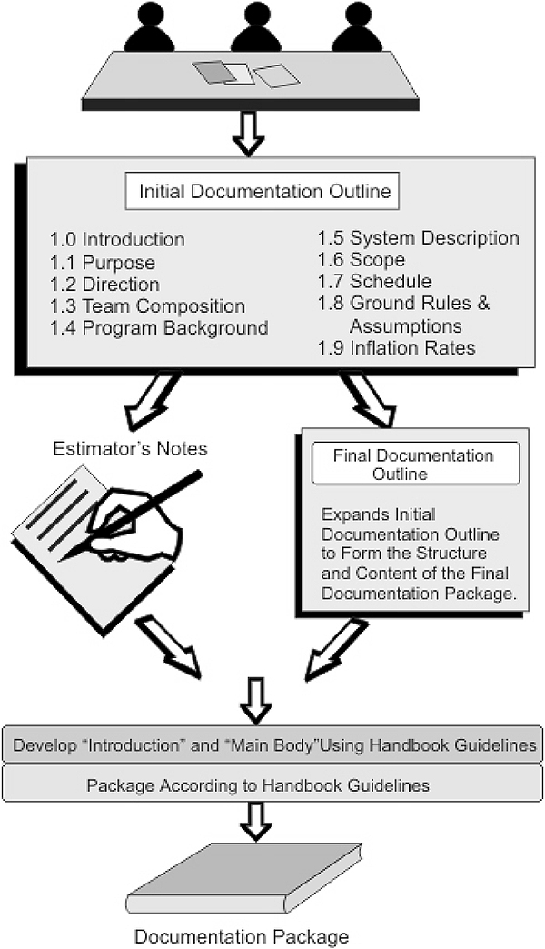
A flow diagram of the documentation process
B11 Cost risk and uncertainty
Poor estimates influence the business and can result in poor business decisions being made. If an estimated project cost is excessively high, then business is likely to be lost as the project will not be priced competitively. Conversely, if the estimated costs are low then profit will be lost because projects are sold at an unattractive margin. Risk and uncertainty exists in cost estimating because a cost estimate is a prediction of the future. There is a chance that the estimated cost may differ from the actual cost. Moreover, the lack of knowledge about the future is only one possible reason for such a difference. Another equally important cause is errors resulting from historical data inconsistencies, cost estimating equations, and factors that typically are used in an estimate. Thus, a cost estimate can include a substantial amount of error. Once this is recognized, the question becomes one of dealing with those errors, which is what the subject of risk and uncertainty is about.
The terms and definitions related to risk and uncertainty analysis are as follows,
- Risk – a situation in which the outcome is subject to an uncontrollable, random event stemming from a known probability distribution.
- Uncertainty – occurs in a situation in which the outcome is subject to an uncontrollable, random event stemming from an unknown probability distribution.
- Engineering Change Orders (ECO) – that amount of money in a program specifically set-aside for uncertainty. ECO generally is referred to as the money set-aside for ‘known-unknowns.’
- Management Reserve (MR) – this term represents a value within the negotiated contract target cost that the contractor has withheld at the management level for uncertainties. Generally, MR is referred to as the money set-aside for ‘unknown-unknowns.’
- Monte Carlo Analysis – a simulation technique, which varies all relevant input parameters to arrive at the potential range of outcomes expressed in terms of probability distributions.
- Sensitivity Analysis – estimating technique in which a relevant non-cost input parameter is varied to determine the probable cost.
- Most Likely Cost – the most likely or most probable estimate of the cost that ultimately will be realized for a program, project, or task.
- Standard Error of the Estimate – represents a measure of the variation around the fitted line of regression, measured in units of the dependent variable.
- Budgeting to Most Likely Cost – the most likely or most probable estimate of the cost that ultimately will be realized for a program, project, or task. Inherent in the estimate should be all funding necessary to ensure that the program can be managed properly in an environment of undefined technical complexity, schedule uncertainty, and the associated cost risk.
- ECO Funding – ECO is the best estimate for contract changes, based on historical precedence (e.g., safety of flight, correction of deficiencies, and value engineering). ECO is a reserve for known-unknown contract changes and does not include reserves for requirements creeping up/down. ECO is an identifiable and traceable element of cost. ECO applies to both development and production and varies by both program and fiscal year.
B11.1 Risk versus uncertainty
The terms risk and uncertainty are often used interchangeably. However, in the more strict definitions of statistics they have distinct meanings. Reviewing these definitions helps clarify the problem confronting the cost estimator.
The traditional view of risk is a situation, in which the outcome is subject to an uncontrollable random event stemming from a known probability distribution, e.g., drawing an ace of spades. Uncertainty is a situation in which the outcome is subject to an uncontrollable, random event stemming from an unknown probability distribution. The general conclusion is that cost estimating is much more in the realm of uncertainty than risk is.
Factors causing uncertainties
The following table provides a listing of John D. Hwang’s findings about the economic, technical, and program factors causing these uncertainties. Generally, these sources of uncertainty are categorized as requirements’ uncertainty and cost estimating uncertainty.
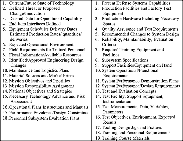
Requirements uncertainty refers to the variation in cost estimates caused by changes in the general configuration or nature of an end item. This would include deviations or changes to specifications, hardware characteristics, program schedule, operational/deployment concepts, and support concepts.
Cost estimating uncertainty refers to variations in cost estimates when the configuration of an end item remains constant. The source of this uncertainty results from errors in historical data, cost estimating relationships, input parameter specification, analogies, extrapolation, or differences among analysts.
Point estimates versus interval estimates
Development of a cost estimate usually involves the application of a variety of techniques to produce estimates of the individual elements of the item. The summation of these individual estimates becomes the singular, best and most likely estimate of the total system and is referred to as a point estimate. The point estimate provides no information about uncertainty other than the value judged more likely to occur compared to any other value. A confidence interval provides a range within which the actual cost should fall, given the confidence level specified.
Uncertainty in decision making
The point estimate provides a best single value, but with no consideration of uncertainty. In contrast, the interval estimate provides significant information about the uncertainty but little about the single value itself. However, when both measures are taken together, they provide valuable information to the decision maker.
An example of the value of this information is in situations involving choice among alternatives, as in the case of source selection. For instance, suppose systems A and B are being evaluated; and because of equal technical merit, the choice will be made on the basis of estimated cost. According to Paul Dieneman, in his report Estimating Cost Uncertainty Using Monte Carlo Techniques, if the choice is made solely on the basis of the most probable cost, the decision may be a poor one (depending upon which of the four situations in Figure B11.1 applies.)

Cost uncertainty in decision making
In situation I, there is no problem in the choice, since all possible costs for A are lower than B. A’s most probable cost is the obvious choice.
Situation II is not quite so clear because there is some chance of A’s costs being higher than B’s. If this chance is low, A’s most probable cost is still the best choice. However, if the overlap is great, then the most probable cost is no longer a valid criterion.
In situation III, both estimates are the same, but the uncertainty ranges are different. At this point, it is the decision maker’s disposition towards risk that decides. If the preference is willingness to risk possible high cost for the chance of obtaining a low cost system, then B is the choice. If the preference is to minimize risk, then A is the appropriate choice.
Finally, situation IV poses a more complicated problem, since the most probable cost of B is lower but with much less certainty than A. If the manager uses only the point estimates in this case, the most probable choice would be the less desirable alternative. In the preceding situations, uncertainty information was a method used to select between alternatives. A quite different use of uncertainty information is when a point estimate must be adjusted for uncertainty.
One particularly effective method of portraying the uncertainty implications of alternative choices is to depict the estimate and its related uncertainty in the form of a cumulative probability distribution, as shown in Figure B11.2 below. The utility of this approach is the easy-to-understand, convenient manner in which the information is presented to the decision maker. In the figure, panel A shows the cost estimate as it might normally be depicted with the most likely value (point estimate at the center); panel B shows the same information in the form of a cumulative curve. It is easy to see, for instance, that the selection of the funding level, F, is at the 75 point, which means that there is only a 25 percent chance of actual cost exceeding this funding level. The manager can see the implications of a particular choice immediately.
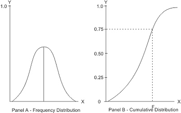
Cumulative probability distribution
Dealing with uncertainty
When actually treating uncertainty in an estimate, several approaches are available, ranging from very subjective judgment calls to rather complex statistical approaches. The order of presentation of these techniques is intentional, because it tends to portray the evolution that has taken place in terms of the tools used to handle uncertainty.
Subjective estimator judgment
This is perhaps one of the oldest methods of accounting for uncertainty and, is the basis for most other approaches. Under this approach the estimator merely reflects upon the assumptions and judgments that were made during the development of the estimate. After evaluating all the ‘ingredients,’ a final adjustment is made to the estimate, usually as a percentage increase. This yields a revised total cost, which explicitly recognizes the existence of uncertainty. The logic supporting this approach is that the estimator is more aware of the uncertainty in the estimate than anyone else, especially if the estimator is a veteran and has experience in systems or items similar to the one being estimated. One method for assisting estimators is to use a questionnaire, which provides a yardstick of their uncertainty beliefs when arriving at their judgment.
Expert judgment/executive jury
It is a technique wherein an independent jury of experts is gathered to review, understand, and discuss the system and its costs. The strengths of this approach are related directly to the diversity, experience, and availability of the group members. The use of such panels or juries requires careful planning, guidance, and control to ensure that the product of the group is objective and reflects the best, unmitigated efforts of each member. Approaches have been designed to contend with the group dynamics of such panels. One classical approach is the Delphi technique, which was originally suggested by RAND. With this technique, a panel of experts is drawn together to evaluate a particular subject and submit their answers anonymously. A composite feedback of all answers is communicated to each panelist, and a second round begins. This process may be repeated a number of times, and ideally, convergence toward a single best solution takes place. By keeping the identities anonymous rather than in a committee session, the panelists can change their minds more easily after each round and provide better assessments, rather than defending their initial evaluation.
The principle drawback of Delphi is that it is cumbersome, and the time elapsed in processing input may present some difficulty to respondents as to their reasons for the ratings. However, it is possible to automate the process with online computer terminals for automatic processing and immediate feedback.
Sensitivity analysis
Another common approach is to measure how sensitive the system cost is to variations in non-cost system parameters. For instance, if system weight is a critical issue, then weight would be varied over its relevant range, and the influence on cost could be observed. Analysis of this type helps to identify major sources of uncertainty.
It also highlights;
- Elements that are cost sensitive,
- Cost obstacles to achieve better program performance, and
- The up gradation possibilities of system performance without increasing program cost substantially.
It does not reveal the extent to which the estimated system cost might differ from the actual cost. It tends to address uncertainty of requirements more than cost uncertainty.
High/low analysis
It requires the estimator to specify the lowest and highest possible values for each system element cost, in addition to its most likely value. These sets of input values are then summed to total system cost estimates. The most likely values establish the central tendency of the system cost, while the sums of the lowest possible values and highest possible values determine the uncertainty range for the cost estimate. It exaggerates the uncertainty of system cost estimates because it is unlikely that all system element costs will be at the lowest (or highest) values at the same time. While the high/low approach is plausible, its shortcoming is that it restricts measurement to three points, without consideration to intermediate values.
Mathematical approaches
Beta and triangular distributions are required to determine the probability distribution for each cost element. Then the individual cost elements are combined and their measures of uncertainty into a total estimate of cost and uncertainty are done by summation of moments and Monte Carlo simulation.
The beta distribution
This distribution is particularly useful in describing cost risk because it is finite, continuous, can easily accommodate a unimodal shape requirement (α > 0, β > 0), and allows virtually any degree of kurtosis and skewness.
Kurtosis characterizes the relative peaks or flats of a distribution as compared to the normal distribution. Skewness characterizes the degree of asymmetry of a distribution around its mean. A few of the many shapes of the Beta are shown in Figure B11.3.

The beta distribution
The Generalized Beta Family of Distributions is defined over an interval (a, a+b) as in Equation below.

In the case of skews,
- When α and β are equal the distribution is symmetric
- When α >β the distribution is negatively skewed
- When α <β the distribution is positively skewed.
Similarly, variance (kurtosis) can be categorized as high, medium, or low, based upon the magnitude of α and β. When these notions of skews and kurtosis are combined, the result is nine combinations as shown in the table below and is translated into the specific beta distributions as shown in the following Figure B11.4.

Specific beta distributions
Triangular distribution
An alternative approach to assigning a distribution shape to a cost element is the triangular distribution and it can take on virtually any combination of skews and kurtosis, but the distribution represented by a triangle rather than the smoother curve of Beta, as shown in figure below. The triangular distribution is specified by the lowest, most likely (usually the point estimate), and the highest value. Any point within the range of the distribution can be chosen to locate the mode and the relationship among the three values specifies the amount of kurtosis. The triangular distribution is much easier to use and produces equally satisfactory results (see Figure B11.5).

The triangular distribution
The summation of moments
This method takes the approach of measuring or describing a distribution through the use of moment statistics. The first moment is the mean (x) and the second, third, and fourth moments (about the mean) take the form of an equation
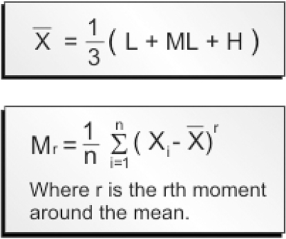
The second moment is the variance. The third and fourth moments are used to calculate two measures that provide additional insight into the shape of a particular distribution.
Those measures are:
- The coefficient of skews, which provides a measure of symmetry
- The coefficient of kurtosis, which measures the peaks or height of a distribution (see B11.6).
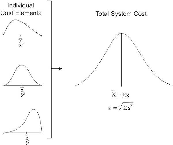
Summation of moments
The critical assumption in this approach is that, the total cost distribution will be normal even though the individual cost element distributions may not be normal. This is shown above.
Monte carlo simulation
An alternative to the summation approach is to use the Monte Carlo Simulation Technique. In this approach, the distribution defined for each cost element (using beta, triangular, or an empirical distribution) is treated as a population from which several random samples are drawn.
For example, a single cost element has been estimated and its uncertainty described as shown in A of Figure below From the probability density function, Y=f(X), a cumulative distribution is plotted, as shown in B of Figure B11.7 below.

Monte Carlo simulation
Qualitative indices of uncertainty
The use of qualitative indices has been proposed as a method of communicating a cost estimate’s goodness, accuracy, or believability. Most of the indices are based upon the quality of the data and the quality of the estimating methodology.
John D. Hwang proposed the rating scheme using a two-digit code with ratings of l to 5 for data and for methodology.
- 1 – highest quality and
- 5 – representing lowest quality. Thus, a rating of 1, 1 would reflect that the estimate was the result of the highest quality level for both. The complete scoring system is shown in Figure B11.8 below.

Qualitative indices of uncertainty
B12 Cost estimation methodology
When choosing a methodology, the cost estimator must always remember that cost estimating is a forecast of future costs based on a logical extrapolation of available historical data. Availability of data is a major factor for selecting the estimation methodology. In addition to availability of data, the type of cost estimating method an estimator chooses will depend on factors such as adequacy of program definition, level of detail required, and time constraints. These factors are all interrelated and shown in Figure B12.1.
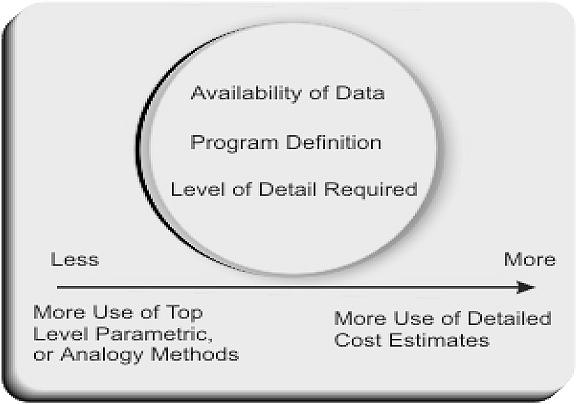
Estimation methodology
B12.1 Parametric estimation
Parametric technology is the ‘best practice’ for estimating. Parametric tools bring speed, accuracy and flexibility to estimating processes, which are often bogged down in bureaucracy and unnecessary detail.
Parametric techniques are a credible cost estimating methodology that can provide accurate and supportable contractor estimates, lower cost proposal processes, and more cost-effective estimating systems.
The parametric method estimates costs based upon various characteristics and attributes of the system being estimated. It depends upon the existence of a casual relationship between system costs and these parameters. Such relationships, known as CERs, typically are estimated from historical data using statistical techniques. If such a relationship can be established, the CER will capture the relationship in mathematical terms relating cost as the dependent variable to one or more independent variables. Examples would be estimating costs as a function of such parameters as equipment weight, vehicle payload or maximum speed, number of units to be produced, or number of lines of software code to be written.
B12.1.1 Overview of parametric estimating
Parametric estimating is the process of estimating cost by using mathematical equations that relate cost to one or more physical or performance characteristics of the item being estimated. A simple example of a parametric estimate is the use of square footage to estimate building costs. Square footage is a physical characteristic of a building that has been shown through statistical analyses of building trends to be one way of estimating building costs. A graphical representation of the complete parametric cost estimating process is shown below. The figure indicates the process from inputs through modeling and into a post processor phase. The post processor allows for the conversion of parametric output into a cost proposal (see Figure B11.2).

Parametric cost estimation
B12.2 Collection and normalization of parametric data
The collecting point for cost and labor hours data is, called the general ledger or a company accounting system. All cost and labor hours data, used in parametric CER’s or cost models, must be consistent with and traceable back to the original collecting point (the source). The data should also be consistent with accounting procedures and cost accounting standards. Technical non cost data comes from engineering drawings, engineering specifications, certification documents, or direct experience (i.e., weighing an item). Schedule, quantity and equivalent units, and similar information comes from Industrial engineering, operations departments, program files or other program intelligence. Any data included in calculating parametric parameters will vary between model developers.
B12.2.1 Significant adjustments to parametric data
There are some of the significant adjustments that may have to be made to historical parametric cost data.
Consistent scope
Adjustments are appropriate for differences in program or product scope between the historical data and the estimate being made.
Anomalies
Historical cost data should be adjusted for anomalies (unusual events), prior to CER analysis, when it is not reasonable to expect these unusual costs to be present in the new projects. The adjustments and judgments used in preparing the historical data for analysis should be fully documented.
Improved technology
Cost changes, due to changes in technology, are a matter of judgment and analysis. All bases for such adjustments should be documented and disclosed.
Inflation
Inflation indices are influenced by internal considerations as well as external inflation rates. Therefore, while generalized inflation indices may be used, it may also be possible to tailor and negotiate indices used on an individual basis to specific labor rate agreements and the actual materials used on the project. It should be based on the cost of materials and labor on a unit basis (piece, pounds, and hour) and should not include other considerations like changes in manpower loading or the amount of materials used per unit of production. The key to inflation adjustments is consistency.
Learning curve
The learning curve analyses labor hours over successive production units of a manufactured item. The curve is defined by the following equation:
Hours/Unit = First Unit Hours × Ub
orFixed Year Cost/Unit = First Unit Cost × Ub
Where: U = Unit number
b = Slope of the curve
In parametric models, the learning curve is often used to analyze the direct cost of successively manufactured units. Direct cost equals the cost of both touch labor and direct materials-in fixed year dollars. Sometimes this may be called an improvement curve. The slope is calculated using hours or constant year dollars.
Production rate
Production rate effects (changes in production rate, i.e., units/months) can be calculated in various ways. For example, by adding another term to the learning or improvement curve equation we would obtain:
Hours/Unit = Ub × Rr
or,Fixed Yr $/Unit = First Unit $ × Ub × Rr
Where:
U = Unit number
b = Learning curve slope
R = Production rate
r = Production rate curve slope
The net effect of adding the production rate effect equation (Rr) is to adjust the First Unit $ for rate. The equation will also yield a different ‘b’ value. The rate effect can vary considerably depending on what was required to effect the change. When preparing a cost estimate, it is preferable to use primary sources of data. The two types of data are:
- Primary data is obtained from the original source. Primary data is considered the best in quality, and ultimately the most useful.
- Secondary data is derived from primary data. It is not obtained directly from the source. Since it was derived (actually changed) from the original data, it may be of lower overall quality and usefulness.
There are nine main sources of data and they are listed in the chart below.
| NINE SOURCES OF DATA | ||
|---|---|---|
| 1. | Basic Accounting Records | Primary |
| 2. | Cost Reports | Either (Primary or Secondary) |
| 3. | Historical Databases | Either |
| 4. | Functional Specialist | Either |
| 5. | Other Organizations | Either |
| 6. | Technical Databases | Either |
| 7. | Other Information Systems | Either |
| 8. | Contracts | Secondary |
| 9. | Cost Proposals | Secondary |
The information needed to use a parametric data model is listed on the chart that follows.
| TYPE OF INFORMATION NEEDED TO USE A PARAMETRIC MODEL |
|---|
| Well-documented Parameters Identifying: |
| Source of data used to derive the parametric model |
| Size of database |
| Time frame of database |
| Range of database |
| How parameters were derived |
| Limitations spelled out |
| How well the parametric model estimates its own database |
| Consistent and well defined WBS dictionary |
| Realistic Estimates of Most Likely Range for Independent Variable Values |
| Top Functional Experts Knowledgeable about The Program You are Estimating |
| To identify most-likely range for cost drivers |
| To confirm applicability of parametric from technical perspective |
B12.2.2 Cost estimating relationships (CERs)
A CER predicts the cost of some part of a program or of the entire program based on specific design or program characteristics. A CER may be used to predict the cost of an entire project.
Definition: Cost Estimating Relationships (CERs) are mathematical expressions relating cost as the dependent variable to one or more independent cost driving variables.
Types of CERs
CERs can be divided into several classes depending on:
- The kind of costs to be estimated
- The cost drivers chosen to predict costs
- The complexity of the estimating relationship
- The aggregation level of the CER
The kind of costs to be estimated can be grouped into the three phases of a program’s life cycle:
- Research, engineering and development (RE&D)
- Production
- Operating and support (O&S).
CERs classified by type of cost driver
The type of cost driver also classifies CERs. Cost estimators have discovered a variety of quantitative cost drivers to apply to CERs. The most common variable for hardware remains weight.
CERs classified by aggregation level
CERs can be classified in terms of the aggregation level of the estimate. For instance, CERs can be developed for the whole system, major subsystems, other major non-hardware elements (training, data, etc.) and components. The aggregation level of the cost drivers, as shown in Figure B12.3, should match the aggregation level of the costs to be estimated.

Matching aggregation levels of CERs
Uses of CERs
CERs are used to estimate costs at many points in the acquisition cycle when little is known about the cost to be estimated. CERs are of greatest use in the early stages of a system’s development and can play a valuable role in estimating the cost of a design approach.
CERs can serve as checks for reasonableness on bids proposed by contractors. Even after the start of the development and production phases, CERs can be used to estimate the costs of non-hardware elements. For example, they can be used to make estimates of O&S costs. This may be especially important when trying to determine downstream costs of alternative design, performance, logistic, or support choices that must be made early in the development process.
Developing CERs
A CER is a mathematical equation that relates one variable such as cost (a dependent variable) to one or more other cost drivers (independent variables). The objective of constructing the equation is to use the independent variables about which information is available or can be obtained to predict the value of the dependent variable that is unknown. When developing a CER, the analyst must first hypothesize a logical estimating relationship. After developing a hypothetical relationship, the analyst needs to assemble a database.
Hypothesis testing of a logical CER
The analyst must structure the forecasting model and formulate the hypothesis to be tested. The work may take several forms depending upon forecasting needs. It involves discussions with engineers to identify potential cost driving variables, scrutiny of the technical and cost proposals, and identification of cost relationships. Only with an understanding of hardware requirements can an analyst attempt to hypothesize a forecasting model necessary to develop a CER.
The CER model
Once the database is developed and a hypothesis determined, the analyst is ready to mathematically model the CER – both linear and curvilinear, considering one simple model – the LSBF model.
When to use a CER
When a CER has been built from an assembled database based on a hypothesized logical statistical relationship, one is ready to apply the CER. It may be used to forecast future costs or it may be used as cross checks of an estimate done with another estimating technique. CERs are a fundamental estimating tool used by cost analysts.
Strengths and weaknesses of CER’S
Some of the more common ones are presented below:
Strengths
- One of the principle strengths of CERs is that they are quick and easy to use. Given a CER equation and the required input data, one can generally turn out an estimate quickly.
- A CER can be used with limited system information. Consequently, CERs are especially useful in the RDT&E phase of a program.
- A CER is an excellent (statistically sound) predictor if derived from a sound database, and can be relied upon to produce quality estimates.
Weaknesses
- CERs are sometimes too simplistic to forecast costs. Generally, if one has detailed information, the detail may be reliably used for estimates. If available, another estimating approach may be selected rather than a CER.
- Problems with the database may mean that a particular CER should not be used. A cost model should not be used without reviewing its source documentation.
Regression analysis
The purpose of regression analysis is to improve the ability to predict the next ‘real world’ occurrence of our dependent variable. Regression analysis may be defined as the mathematical nature of the association between two variables. The association is determined in the form of a mathematical equation. Such an equation provides the ability to predict one variable on the basis of the knowledge of the other variable. The variable whose value is to be predicted is called the dependent variable. The variable about which knowledge is available or can be obtained is called the independent variable. The dependent variable is dependent upon the value of independent variables. The relationships between variables may be linear or curvilinear. By linear, the functional relationship can be described graphically (on a common X-Y coordinate system) by a straight line and mathematically by the common form:
y = a + bx
where y = (represents) the calculated value of y – the dependent variable
x = the independent variable
b = the slope of the line, the change in y divided by the corresponding change in x.
a and b are constants for any value of x and y.
For the bi-variate regression equation – the linear relationship of two variables can be described by an equation, which consists of two distinctive parts, the functional part and the random part. The equation for a bi-variate regression population is:
Y = A + BX + E
where;
A + BX is the functional part (a straight line) and E is the random part.
A and B are parameters of the population that exactly describe the intercept and slope of the relationship.
E represents the ‘error’ part of the equation i.e., the errors of assigning values, the errors of measurement, and errors of observation due to human limitations, and the limitations associated with real world events.The above equation is adjusted to the form:
y = a + bx + e,
where;
a + bx represents the functional part of the equation and e represents the random part.
Curve fitting
There are two standard methods of curve fitting. One method has the analyst plot the data and fit a smooth curve to the data. This is known as the graphical method. The other method uses formulas or a ‘best-fit’ approach where an appropriate theoretical curve is assumed and mathematical procedures are used to provide the one ‘best-fit’ curve; this is known as the Least squares best fit (LSBF) method.
We are going to work the simplest model to handle, the straight line, which is expressed as:
Y = a + bx
Graphical method
To apply the graphical method, the data must first be plotted on a graph paper. No attempt should be made to make the smooth curve actually pass through the data points which have been plotted; rather, the curve should pass between the data points leaving approximately an equal number of points on either side of the line. For linear data, a clear ruler or other straightedge may be used to fit the curve. The objective in fitting the curve, i.e. to ‘best-fit’ the curve to the data points plotted; that is, each data point plotted is equally important and the curve you fit must consider each and every data point.
LSBF method
The LSBF method specifies the one line, which best fits the data set we are working with. The method does this by minimizing the sum of the squared deviations of the observed values of Y and calculated values of Y i.e., (Y1 − YC1)2 + (Y2 − YC2)2 + (Y3 − YC3)2 + … + (Yn − YCn)2 (see Figure B12.4).
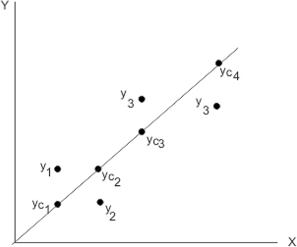
LSBF line
Therefore, the LSBF line is one that can be defined as:
ΣE2 is a minimum because Σ (Y − YC)2 = ΣE2For a straight line,
Y = a + bx
and, with N points,The sum of the squares of the distances is a minimum if,
ΣY = AN + BΣX and
ΣXY = AΣX + BΣX2
These two equations are called the normal equations of the LSBF line. LSBF regression properties are:
- The technique considers all points.
- The sum of the deviations between the line and observed points is zero.
- Now, the LSBF regression line intercepts the Y-axis at a distance ‘a’ and with a slope of ‘b’. A spreadsheet is used for the calculation.
Table Needed to Get Sums, Squares and Cross Products
| X | Y | X×Y | X2 | Y2 |
| X1 | Y1 | X1 × Y1 | X12 | Y12 |
| X2 | Y2 | X2 × Y2 | X22 | Y22 |
| X3 | Y3 | X3 × Y3 | X32 | Y32 |
| – | – | – | – | – |
| – | – | – | – | – |
| ΣXn | ΣYn | Σ(Xn × Yn) | ΣXn2 | ΣYn2 |
| X | Y | X Y | X2 | Y2 |
| 4 | 10 | 40 | 16 | 100 |
| 11 | 24 | 264 | 121 | 576 |
| 3 | 8 | 24 | 9 | 64 |
| 9 | 12 | 108 | 81 | 144 |
| 7 | 9 | 63 | 49 | 81 |
| 2 | 3 | 6 | 4 | 9 |
| 36 | 66 | 505 | 280 | 974 |
where

Therefore, the regression equation (calculated y) is

Multiple regressions
In simple regression analysis, a single independent variable (X) is used to estimate the dependent variable (Y), and the relationship is assumed to be linear (a straight line). This is the most common form of regression analysis used in contract pricing. However, there are more complex versions of regression equations that can be used to consider the effects of more than one independent variable on Y. That is, multiple regression analysis assumes that the change in Y can be better explained by using more than one independent variable. For example, the number of miles driven may largely explain automobile gasoline consumption. However, it might be better explained if we also considered factors such as the weight of the automobile. In this case, the value of Y would be explained by two independent variables.
Yc = A + B1X1 + B2X2
where:
Yc = the calculated or estimated value for the dependent variable
A = the Y intercept, the value of Y when X = 0
X1 = the first independent (explanatory) variable
B1 = the slope of the line related to the change in X1, the value by which change when X1 changes by one
X2 = the second independent variable
B2 = the slope of the line related to the change in X2, the value by which change when X2 changes by one.
Curvilinear regression
In some cases, the relationship between the independent variable(s) may not be linear. Instead, a graph of the relationship on ordinary graph paper would depict a curve.
‘Goodness’ of fit, R and R2
After the development of the LSBF regression equations, now we need to determine how good a forecast we will get by using our equation. In order to answer this question, we must consider a check for the ‘goodness’ of fit, the coefficient of correlation (R) and the related coefficient of determination (R2).
Correlation analysis
One indicator of the ‘goodness’ of fit of a LSBF regression equation is correlation analysis. Correlation analysis considers how closely the observed points fall to the LSBF regression equation and more closely the observed values are to the regression equation, the better the fit; hence, the more confidence in the forecasting capability. Correlation analysis refers only to the ‘goodness’ of fit or how closely the observed values are to the regression equation but nothing about cause and effect.
Coefficient of determination
The coefficient of determination (R2) represents the proportion of variation in the dependent variable that has been explained or accounted for by the regression line. The value of the coefficient of determination may vary from zero to one. A coefficient of determination of zero indicates that none of the variation in Y is explained by the regression equation; whereas a coefficient of determination of one indicates that 100 percent of the variation of Y has been explained by the regression equation. Graphically, when R2 is zero, the observed values appear as in Figure B12.7 (bottom) and when the R2 is one, the observed values all fall right on the regression line as in Figure B12.8 (top).

Coefficient of determination
In order to calculate R2 we need to use the equation:

R2 tells us the proportion of total variation that is explained by the regression line. Thus R2 is a relative measure of the ‘goodness’ of fit of the observed data points to the regression line. If the regression line perfectly fits all the observed data points, then all residuals will be zero, which means that R2 = 1.00. The lowest value of R2 is 0, which means that none of the variation in Y is explained by the observed values of X.
Coefficient of correlation
The coefficient of correlation (R) measures both the strength and direction of the relationship between X and Y. R takes the same sign as the slope; if b is positive, use the positive root of R2 and vice versa. For example, if R2 = 0.81; then R = ±0.9 and we determine whether R takes the positive root (+) or the negative root (−) by noting the sign of b. If b is negative, then we use the negative root of R2 to determine R. So to calculate R it is required to know the sign of the slope of the line. R only indicates the direct / an inverse relationship and the strength of the association.
Learning curve effect
Wright first observed the learning curve in the 1930s in the American aircraft industry, and Crawford confirmed his pioneering work in the 1940s. The learning effect is not concerned with reduction in unit cost as production increases and /or production facilities are scaled up to manufacture larger batches of products.
Learning effect
The learning effect is concerned with cumulative production over time-not the manufacture of a single product/batch at a particular moment in time-and recognizes that it takes less time to assemble a product, the more that product is made by the same worker, or group of workers. That is the learning effect.
Cost reduction tool
It is important to appreciate that the learning curve is not a cost-reduction technique since the learning curve model can predict the rate of future time reduction accurately. Cost reduction only occurs if management action is taken, for example, to increase the rate of time reduction by providing additional training, provision of better tools etc. The learning effect occurs because people are inventive, learn from earlier mistakes, and are generally keen to take less time to complete tasks, for a variety of reasons. It should also be noted that the learning process might be done consciously and/or intuitively. The learning curve consequently reflects human behavior.
Learning curve sectors
While the learning curve can be applied to many sectors, its impact is most pronounced in sectors, which have repetitive, complex operations where people principally determine the pace of work, not machines. Examples of sectors where the learning effect is pronounced include:
- Aerospace
- Electronics
- Shipbuilding
- Construction
- Defense
The learning curve is also being utilized by rail operators; for example, seek to extend cost-effectively the lives of their assets. Another sector, which makes considerable use of this technique, is the space industry. NASA uses the learning curve to estimate costs for the production of space shuttles, time to complete tasks in space etc.
Learning curve model
Wright observed that the cumulative average time per unit decreases by a fixed percentage each time cumulative production doubles over time. The following table illustrates this effect:

The above table indicates that the cumulative average time per unit falls by 10% each time cumulative production doubles, i.e. it is depicting a 90% learning curve. The above relationship between cumulative output and time can be represented by the following formula:
Basic form of the ‘learning curve’ equation is,
y = a.xb or, Log y = Log a + b Log x
where,
y = Cost of Unit #x (or average for x units)
a = Cost of first unit
b = Learning curve coefficient
The equation Log y = Log a + b Log x is of precisely the same form as the linear equation y = a + bx. This means that the equation Log y = Log a + b Log x can be graphed as a straight line on log-log graph paper and all the regression formulae apply to this equation just as they do to equation y = a + bx. In order to derive a learning curve from cost data (units or lots) the regression equations need to be used whether or not the calculations are performed manually or using a statistical package and the learning curve equation is a special case of the LSBF technique.
Since in learning curve methodologies cost is assumed to decrease by a fixed amount each time quantity doubles, then this constant is called the learning curve ‘slope’ or percentage (i.e., 90%). For example,
For unit #1
Y1 = A (1) b = A (First Unit Cost) and
For unit #2
Y2 = A (2) b = Second Unit CostSo,
Y2/ Y1 = A. (2) b / A = 2b = a Constant, or ‘Slope’
Slope = 2b, and, Log Slope = bLog2Therefore, b = Log Slope/ Log2
For a 90% ‘Slope,’
b = Log.9/ Log 2 = −0.152If we assume that A = 1.0, then the relative cost between any units can be computed.
Y3 = (3)−0.152 = 0.8462
Y6 = (6)−0.152 = 0.7616Note that:
Y6 /Y3 = .7616 /.8462 = 0.9
Statistical package i.e., Stat View can perform all the calculations shown and greatly simplified using these tools.
Decision-making
While a great deal has been written about the use of the learning curve for control purposes, this technique can also be used to determine costs for potential contracts in sectors, which exhibit the learning effect. For example, Above & Beyond Ltd, which produces high-technology guidance systems, is preparing a tender for the Aurora project, the new generation of space shuttles. The guidance systems for the Aurora project will be very similar to those recently supplied by the company for the Dark Star project, experimental Stealth aircraft capable of flying outside the earth’s atmosphere. The company has been asked to submit a tender to install ten guidance systems for this project. While a tender would take account of all costs that would apply to a particular project, one of the key costs for a high-technology project is labor time, as highly skilled personnel (who are highly paid) are required to assemble and test such systems. The following analysis will focus on the labor time required for this project.
Aurora project
Above & Beyond Ltd’s engineers believe it is possible to estimate the time required to install the guidance systems for the new generation of space shuttles from the learning derived from the Dark Star project. The same system will be installed in the space shuttles. The following data was consequently obtained in respect of the Stealth project:
- Time to install first system: 12,000 hours
- Total installed: to date 9 systems
- Total cumulative time: 69,595 hours.
The first figure to be calculated is b, the index of learning, and this can be derived from the learning curve equation, Yx = ax b, since all the other figures are known.

It is now possible to estimate the time required to install the guidance systems for this project.

Please note that the learning curve would produce an estimate of 75,715 hours to install the guidance systems using a learning rate of 87% if no account was taken of the learning derived from Dark Star. This difference of 18,783 hours is extremely significant since the costs of hiring specialist engineers, and supporting these engineers, could be £100+ per hour, i.e. £1.8m+.
Limitations, errors and caveats of LSBF techniques
- Extrapolation
A LSBF equation is truly valid only over the same range as the one from which the sample data was initially taken. - Cause and Effect
Regression and correlation analysis can in no way determine cause and effect.
Illustration of CER use
Assume an item of equipment in 1980 cost $28,000 when an appropriate Consumer Price Index (CPI) was 140. If the current index is now 190 and an offer to sell the equipment for $40,000 has been suggested, how much of the price increase is due to inflation? How much of the price increase is due to other factors?
Solution
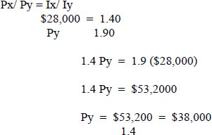
$38,000 now is roughly the equivalent of $28,000 in 1980. Hence the price difference due to inflation is $38,000 − $28,000 = $10,000. The difference due to other causes is $2,000 ($40,000 − $38,000).
The above example would illustrate the use of CPI numbers for a material cost analysis. The steps were:
- If we know what the price of an item was in the past, and we know the index numbers for both that time period and today, we can then predict what the price of that item should be now based on inflation alone.
- If we have the same information as above, and we have a proposed price, we can compare that price to what it should be based on inflation alone. If the proposed price is higher or lower than we expect with inflation, then we must investigate further to determine why a price or cost is higher or lower.
Illustration:
A house to be purchased. Historical data for other houses purchased, may be examined during an analysis of proposed prices for a newly designed house. Table below shows data collected on five house plans so that we can determine a fair and reasonable price for a house of 2100 square feet and 2.5 baths.
| House Model | Unit Cost | Baths | Sq. Feet Living Area |
Sq. Feet Exterior Wall Surface |
| Burger | 166,500 | 2.5 | 2,800 | 2,170 |
| Metro | 165,000 | 2.0 | 2,700 | 2,250 |
| Suburban | 168,000 | 3.0 | 2,860 | 2,190 |
| Executive | 160,000 | 2.0 | 2,440 | 1,990 |
| Ambassador | 157,000 | 2.0 | 1,600 | 1,400 |
| New House | Unknown | 2.5 | 2,600 | 2,100 |
Solution:
Using this data, we can demonstrate a procedure for developing a CER.
Step 1: Designation and definition of the dependent variable. In this case we will attempt to directly estimate the cost of a new house.
Step 2: Selection of item characteristics to be tested for estimating the dependent variable. A variety of home characteristics could be used to estimate cost. These include such characteristics as: square feet of living area, exterior wall surface area, number of baths, and others.
Step 3: Collection of data concerning the relationship between the dependent and independent variable.
Step 4: Building the relationship between the independent and dependent variables.
Step 5: Determining the relationship that best predicts the dependent variable.
Figure B12.8 graphically depicts the relationship between the number of baths in the house and the price of the house. The relationship may not be a good estimating tool, since three houses with a nearly $8,000 price difference (12 percent of the most expensive house) have the same number of baths.

Relationship between number of baths and prices of a house
Figure B12.9 graphically relates square feet of living area to price. In this graph, there appears to be a strong linear relationship between house price and living area.

Square feet of living area to price
Figure B12.10 graphically depicts the relationship between price and exterior wall surface area. Again, there appears to be a linear relationship between house price and this independent variable.
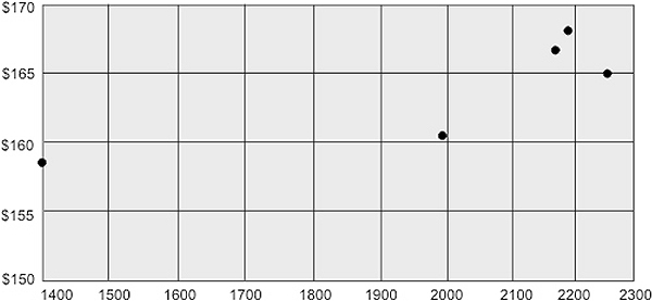
Relationship between price and exterior wall surface area
Based on this graphic analysis, it appears that square feet of living area and exterior wall surface have the most potential for development of a cost estimating relationship. We may now develop a ‘line-of-best-fit’ graphic relationship by drawing a line through the average of the x values and the average of the y values and minimizing the vertical distance between the data points and the line (Figure B12.11 and B12.12).

Linear trend of cost to living area (Sq. Ft.)
Viewing both these relationships, we might question whether the Ambassador model data should be included in developing our CER. However, we should not eliminate data just to get a better-looking relationship. Here, we find that the Ambassador’s size is substantially different from the other houses for which we have data and price estimation. This substantial difference in size might logically affect the relative construction cost. The trend relationship using the data for the four other houses would be substantially different than relationships using the Ambassador data. Based on this information, we may decide not to consider the Ambassador data in CER development.

Linear trend of cost to exterior wall surface (Sq. Ft.)
If we eliminate the Ambassador data, we will find that the fit of a straight-line relationship of price to the exterior wall surface is improved.

Relationship of price to square feet of living area
If we have to choose one relationship, we would probably select the one shown in the table (square feet of living area) over the relationship involving exterior wall surface because there is so little variance shown about the trend line. If the analysis of these characteristics does not reveal a useful predictive relationship, we may consider combining two or more of the characteristics already discussed, or explore new characteristics. However, since the relationship between living area and price is so close, we may reasonably use it for our CER.
In documenting our findings, we can relate the process involved in selecting the living area for price estimation. We can use the graph developed as an estimating tool. The cost of the house could be calculated by using the same regression analysis formula discussed herein:
| For square feet of living area: | Y = $117,750 + $17.50 (2600) |
| Y = $117,750 + $45,500 | |
| Y = $163,250 estimated price |
Common CERS
A list of some common CERs used to predict prices or costs of certain items are given below. In addition to CERs used for estimating total cost and prices, others may be used to estimate and evaluate individual elements of cost. CERs are frequently used to estimate labor hours. Tooling costs may be related to production labor hours, or some other facet of production. Other direct costs may be directly related to the labor effort involved in a program.

A flow chart of the CER development process is shown in Figure B12.14.

CER development process
B12.3 Analogy cost estimation
Analogy cost estimates (also called comparative cost estimates) is characterized by use of a single historical data point serving as the basis for a cost estimate. A program cost estimate identified as an analogy cost estimate consists of more than one, and often many. As estimates are based on extrapolation of a single data point, the comparison or extrapolation process is critical. Use of analogy estimating methods is advisable when the new system is primarily a combination of existing subsystems, equipment, or components for which recent and complete historical cost data are available. Analogy methods are most useful in situations where rapidly advancing technology and acquisition strategies cause a parametric cost model database to become outdated quickly. A properly completed and documented analogy estimate provides a good understanding of how the program description affects the estimate produced. Since analogy cost estimates can be prepared quickly these methods are often used to check other methods.
When analogy cost estimating methods is employed, the new system is broken down into components, which are compared to similar existing components. The basis for comparison can be in terms of capabilities, size, weight, reliability, material composition, or design complexity. Analogy cost estimating usually requires the services of technical specialists.
B12.3.1 Key analogy estimate activities
Key activities involved in making an analogy estimate are shown in the Fig-69. Each block represents an activity. Arrows indicate the usual sequence of activities and dashed lines indicate interactive activities. Some activities must be repeated for each of the several system components. Factors are likely to be developed once and used for all or most components. Many analogy estimates are less complex than indicated in the figure, especially if only one cost element is included. When only a single item is involved, the critical activities (L, M, and N) need to be performed only once. There also is reduced work associated with activities A through F and J.
Many activities shown in Figure B12.15 are not unique to analogy estimates.
Each block in the figure has a letter in the upper right corner to key it to its associated paragraph in the following text.
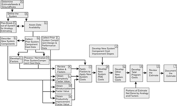
Analogy estimate activities
Activity A
Determine estimate needs and ground rules
Cost estimates differ widely from detailed life cycle cost estimates, which cover activities occurring over periods up to 20 years, to simple estimates for a one time purchase of a single piece of equipment hardware of an existing design. Estimates differ by level of detail or accuracy required. Some estimates need to be detailed so that costs can be tracked and managed at a lower level. Ground rules and assumptions e.g., inflation rates to be used, buy quantities, schedules, interactions with other programs, test requirements, etc. must be defined. Estimate objectives, assumptions, and ground rules should be documented at the outset and agreed upon by all, especially program management.
Activity B
Define the system
Defining the system includes determining:
- Design or physical parameters such as weight, size, material type, and design approach
- Required performance characteristics such as speed, range, computation speed, reliability and maintainability
- Interface requirements with other systems, equipment, and organizations
- Unusual training, operations, and support requirements
- Unusual testing or certification requirements
- Level of technology advance, if any, required
- Known similar systems.
Activity C
Plan breakout of system for analogy estimating
The overall objective of this activity is to break out the overall system into components in the following way:
- Good comparable components from past programs can be identified.
- Relatively complete cost and descriptive data on the components from past programs are available.
- Technical experts who have or can quickly obtain a good understanding of the differences between the old and new system components are available.
Activity D
Assess data availability
Three types of data are required:
- Quantity, design, and performance characteristics of the new system components
- Quantity, design, and performance characteristics for components of one or more prior systems
- Cost data for the prior system components.
Activity E
Describe the new system components
Once plans for the breakout are sound, the next step is to describe each of the new system components in terms of most comparable, to prior system components and which are more likely to reflect cost differences. It is important that similar information can be found for the prior system components.
Activity F
Collect prior system component design and performance data
It is preferable to gather measurable recent data on several characteristics for each component and must be in terms comparable with the information known about the new system.
Activity G
Collect prior system component cost data
The prior system component cost data must be for the same items for which the design and performance data was collected. Cost values should explain the following requirements:
- What is included in the cost (e.g., software, etc.)?
- What year dollars the cost values are in and when the work included in the costs was completed?
- What general and administrative (G&A) costs and profit were included in the values?
- Where in the sequence of units bought were the items to which the cost values apply?
- A breakout of recurring and nonrecurring production costs
- Cost improvement curve slope values experienced during production of the prior system components.
Activity H
Process/Normalize prior system component cost data
The objective of processing the prior system component cost data is to obtain the following:
- All cost values in a common constant year
- A breakout of all nonrecurring costs from recurring costs
- A breakout of full-scale development (FSD), and production costs, if a developmental program
- Recurring production cost improvement slopes and curve types
- Knowledge of prototype to first production unit cost improvement curve step functions, if any, associated with prior system component production
- Knowledge of anything unusual about prior system costs or uncertainties concerning the cost values obtained
- Nonrecurring to recurring cost ratios.
Activity I
Develop factors based on prior system costs
Sometimes, extrapolating cost elements from past systems to future systems is more logical than using design and performance differences as a basis. It is advisable to check the factors developed with similar ones used for other estimates and reconcile any major differences.
Activity J
Develop the new system component cost improvement slope values
This is applicable only if there is recurring production or production of multiple prototypes involved.
Activity K
Review ratios and factors
When preparing analogy estimates, cost estimators generally need to rely on judgments made by engineers and other technical specialists because of their knowledge of both the new and prior programs. They review the ratios and factors developed in Activity H and Activity I.
Activity L
Obtain complexity factor values
This activity is the foundation of analogy estimating methodology and result in an understandable and traceable reason for each complexity factor developed.
Activity M
Obtain miniaturization factor values
The smaller the subsystem is for a given level of performance, the more costly it is to produce. The question of ‘how much more’ should be presented in terms of the ratio of the expected cost of the new system to the expected cost of designing a new system with the same level of performance but with no space and weight constraints.
Activity N
Obtain productivity improvement factor values
Productivity improvements should drive costs down or at least somewhat offset inflation cost increases. Technical specialists should be asked if there has been significant productivity improvement between production of the prior and new systems. It is very desirable to obtain separate factor judgments for complexity, miniaturization, and productivity changes.
Activity O
Apply factors to obtain new system costs
In applying the factors, the following equation is used. Where two or more factors are combined, the equation will change accordingly.
CN = CP × FC × FM × FP
where
CN = the equivalent cost for the new system
CP = any T1, FSD, or production nonrecurring cost for the prior system or system component
FC = Complexity factor ratio
FM = Miniaturization factor ratio
FP = Productivity component ratio
Activity P
Develop new system PME cost estimates
Recurring and nonrecurring costs are added to develop total prime mission equipment (PME) costs for each WBS component addressed. Costs for the various components or groups of components involved are summed to get the total new system PME cost for FSD and the specified production quantity of interest.
Activity Q
Develop other new system costs with factors
A common approach is to use the differences in characteristics to extrapolate from the PME costs of prior systems to the PME costs of the new system. When this is done, other elements of cost such as Systems engineering/Program management, spares, support equipment, training, and data must be added to complete the estimate for the new system.
Activity R
Develop total program costs
Completion of activities P and Q should provide cost data that can be summed to get the total cost for a contractor to provide the new system. If the program has several contractors, the total program cost must combine the costs associated with all contractors.
Activity S
Review the estimate
Analogy cost estimates should be reviewed before preparing final documentation and is best performed by other cost estimators or supervisors experienced in analogy cost estimating.
Activity T
Document the estimate
Analogy cost estimate documentation has much in common with documentation required for any cost estimate.
Engineering estimating
This method generally involves a more detailed examination of the new system and program. Engineering estimates prepared by contractors usually do not include other government costs and engineering change costs. Most significant estimating efforts are a combination of several methods and the best combination of methods is the one which makes the best possible use of the most recent and applicable historical data and system description information and which follows sound logic to extrapolate from historical cost data to estimated costs for future activities. The smaller the extrapolation gap in terms of technology, time, and activity scope the better.
B12.4 Estimation formulas
Cost estimates are often based on a single variable representing the capacity or some physical measure of the design such as floor area in buildings, length of highways, volume of storage bins and production volumes of processing plants. Costs do not always vary linearly with respect to different facility sizes. If the average cost per unit of capacity is declining, then scale economies exist. Conversely, scale diseconomies exist if average costs increase with greater size. Let x be a variable representing the facility capacity, and y be the resulting construction cost. Then, a linear cost relationship can be expressed in the form:

Where a and b are positive constants to be determined on the basis of historical data. A fixed cost of y = a, at x = 0 is implied as shown in Figure B12.18. In general, this relationship is applicable only in a certain range of the variable x, such as between x = c and x = d. If the values of y corresponding to x = c and x = d are known, then the cost of a facility corresponding to any x within the specified range may be obtained by linear interpolation.

Linear cost relationship with economies of scale
A nonlinear cost relationship between the facility capacity x and construction cost y can often be represented as:

Taking the logarithm of both sides in this equation, a linear relationship can be obtained as follows:

A nonlinear cost relationship often used in estimating the cost of a new industrial processing plant from the known cost of an existing facility of a different size is known as the exponential rule. Let yn be the known cost of an existing facility with capacity Qn, and y be the estimated cost of the new facility, which has a capacity Q.

where m usually varies from 0.5 to 0.9, depending on a specific type of facility. A value of m = 0.6 is often used for chemical processing plants.
The exponential rule can be reduced to a linear relationship if the logarithm of Equation is used:

The exponential rule can be applied to estimate the total cost of a complete facility or the cost of some particular component of a facility.

Cost indexes
An index is a dimension-less number that indicates how a cost or a price has changed with time (typically escalated) with respect to a base year. It shows how prices / costs vary with time-a measurement of inflation or deflation. Changes usually occur as a result of:
- Technological advances
- Availability (scarcity) of labor and materials
- Changes in consumer buying patterns
It establishes a reference from some base time period (i.e., a base year). When compared to a current-year index measures the amount (%) change from the base period.
Examples:
Engineering News-Record Construction Index
Producer Prices and Price Indexes
Consumer Price Index Detailed Report
Yn = Yk (In/Ik)
where:
Yn = estimated cost or price of item in year n
Yk = cost or price of item in year k for k < n
In = index value in year n
Ik = index value in year k
Developing indexes
For a single item, the index value is simply the ratio of the cost of the item in the current year to the cost of the same item in the reference year, multiplied by the reference year factor.
Averaging the ratios of selected item costs in a particular year to the cost of the same items in a reference year can create a composite index. Weights can be assigned to the items according to their contribution to total cost.
Unit technique
Utilizes a ‘per unit’ factor that can be estimated effectively.
- Construction cost per square foot
- Operating cost per mile
- Maintenance cost per hour
Suppose that a project is decomposed into n elements for cost estimation. Let Qi be the quantity of the ith element and ui is the corresponding unit cost. Then, the total cost of the project is given by:

where n is the number of units.
Factor technique
An extension of the unit method where the sum of products of component quantities and corresponding unit costs plus component costs is estimated directly.

where:
| C | = | cost being estimated |
| Cd | = | cost of the selected component d that is estimated directly |
| fm | = | cost per unit of component m |
| Um | = | number of units of component m |
B12.5 Power sizing
This estimating model assumes that cost varies as some power of the change in size or capacity. Also referred to as exponential model, which are used for costing plants and equipment. Recognizes that cost varies as some power of the change in capacity or size.
(CA / CB) = (SA / SB)X
where:
| CA | = | cost for item A |
| CB | = | cost for item B |
| SA | = | size of item A |
| SB | = | size of item B |
| X | = | cost-capacity factor |
Illustration
The total construction cost of a refinery with a production capacity of 200,000 bbl/day in Indiana, completed in 2001 was $100 million. It is proposed that a similar refinery with a production capacity of 300,000 bbl/day be built in California, for completion in 2003. For the additional information given below, make an order of magnitude estimate of the cost of the proposed plant.
- In the total construction cost for the Indiana plant, there was an item of $5 million for site preparation, which is not typical for other plants.
- The variation of sizes of the refineries can be approximated by the exponential rule, with m = 0.6.
- The inflation rate is expected to be 8% per year from 1999 to 2003.
- The location index was 0.92 for Indiana and 1.14 for California in 1999. These indices are deemed to be appropriate for adjusting the costs between these two cities.
- New air pollution equipment for the LA plant costs $7 million in 2003 dollars (not required in the Indiana plant).
- The contingency cost due to inclement weather delay will be reduced by the amount of 1% of total construction cost because of the favorable climate in LA (compared to Indiana).
Solution
On the basis of the above conditions, the estimate for the new project may be obtained as follows:
Typical cost excluding special item at Indiana is
$100 million − $5 million = $95 millionAdjustment for capacity based on the exponential law yields
($95)(300,000/200,000)0.6 = (95)(1.5)0.6 = $121.2 millionAdjustment for inflation leads to the cost in 2003 dollars as
($121.2)(1.08)4 = $164.6 millionAdjustment for location index gives
($164.6)(1.14/0.92) = $204.6 millionAdjustment for new pollution equipment at the California plant gives
$204.6 + $7 = $211.6 millionReduction in contingency cost yields
($211.6)(1−0.01) = $209.5 million
Since there is no adjustment for the cost of construction financing, the order of magnitude estimate for the new project is $209.5 million.
B12.6 Case studies
1. Based on driving 15,000 miles per year, the average annual cost of owning and operating a 4-cylinder automobile in 1998 is estimated to be $0.42 per mile. The cost breakdown is shown below.
- Depreciation: $0.210
- Gasoline and oil: $0.059
- Finance charges (based on 20% down and 48 months financing at A.P.R.): $0.065
- Insurance costs (including collision): $0.060
- Taxes, license and registration fees: $0.015
- Tire costs: $0.011
(a) If a person who owns this ‘average’ automobile plans to drive 15,000 miles during 1998, how much would it cost to own and operate the automobile?
(b) If the person actually drives 30,000 miles in 1998, give some reasons why his/her actual cost may not be twice the answer obtained in part (a).
(c) Attempt to develop an estimate of the cost per mile of owning and operating this automobile in the year 2002.
2. You must build a new and larger factory. You know those 30 years ago, it cost $10 million to build a 10,000 sq ft facility. Today, you wish to build a 20,000 sq ft facility. Assume that the cost index was 200, 30 years ago and is 1,200 today. Let X = 0.6. What is the cost to build the new and larger factor?
B12.7 Construction projects and taking off materials from drawings
Types
- Building construction projects – Residential and non-residential
Labor intensive and architectural design
- Heavy and highway projects – Roads and bridges, dams and canals and power plants
Equipment intensive and engineering design
- Industrial construction – Factories and refineries
Types of contractors
- Residential Contractor
- General Building Contractor
- Specialty Contractor (Subcontractors)
- Heavy and Highway Contractor
B12.7.1 Project estimation
Determination of quantities of materials, equipment, and labor for a given project and apply proper unit costs to these items.
Why estimation?
To estimate,
- The probable real cost to build a project (direct costs, indirect costs, contingency, profit)
- The probable real time to build a project (activity duration and project duration)
Construction phases and type of estimates

Feasibility estimates
- May be based on total cost of project, including land cost, professional fess, finance cost, construction cost, and operating costs
- Considerable construction knowledge, experience and good judgment required.
Approximate estimate
It is also called preliminary, conceptual, or budget estimates. It is used to evaluate design modifications (value engineering) and contractors’ bids.
- Considerable experience and judgment are required to obtain a good estimate.
- Types (methods): Unit costs; parameter estimating; factor estimating; and range estimating.
- Adjustments: quality, workmanship, location, and construction difficulties (see Figure B12.19).
Detailed estimates
Cost items


Flow chart of estimating process

Estimating process
Quantity take-off (Quantity surveying)
Quantity take-off is the determination of quantity of work to be performed based on drawings and specifications for a proposed project. Most basic and most important element of the estimating process, i.e., the contract amount mostly depends on its accuracy and efficiency. Choice of work items or cost items for quantity take-off should relate to those for pricing work, planning & scheduling and for job control.
Basic process of quantity take-off
Step 1) Identification of specific packages of work
Estimating formats (organization of the estimate)
1. Construction Specification Institute Code (CSI) Format (16-divisions ) – building construction
2. Standard forms (W.B.S) – Heavy & Highway construction agencies, companies, contractor
C.S.I 16 divisions
General requirements
Site work
Concrete
Masonry
Metals
Wood & plastics
Thermal & moisture protection
Doors & windows
Finishes
Specialties
Equipment
Furnishings
Special construction
Conveying systems
Mechanical
Electrical
Work breakdown structure – Work items
| Work items vs. cost items – | Same resources |
| Same productivity | |
| Identical operation |
Extent of breakdown structure depends on:
- Magnitude of detailed involvement required
- Accuracy required (larger work items, less accuracy)
- Resources required (reinforced vs. non-reinforced concrete)
- Records of historical data for pricing work
- Use of uniform code as defined by c.s.i. master format
Example:

Step 2) Define units of measure for work items
- No. of Pieces, Weight, Length, Area, Volume
- Standard Units: Feet, Cubic Yard, Lb, Sq.Ft.
- Concrete Placement – Cy.
- Concrete Formwork – S.F.C.A.
- Lumber 2 × 4 – L.F. Or B.M.
Step 3) Take-off quantities from drawings
Requires:
- Knowledge of building systems and construction activities (methods & materials.).
- Ability to perform mathematical operations (algebra & trigonometry).
- Ability to read blue prints (construction graphics).
Blue prints (project drawings)
Blue print reading involves interpretation of scales, dimension lines, other lines & symbols, used to represent materials, numbers used for references, etc.
| a. Architectural work | – Plot plan (site plan) |
| – Floor plans | |
| – Elevation drawings | |
| – Window & door schedule | |
| – Interior finish drawing | |
| b. Structural work | – Foundation plans |
| – Section drawings | |
| c. Plumbing | |
| d. Mechanical (HVAC) | – Specialty system drawings |
| e. Electrical |
Use of standard forms for quantity take-off
| Types: | (1) Custom – designed forms |
| (2) Standardized estimating forms |
FORMS:
| a. | Quantity sheet | – Taking-off work quantities |
| b. | General estimate sheet | – Take-off & pricing |
| c. | Summary of estimate sheet | – Summation of costs |
| – Summarizing misc. costs | ||
| – Checklist for bid estimates | ||
| – Application of indirect costs | ||
| – Allows for broad overview |
Advantages: (use of standard forms)
- Increase efficiency and accuracy
- Promote communication between the estimators and non-estimating personnel
- Easy for reference and crosschecking
B12.7.2 Work breakdown structure (WBS)
Projects are organized and comprehended by breaking them into progressively smaller pieces until they are a collection of tasks or work packages. A $1,000,000,000 project is simply a lot of $10,000 projects joined together. The Work Breakdown Structure (WBS) is used to provide a framework for this process. Clustering project tasks or end products helps form the overall project work into manageable pieces. The resulting structure should serve as the basis for estimating resource requirements, costs, and schedules. The WBS should be designed with consideration for its eventual uses. WBS design should try to achieve certain goals:
- Be compatible with how the work will be done and how costs and schedules will be managed
- Give visibility to important or risky work efforts
- Allow mapping of requirements, plans, testing, and deliverables
- Foster clear ownership by managers and task leaders
- Provide data for performance measurement and historical databases
- Make sense to the workers and accountants.
There are usually many ways to design a WBS for a particular project, and there are sometimes as many views as people in the process.
The U.S. defense establishment initially developed the WBS, and it is described in Military Standard as follows:
‘A work breakdown structure is a product-oriented family tree composed of hardware, software, services, data and facilities…. It displays and defines the product(s) to be developed and/or produced and relates the elements of work to be accomplished to each other and to the end product(s).’
Beginning with a simple ‘to-do’ list and then clustering the items in a logical way can develop a task-oriented WBS. The logical theme could be project phases, functional areas, or major end products.
A sample of a standard WBS is shown in Figure B12.20.

A standard WBS
A WBS for a large project will have multiple levels of detail, and the lowest WBS element will be linked to functional area cost accounts that are made up of individual work packages. Whether it is three levels or seven, work packages should add up through each WBS level to form the project total.
B12.7.3 Basics of WBS
Fundamental structure of a work breakdown structure
A WBS is a numerical, graphic representation that completely defines a project by relating elements of work in that project to each other and to the end product. The WBS is comprised of discrete work packages, called elements that describe a specific item of hardware, service, or data. Descending levels of the WBS provide elements of greater and greater detail. The number of levels of a WBS depends on the size and complexity of the project.
Examples of the first three levels of a WBS are as follows.
- Level 1 contains only the project end objective. The product at this level shall be identifiable directly to elements of the Budget and Reporting Classification Structure.
- Level 2 contains the major product segments or subsections of the end objective. Major segments are often defined by location or by the purpose served.
- Level 3 contains definable components, subsystems or subsets, of the Level 2 major segments.
A WBS shows the relationship of all elements of a project. This provides a sound basis for cost and schedule control. During that period of a project’s life from its inception to a completed project, a number of diverse financial activities must take place. These activities include cost estimating, budgeting, accounting, reporting, controlling and auditing. A WBS establishes a common frame of reference for relating job tasks to each other and relating project costs at the summary level of detail. Since the WBS divides the package into work packages, it can also be used to interrelate the schedule and costs. The work packages or their activities can be used as the schedule’s activities. This enables resource loading of a schedule, resource budgeting against time, and the development of a variety of cost budgets plotted against time.
Preparing a work breakdown structure
The initial WBS prepared for a project is the project summary work breakdown structure (PSWBS), which contains the top three levels only. Lower-level elements may be included to clearly communicate all project requirements.
- Understanding the scope
The first prerequisite to the preparation of the PSWBS is the clear understanding and statement of the project objective, which include the delivery of a specific major end item i.e., the erection of a building, or the remediation of a section of land etc. Once this overall project objective is established, it helps in determination of the supporting project sub-objectives. This process of identification and definition of sub-objectives assists in structuring WBS levels and the contributing elements during WBS preparation. - Defining the levels and elements
Project management should select the summary WBS(s) that will best describe the work of the project in the way it will be executed. WBS elements can be organized by physical area, process, or function. All elements of the WBS should be defined in an accompanying WBS dictionary. The summary WBS elements should be used as guides as the levels of the WBS are added or changed to reflect the changes and refinements of the scope as the design and project execution are being developed. As levels are added to the WBS, they should be checked across the project to ensure that they remain at the same level of detail. When developing a numbering system, the use of the computerized system should be considered since they may limit the number of digits in the WBS numeric identifier. - Use of the work breakdown structure
The PSWBS should be used to identify work for proposed supporting contractors. Subsequently, the PSWBS elements assigned to contractors are extended to derive each contract work breakdown structure (CWBS). Together, the PSWBS and each CWBS constitute the project WBS, which then provides the framework for cost, schedule, and technical planning, and control through the life of the project. - Updating the work breakdown structure
Changes may occur when the work effort can be more accurately defined or if a revised approach (e.g., technically different or more cost effective) is implemented to satisfy or meet the project objective. Also, contractors, while developing their CWBS, may propose alternative approaches to better accomplish the contract objectives. If project management accepts the alternatives, the preliminary PSWBS will be revised accordingly. Thus, when establishing the numeric series for the WBS, it is advisable to leave some blocks of numbers for changes and additions to the scope. This makes the WBS revision process easier.
B12.7.4 Code of accounts (COA)
A COA is a logical breakdown of a project into controllable elements for the purpose of cost control and reporting. The breakdown is a numbered structure, organized in a logical manner. A cost code system or COA is established early in a project and is used for its duration. This standardization is used in the development, collection, organization, and reporting of project data. It organizes data at a detail level that is developed into higher summary levels. As the detail of a project increases, more detail levels can be developed. The COA is used during the estimate stage to organize the costs. As a project progresses, the same COA are used but the elements of data are updated. By comparing the changes in the elements of the COA, variances and trends can be identified. Using the same COA once construction work begins will provide consistency between the estimate and actual cost data for cost control purposes.
Fundamental structure of a cost code system
A direct cost system generally includes three levels of codes. The ‘first-level’ codes, sometimes called ‘primary levels,’ represent the major cost categories. The major components or categories of work for each of the primary levels are listed and assigned a ‘second-level’ or sub-summary code. These ‘second-level’ codes are then broken down by work elements or bills of material, which is assigned a ‘third-level’ or fine-detail-level. The cost estimate will list the labor and material required at the ‘third-level’ code, and then all ‘third-level’ codes will be summarized by their respective ‘second-level’ codes. Their respective ‘primary levels’ will summarize likewise all ‘second-level’ codes. The ‘primary levels’ will be summarized by each ‘subproject’ or ‘project’ total to obtain the ‘project’ overall cost estimate.
Subproject designation
Subproject is a term used to divide a project into separately manageable portions of the project. A subproject is generally used to identify each separately capitalizable identity, such as a building. A subproject can also be used to identify a specific geographical area or separate physical features of a project. A matrix should be drawn for each project listing the subprojects designated and indicating all the second-level cost codes for the construction work required by each.
Interface of systems
Even though the numeric systems established for the WBS and COA differ, they are both based on a structure that increases in detail as the levels increase. A correlation exists between the WBS and COA levels. This relationship is inherent since there are costs associated with the execution of each work package or element of the WBS. This correlation is shown in Figure 11.21.
Incorporating the cost codes into the WBS will provide:
- A framework for basic uniformity in estimating and accounting for the costs of construction work
- A means for detecting mission and duplication of items in budget estimates
- A basis for comparing the cost of similar work in different projects or at different locations
- A record of actual costs incurred on completed projects in a form that will be useful in the preparation of estimates for other projects
- A means of establishing the cost of property record units for continuing property accounting records.
WBS and code of account relationship (see Figure B12.21)

WBS & COA relationship
B12.8 Cost estimating software
There are several commercially available cost estimating models. FASTE, PRICE, SEER are some typical models that are used for estimation. These models will allow an analyst to:
- Model an entire project through engineering development, production, integration, installation and life cycle phases
- Calibrate and perform forward costing
- Project input files and output files
- An economics file
- Input variables to the model
- Get needed information through the on line help system.
B12.8.1 MicroFASTE
The MicroFASTE model is used to help the analyst to develop a parametric model to be used to estimate the costs associated with implementing a project. The project may be the production and installation of a hardware system, a software system (or a combination of both), financial funding program, construction and operation of an underground coal or uranium mine, construction of nuclear power stations, radar systems or manned space stations etc. are possible through the techniques of parametric systems analysis. However, the MicroFASTE model is exclusively for use in performing parametric analyses for Hardware systems. MicroFASTE classifies common implementation phases into the following categories and sub categories:
Equipment acquisition phases and life cycle (O&S)
Engineering
- Design/Drafting: Involves the detail design engineering and drafting effort that implements the governing specification
- Systems Engineering: Establishes the equipment’s design, performance and test specifications, predicated on the controlling requirements
- Documentation: The recording of engineering activities, preparation of equipment manuals and required management reports
- Prototype and Testing: Covers all charges connected with the manufacture and testing of engineering prototypes, and includes all brass and breadboard models
- Special Engineering Tooling: Embodies the special tooling charges affiliated with the prototype efforts. It does not include capital or amortized equipment that may be related to the tooling. When there are no prototypes, there will be no tooling charges
- Project Management: Takes in the overall management of all areas connected with the engineering efforts such as planning, budgeting, operations and financial controls.
Production
- Manufacturing: Involves the direct production charges. This is the same cost value as calculated when total production is specified without the detail breakdowns.
- Engineering Support: Embodies the engineering effort that is related to the manufacturing activity such as material design reviews, corrections of defects, etc.
- Documentation: The recording of production events as well as changes to equipment manuals as necessitated by design modifications caused by production problems.
- Production Tooling: Covers special required tooling. It does not include the cost of capital equipment, or tools that are amortized in overhead accounts.
- Project Management: Takes in the management of all areas associated with production such as planning, budgeting, operations and financial control.
B12.8.2 Price parametric models
PRICE models use the parametric approach to cost estimating. Parametric cost modeling is based on cost estimating relationships (CERs) that make use of product characteristics (such as hardware weight and complexity) to estimate costs and schedules. The CERs in the PRICE models have been determined by statistically analyzing thousands of completed projects where the product characteristics and project costs and schedules are known. An example of parametric modeling is the technique used for estimating the cost of a house. The actual cost of building a house is, of course, the total cost of the materials and labor. However, defining the required materials and labor for developing this cost estimate are time consuming and expensive. So, a parametric model that considers the characteristics of the house is used to estimate the cost quickly. The characteristics are defined quantitatively (floor area, number of rooms, etc.) and qualitatively (style of architecture, location, etc.). PRICE does not require labor hours and a bill of material. This early on estimating capability makes PRICE a tool for design engineers and can provide engineers with cost information needed to develop minimum cost designs.
Descriptions of the PRICE models
PRICE H is used to estimate the cost of developing and producing hardware. Most manufactured items and assemblies can be estimated using PRICE H. PRICE H uses product characteristics to develop the cost estimate. This makes the model a good tool to use at the product concept stage, when there is insufficient definition to quantify the product labor and material required for a conventional estimate. Key inputs to the PRICE H Model are:
- Weight – tells the model the size of the product being estimated.
- Manufacturing Complexity – a coded value that characterizes product and process technologies and the past performance of the organization.
- Platform – a coded value that characterizes the quality, specification level, and reliability requirements of the product application.
- Quantities – the number of prototypes and production items to be estimated.
- Schedule – the dates for the start and completion of the development and production phases may be specified. The model will compute any dates that are not specified. Only the date for the start of development is required.
- Development Costs – effort associated with drafting, design engineering, systems engineering, project management, data, prototype manufacturing, prototype tooling, and test equipment.
- Production Costs – effort associated with drafting, design engineering, project management, data, production tooling, manufacturing, and test equipment.
- All costs are reported at the material, labor, overhead, and dollar level.
With PRICE H, engineers and managers are able to develop cost estimates for each alternative to select minimum cost product designs. It can compute the unit production cost of a product.
B12.8.3 SEER
The SEER cost model estimates hardware cost and schedules and includes a tool for risk analysis. It is sensitive to differences in electronic versus mechanical parameters and makes estimates based on each hardware item’s unique design characteristics. The SEER hardware life cycle model (SEER HLC) evaluates the life cycle cost effects due to variations in; reliability, mean time to repair and repair turnaround times. SEER HLC complements SEER H, and both models will run on a personal computer. The models are based on actual data, utilize user friendly graphical interfaces, and possess built in knowledge bases and databases that allow for estimates from minimal inputs (see Figure B12.22).

SEER
SEER-H can generate the best possible estimate at any stage in the hardware acquisition process. SEER-H contains both the estimating software and the knowledge bases to provide expert inputs and estimating acuity. The knowledge bases are built on extensive real-world data and expertise. These can be used to form an unbiased expert opinion, particularly when specific knowledge is not yet available. Early on, knowledge bases save estimators’ guesswork. As a project progresses and more specific design data becomes available, estimates can be quickly upgraded (see Figure B12.22).
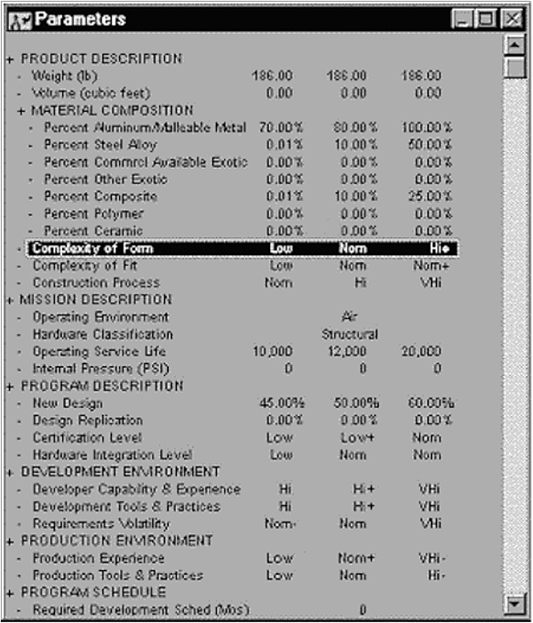
Parameters of SEER-H
SEER DFM (Design for Manufacturability) is a tool designed to assist the engineer produce and assemble products with efficiency, in a manner designed to exploit the best practices of an organization. Two fundamental analysis steps are taken in a DFM regime: the gross and detailed trade off analysis.
Gross analysis involves product design decisions, and also fundamental process and tooling decisions. Factors that influence gross analysis include the quantity of the planned product, the rate at which it will need to be produced, and the investment required. There are also machinery, assembly and setup costs to contend with.
Detailed analysis takes place once many of the primary production parameters, such as design and basic processes, have been fixed. Factors that can be adjusted for and balanced at the detailed level include tolerances, the proportion of surface finishes, secondary machining options and the age and degree of process.
SEER DFM integrates the following models:
- Machining (turning, boring milling, shaping, chemical milling, grinding…): The model explores the tradeoffs from starting with raw stock vs. sand or investment casting, etc. The material may also be varied. Tooling, setup and other costs hinge on these choices.
- Sheet metal fabrication (presses, shears, die press).
- Mechanical assembly (spot welding, bolting, bracing).
- Electrical assembly (PC board assembly, parts preparation, soldering & wave soldering, fasteners).
- Injection molding: Parameters include weight, cycle time, and cavities in the mould.
- SEER DFM performs the analysis from standard work measurements (standard times).
Reference cases
Index of cases
1. Byrne vs van Tienhoven, (1880)
2. Cahill vs Carbolic Smoke Ball Co., (1893)
3. D. & C. Builders Ltd vs Rees, (1965)
4. Dickinson vs Dodds, (1876)
5. Felthouse vs Bindley, (1862)
6. Fisher vs Bell, (1961)
7. Hadley vs Baxendale, (1854)
8. Hedley Byrne & Co. Ltd vs Heller & Partners Ltd, (1963)
9. Hyde vs Wrench, (1840)
10. Pharmaceutical Society of Great Britain vs Boots Cash Chemists(Southern) Ltd, (1953)
11. Roscorla vs Thomas, (1842)
12. Stevenson vs McLean, (1880)
13. Victoria Laundry Ltd vs Newman Industries Ltd, (1949).
14. March Construction Limited -v Christchurch City Council, (1994)
15. Blackpool & Fylde Aero Club v Blackpool Borough Council, (1990)
16. The Queen in Right of Ontario v Ron Engineering, (1981)
17. Ben Bruinsma v Chatham, (1985)
18. Megatech Contracting Ltd v Municipality of Ottawa-Carleton, (1989)
19. Chinook Aggregates Ltd v District of Abbotsford, (1990)
20. Davis Contractors v Fareham UDC, (1956)
D.1 Byrne v. Van Tienhoven (1880), 5 C.P.D. 344
On 1 October the defendants in Cardiff posted a letter to the plaintiffs in New York offering to sell them tin plate. On 8 October the defendants wrote, revoking their offer. On 11 October the plaintiffs received the defendants’ offer and immediately telegraphed their acceptance. On 15 October the plaintiffs confirmed their acceptance by letter. On 20 October the defendants’ letter of revocation reached the plaintiffs who had by this time entered into a contract to resell the tin plate. Held – (a) that revocation of an offer is not effective until it is communicated to the offeree, (b) the mere posting of a letter of revocation is not communication to the person to whom it is sent. The rule is not, therefore, the same as that for acceptance of an offer. Thus the defendants were bound by a contract which came into being on 11 October.
D.2 Carlill v. Carbolic Smoke Ball Co., (1893) 1 Q.B. 256
The defendants were proprietors of a medical preparation called ‘The Carbolic Smoke Ball’. They placed advertisements in various newspapers in which they offered to pay £100 to any person who contracted influenza after using the ball three times a day for two weeks. They added that they had deposited £1000 at the Alliance Bank, Regent Street, “to show our sincerity in the matter”. The plaintiff, a lady, used the ball as advertised and was attacked by influenza during the course of treatment – which in her case extended from 20 November 1891 to 17 January, 1892.
She now sued for £100 and the following matters arose out of the various defenses raised by the company. (a) It was suggested that the offer was too vague since no time limit was stipulated in which the user was to contract influenza. The court said that it must surely have been the intention that the ball would protect its user during the period of its use, and since this covered the present case it was not necessary to go further.(b) The suggestion was made that the matter was an advertising ‘puff,’ and that there was no intention to create legal relations. Here the court took the view that the deposit of £1000 was clear evidence of an intention to pay claims. (c) It was further suggested that this was an attempt to contract with the whole world and that this was impossible in English law. The court took the view that the advertisement was an offer to the whole world and that, by analogy with the reward cases, it was possible to make an offer of this kind. (d) The company also claimed that the plaintiff had not supplied any consideration, but the court took the view that using this inhalant three times a day for two weeks or more was sufficient consideration. It was not necessary to consider its adequacy. (e) Finally the defendants suggested that there had been no communication of acceptance but here the court, looking at the reward cases, stated that in contracts of this kind acceptance may be by conduct.
D.3 D. & C. Builders Ltd v. P@, (1965) 3 A-11 E.R. 837
D. & C. Builders, a small company, did work for Rees for which he owed £482 13s. ld. There was, at first, no dispute as to the work done but Rees did not pay. In October, 1964, the plaintiffs wrote for the money and received no reply. On 13 November, 1964, the wife of Rees (who was then ill) telephoned the plaintiffs, complained about the work, and said, “My husband will offer you £300 in settlement that is all you will get. It is to be in satisfaction.” D. & C. Builders, being in desperate straits and faced with bankruptcy without the money, offered to take the £300 and allow a year to Rees to find the balance. Mrs. Rees replied: “No, we will never have enough money to pay the balance. £300 is better than nothing.” The plaintiffs then said: “We have no choice but to accept.” Mrs. Rees gave the plaintiffs a check and insisted on a receipt “in completion of the account”.
The plaintiffs, being worried, brought an action for the balance. The defense was bad workmanship and also that there was a binding settlement. The question of settlement was tried as a preliminary issue and the judge, following Goddards v. O’Brien, (1880) 9 Q.B.D.33, decided that a check for a smaller amount was a good discharge of the debt, this being the generally accepted view of the law since that date. On appeal it was held (per The Master of the Rolls, Lord Denning) that Goddards v. O’Brien was wrongly decided. A smaller sum in cash could be no settlement of a larger sum and “no sensible distinction could be drawn between the payment of a lesser sum by cash and the payment of it by check.”
In the course of his judgment Lord Denning said of Hightrees: “It is worth noting that the principle may be applied, not only so as to suspend strict legal rights, but also so as to preclude the enforcement of them. This principle has been applied to cases where a creditor agrees to accept a lesser sum, in discharge of a greater. So much so that we can now say that, when a creditor and a debtor enter on a course of negotiation, which leads the debtor to suppose that, on payment of the lesser sum, the creditor will not enforce payment of the balance, and on the faith thereof the debtor pays the lesser sum, and the creditor accepts it as satisfaction: then the creditor will not be allowed to enforce payment of the balance when it would be inequitable to do so…. But be is not bound unless there has been truly an accord between them.” In the present case there was no true accord. “The debtor’s wife had held the creditors to ransom, and there was no reason in law or Equity why the plaintiffs should not enforce the full amount of debt.
D.4 Dickinson v. Dodds (1876), 2 Ch. D. 463
The defendant offered to sell certain houses by letter stating, “This offer to be left over until Friday, 9 a.m”. On Thursday afternoon the plaintiff was informed by a Mr. Berry that the defendant had been negotiating a sale of the property with one Allan. On Thursday evening the plaintiff left a letter of acceptance at the house where the defendant was staying. This letter was never delivered to the defendant. On Friday morning at 7 a.m. Berry, acting as the plaintiff’s agent, handed the defendant a duplicate letter of acceptance explaining it to him. However, on the Thursday the defendant had entered into a contract to sell the property to Allan.
Held – Since there was no consideration for the promise to keep the offer open, the defendant was free to revoke his offer at any time. Furthermore, Berry’s communication of the dealings with Allan indicated that Dodds was no longer minded to sell the property to the plaintiff and was, in effect, a communication of Dodds’ revocation. There was therefore no binding contract between the parties.
D.5 Felthouse v. Bindley (1862), 11 C.B.(N.S.) 869
The plaintiff had been engaged in negotiation with his nephew John regarding the purchase of John’s horse, and there had been some misunderstanding as to the price. Eventually the plaintiff wrote to his nephew as follows: “If I hear no more about him, I consider the horse is mine at £30 15s.” The nephew did not reply but, wishing to sell the horse to his uncle, he told the defendant, an auctioneer who was selling farm stock for him, not to sell the horse as it had already been sold. The auctioneer inadvertently put the horse up with the rest of the stock and sold it. The plaintiff now sued the auctioneer in conversion, the basis of the claim being that he had made a contract with his nephew and the property in the animal was vested in him (the uncle) at the time of the sale.
Held – The plaintiff’s action failed. Although the nephew intended to sell the horse to his uncle, he had not communicated that intention. There was, therefore, no contract between the parties, and the property in the horse was not vested in the plaintiff at the time of the auction sale.
D.6 Fisher vs Bell (1961)
In Fisher v. Bell (1961), a criminal case, the shopkeeper displayed a flicknife in the shop window. He was charged with offering an offensive weapon for sale, and acquitted, because the display was only an invitation to treat. (The Restriction of Offensive Weapons Act 1959 was amended immediately after this to cover the displays of weapons with a view to sale.)
D.7 Hadley v. Baxendale (1854), 9 Exch. – 41
The plaintiff was a miller at Gloucester. The drive shaft of the mill being broken, the plaintiff engaged the defendant, a carrier, to take it to the makers at Greenwich so that they might use it in making a new one. The defendant delayed delivery of the shaft beyond a reasonable time, so that the mill was idle for much longer time than should have been necessary. The plaintiff now sued in respect of loss of profits during the period of additional delay.
The court decided that there were only two possible grounds on which the plaintiff could succeed – (i) that in the usual course of things the work of the mill would cease altogether for want of the shaft. This the court rejected because, to take only one reasonable possibility, the plaintiff might have had a spare. (ii) That the special circumstances were fully explained, so that the defendant was made aware of the possible loss. The evidence showed that there had been no such explanation. In fact the only information given to the defendant was that the article to be carried was the broken shaft of a mill, and that the plaintiff was the miller of that mill. Held – that the plaintiff’s claim failed, the damage being too remote.
D.8 Hedley Byrne & Co. Ltd v. Heller & Partners Ltd, (1963) 2 All E.R. 575
The appellants were advertising agents and the respondents were bankers. The appellants had a client called Easipower Ltd, who was customers of the respondents. The appellants had contracted to place orders for advertising Easipower’s products on television and in newspapers, and since this involved giving Easipower credit, they asked the respondents, who were Easipower’s bankers, for a reference as to the creditworthiness of Easipower. Hellers replied ‘without responsibility on the part of the bank or its officials’ that “Easipower is a respectably constituted company, considered good for its ordinary business engagements. Your figures are larger than we are accustomed to see”.
Bankers normally use careful terms when giving these references, but Heller’s language was so guarded that only a very suspicious person might have appreciated that he was being warned not to give credit to the extent of £100,000. In fact Heller’s were trying to alert the plaintiffs because Easipower had an overdraft with Hellers, which Hellers knew they were about to call in and that Easipower might have difficulty in meeting the payment. One week after the reference was given Hellers began to press Easipower to reduce their overdraft.
Relying on this reply, the appellants placed orders for advertising time and space for Easipower Ltd, and the appellants assumed personal responsibility for payment to the television and newspaper companies concerned. Easipower Ltd went into liquidation, and the appellants lost over £17,000 on the advertising contracts. The appellants sued the respondents for the amount of the loss, alleging that the respondents had not informed themselves sufficiently about Easipower Ltd before writing the statement, and were therefore liable in negligence.
Held – In the present case the respondents’ disclaimer was adequate to exclude the assumption by them of the legal duty of care, but, in the absence of the disclaimer, the circumstances would have given rise to a duty of care in spite of the absence of a contract or fiduciary relationship. The dissenting judgment of Denning, L.J., in Candler v. Crane, Christmas 1951, was approved, and the majority judgment in that case was disapproved.
D.9 Hyde v. Wrench (1840), 3 Beav. 334
The defendant offered to sell his farm, for £1000. The plaintiff’s agent made an offer of £950 and the defendant asked for a few days for consideration. After this the defendant wrote, saying he could not accept it, whereupon the plaintiff wrote purporting to accept the offer of £1000. The defendant did not consider himself bound, and the plaintiff sued for specific performance.
Held – The plaintiff could not enforce this ‘acceptance’ because his counter offer of £950 was an implied rejection of the original offer to sell at £1000.
D.10 Pharmaceutical Society of Great Britain v. Boots Cash Chemists (Southern) Ltd, (1953) 1 Q.B. 401
The defendants’ branch at Edgeware was adapted to the self-service system. Customers selected their purchases from shelves on which the goods were displayed and put them into a wire basket supplied by the defendants. They then took them to the cash desk where they paid the price. One section of shelves was set out with drugs that were included in the Poisons List referred to in Sect. 17 of the Pharmacy and Poisons Act, 1933, though they were not dangerous drugs and did not require a doctor’s prescription. Section 18 of the Act requires that the sale of such drugs shall take place in the presence of a qualified pharmacist. Every sale of the drugs on the Poison List was supervised at the cash desk by a qualified pharmacist, who had authority to prevent customers taking goods out of the shop if he thought fit. One of the duties of the society was to enforce the provisions of the Act, and the action was brought because the plaintiffs claimed that the defendants were infringing Sect. 18.
Held – The display of goods in this way did not constitute an offer. The contract of sale was not made when a customer selected goods from the shelves, but when the company’s servant at the cash desk accepted the offer to buy what had been chosen. There was, therefore, supervision in the sense required by the Act at the appropriate moment of time.
D.11 Roscorla v. Thomas (1842), 3 Q.B. 234
The plaintiff bought a horse from the defendant and, after the sale had been completed, gave an undertaking that the horse was sound and free from vice. The horse was, in fact, a vicious horse, and the plaintiff sued on the express warranty which he alleged had been given to him.
Held – If the warranty had been given at the time of the sale it would have been supported by consideration and therefore actionable, but since it had been given after the sale had taken place, the consideration for the warranty was past, and no action could be brought upon it. There were no implied warranties in the contract of sale so that the plaintiff, having failed to show that the express warranty was enforceable, had no other cause of action.
D.12 Stevenson v. McLean (1880), 5 Q.B.D. 346
On Saturday the defendant offered to sell to the plaintiffs a quantity of iron at 40s. net cash per ton open till Monday (close of business). On Monday the plaintiffs telegraphed, asking whether the defendant would accept 40s. for delivery over two months or, if not, what was the longest limit the defendant would give. The plaintiffs did not necessarily want to take delivery of the goods at once and pay for it. They would have liked to have been able to ask for delivery and pay from time to time over two months as they themselves found buyers for quantities of the iron.
The defendant received the telegram at 10.01 a.m. but did not reply, so the plaintiffs, by telegram sent at 1.34 p.m., accepted the defendant’s original offer. The defendant had already sold the iron to a third party, and informed the plaintiffs of this by a telegram dispatched at 1.25 p.m. arriving at 1.46 pm. The plaintiffs had therefore accepted the offer before the defendant’s revocation had been communicated to them. If, however, the plaintiffs’ first telegram constituted a counter offer, then it would amount to a rejection of the defendant’s original offer.
Held – The plaintiffs’ first telegram was not a counter offer, but a ‘mere enquiry’ for different terms which did not amount to a rejection of the defendant’s original offer, so that the offer was still open when the plaintiffs accepted it. (Note: the defendants offer was not revoked merely by the sale of the iron to another person).
D.13 Victoria Laundry Ltd v. Newman Industries Ltd, (1949), All E.R. 997.
Loss of profits for non-delivery or delayed delivery are recoverable if foreseeable as a consequence of the breach. Thus in Victoria Laundry Ltd v. Newman Industries Ltd, (1949) 1 All E.R. 997, the defendants agreed to deliver a new boiler to the plaintiffs by a certain date but failed to do so with the result that the plaintiffs lost (a) normal business profits during the period of delay, and (b) profits from dyeing contracts which were offered to them during the period.
It was held that (a) but not (b) were recoverable as damages. This decision follows and confirmed Hedley Byrne & Co – see 8 above.
D.14 March Construction Limited v Christchurch City Council (High Court. 25.3 94).
This is a salutary reminder that bidders need to ensure that tenders are accurate.
March submitted a tender for construction to CCC. The tender contained a miscalculation in a unit price, so that the tender price was $301,631 too low. The tender was accepted and a contract in form NZS 3901:1987 signed. March completed the work- and then sued CCC for damages of $301.631.
The loss was caused by March’s miscalculation. Section 6 (1) (c) of the Contractual Remedies Act 1977 provides that the Court will not grant relief to a party if that party is obliged by a term of its contract to bear the burden of any risk. NZS 3910 provides: “Each tenderer shall be deemed to have inspected the site, examined the tender documents and any other information supplied in writing and shall have satisfied themselves as far as it is practicable for an experienced contractor before tendering as to the correctness and sufficiency of this tender for the contract works and for the price as stated in this tender”. As the contract required March to accept responsibility for the mistakes, it could not claim relief against CCC.
March also argued that CCC was liable because it failed to alert March to its own mistake and so induced March to enter the contract. This argument failed because: (a) silence is not a misrepresentation unless there is a duty to disclose and CCC had no such duty, and (b) CCC’s silence did not induce March to enter the contract. The tender was an offer which remained open until accepted. The ‘silence’ occurred after the offer was made, and therefore could not have induced the offer.
It was held March had no cause of action against CCC, and had to bear the cost of its own mistake.
D.15 Blackpool & Fylde Aero Club v Blackpool Borough Council [1990] 1 WLR 1195
A local authority put an airport concession to operate pleasure flights up to tender. They sent tender documents to the previous concessionaire and six other parties. The form of tender stated that the Council “do not bind themselves to accept all or any part of any tender. No tender which is received after the last date and time specified shall be admitted for consideration.” The plaintiffs submitted a tender within time, but the Council’s staff failed to empty the letterbox when they should have and as a result the plaintiff’s tender came to their attention too late. A tender was accepted that was lower than the plaintiffs’ tender. The plaintiffs sued.
Held – On the issue of liability it was found that the express request for tenders by the Council gave rise to an implied obligation on them to perform the service of considering all tenders that were properly submitted.
D.16 The Queen in Right of Ontario v Ron Engineering (1981) 119 DLR (3d) 267 [Supreme Ct of Canada]
A contractor submitted a $2.7m tender to construct some works. Immediately after the opening of the tenders, the contractor discovered that it had made a disastrous error in formulating its bid. It had omitted approximately $750,000 to cover the work to be done by the contractor’s own forces as opposed to subcontractors. The contractor, within 72 minutes of tender opening, told the owner about the error. The owner, however, went on to accept the tender and insisted that the contractor sign the agreement at the tendered sum. The contractor refused to do so and also attempted to recover its tender deposit of $150,000.
The court in this case held that an express provision in the contract documents put out to tender prevented all tenders from being revoked for 60 days. In their view, the submission of the tender created a contract which obliged the contractor not to withdraw its tender.
Ron Engineering has now been accepted as settled law in Canada, at least, where it is now impossible to withdraw a tender if it is expressed to be irrevocable for a stipulated period.
D.17 Ben Bruinsma v Chatham (1985) 11 CLR 37 [Ontario High Court]
All tenders to perform work on City soccer fields exceeded the City’s budget. The City decided, before contract award, to delete certain items of work. After that deletion the plaintiff’s tender was no longer the lowest and the contract was awarded to another company. It was held that the City was obliged to accept or reject the tenders as they stood. If the prices were too high, it was suggested that the City’s only option was to reject all tenders and call for new tenders for the reduced work.
Note – it has been suggested that the City could not have solved its problem by awarding the contract and then deleting part of the work. To do so would risk breaching the Fair Trading Act, if it was shown that this was the City’s intention. If, however, the City had in good faith awarded the contract and then later deleted part of the work it would probably be in the clear legally.
D.18 Megatech Contracting Ltd v Municipality of Ottawa-Carleton [1989] 68 O.R. (2d) 503 [Ontario HC]
Instructions to tenderers required tenderers to supply details of their proposed subcontractors. The lowest tender was accepted. That tender did not include the names of proposed subcontractors. The second lowest tenderer complained, arguing that the Council had acted improperly. It said that the naming of subcontractors was an important and fundamental aspect of the tendering process in that it was intended to prevent ‘bid shopping’. It said that the lowest tender should have been rejected as invalid.
The Court held that the discretionary provisions in the instructions to tenderers combined with the fact that the price was significantly lower and the tender complied substantially with the tender document requirements made the awarding of the contracts entirely proper. The employer’s actions were said not to have been arbitrary. They did not, at any point, breach the evaluation process set out in the tender specifications it distributed. The Court laid considerable emphasis on provisions in the instructions to tenderers that “the Corporation reserves the right to reject any or all tenders or to accept any tender should it be deemed in the interest of the Corporation so to do…” and that tenders ‘that contain irregularities of any kind may be rejected as informal’. Without these provisions the result may well have been different.
D.19 Chinook Aggregates Ltd v District of Abbotsford[1990] 1 W.W.R 624 [British Columbia CA]
Tenders were called for a gravel crushing contract. The instructions to tenderers said that “the lowest or any tender will not necessarily be accepted.” The Council, in fact, had a policy on preferring bids from local contractors provided those bids were within 10% of the lowest bid. This policy was not disclosed to tenderers. The lowest tenderer complained after a local contractor was awarded the contract. The Court held that the Council had acted wrongly. It was said to be in breach of a duty to treat all bidders fairly and not to give any of them an unfair advantage over the others.
D.20 Davis Contractors v Fareham UDC [1 956] 2 All ER 145.
The contractor had agreed for a lump sum to build a number of houses in 8 months. It said in a letter that the tender was “subject to adequate supplies of material and labor being available as and when required to carry out the work within the time specified”.
The House of Lords held that the letter was not, so far as this sentence was concerned, incorporated in the later formal contract signed by the parties. The Court pointed out the extreme difficulty there would have been of defining the precise content and effect of the tag had it formed part of the contract. They were of the view that if it had been part of the contract it would have meant only that the contractor would be entitled to an extension of time for any difficulty in obtaining extra labor, not extra payment.

Professional Certificate of Competency in Advanced TCP/IP-Based Industrial Networking
Designed for engineers and technicians who need practical knowledge in…Read more
Professional Certificate of Competency in Allen Bradley Controllogix / Logix5000 PLC Platforms
Designed for engineers and technicians who need practical knowledge in…Read more
Professional Certificate of Competency in Arc Flash Protection
Designed for engineers and technicians who work in the electrical…Read more
Professional Certificate of Competency in Chemical Engineering and Plant Design
Designed for engineers and technicians who need practical knowledge in…Read more
Professional Certificate of Competency in Circuit Breakers, Switchgear and Power Transformers
Designed for engineers and technicians who need practical knowledge regarding…Read more
Professional Certificate of Competency in Control Valve Sizing, Selection and Maintenance
Designed for engineers and technicians who need a solid understanding…Read more
Professional Certificate of Competency in Electrical Power System Fundamentals for Non Electrical Engineers
Designed for engineers and technicians who need to understand the…Read more
Professional Certificate of Competency in Electrical Power System Protection
Designed for engineers and technicians who need practical skills and…Read more")
Professional Certificate of Competency in Electrical Wiring Standards: AS/NZS 3000:2018 (Australia and New Zealand Only)
This professional development course is designed for engineers and technicians…Read more
Professional Certificate of Competency in Fundamental E & I Engineering for Oil and Gas Facilities
Designed for engineers and technicians who need to update their…Read more
Professional Certificate of Competency in Gas Turbine Engineering
Designed for engineers and technicians who need practical skills in…Read more
Professional Certificate of Competency in Hazardous Areas and Intrinsic Safety For Engineers and Technicians
Designed for engineers and technicians who need to understand the…Read more")
Professional Certificate of Competency in Heating, Ventilation and Air-Conditioning (HVAC)
Designed for engineers and technicians from a wide range of…Read more
Professional Certificate of Competency in IEC 61850 Based Substation Automation
Designed for engineers and technicians who need to understand the…Read more
Professional Certificate of Competency in Industrial Data Communications
Designed for engineers and technicians who need to understand how…Read more
Professional Certificate of Competency in Instrumentation, Automation and Process Control
Designed for engineers and technicians who need to gain practical…Read more
Professional Certificate of Competency in Machine Learning and Artificial Intelligence
This professional development course is designed for engineers and technicians…Read more
Professional Certificate of Competency in Mechanical Engineering
This professional development course is designed for engineers and technicians…Read more
Professional Certificate of Competency in Onshore and Offshore Pipeline Systems
Designed for engineers and technicians who need to gain an…Read more
Professional Certificate of Competency in Power Distribution
designed for engineers and technicians who need to gain a…Read more
Professional Certificate of Competency in Practical Machine Learning Using Python for Engineers and Technicians
Designed to use Python Programming to work with machine learning…Read more
Professional Certificate of Competency in Practical Python for Engineers and Technicians
Designed for engineers and technicians who need to understand the…Read more & SCADA Systems")
Professional Certificate of Competency in Programmable Logic Controllers (PLCs) & SCADA Systems
Designed for engineers and technicians who need to get practical…Read more
Professional Certificate of Competency in Project Management for Engineers & Technicians
This professional development course is designed for engineers and technicians…Read more
Professional Certificate of Competency in Safety Instrumentation Systems for Process Industries
Professional development course designed for engineers and technicians who want…Read more
Professional Certificate of Competency in Sewage and Effluent Treatment Technologies
Designed for engineers and technicians who need practical skills and…Read more
Professional Certificate of Competency in Structural Design for Non Structural Engineers
Professional development course designed for engineers and technicians who need…Read more")
Professional Certificate of Competency in Substation Design (Main Equipment)
Professional development course is designed for engineers and technicians who…Read more")
Professional Certificate of Competency in Substation Design (Control, Protection and Facility Planning)
Designed for engineers and technicians who need to gain practical…Read more
Professional Certificate of Competency in the Fundamentals of Process Plant Layout & Piping Design
Professional development course is designed for engineers and technicians who…Read more
Professional Certificate of Competency in Practical Mechanical Sealing
This professional development course is designed for engineers and technicians…Read more
Professional Certificate of Competency in Road Construction
This professional development course is designed for engineers and technicians…Read more
Professional Certificate of Competency in Specification and Technical Writing
Master the art of writing clear, accurate, and professional technical…Read more
Professional Certificate of Competency in Hydraulics and Pneumatics
Overview of all aspects related to the construction, design, operation,…Read more
Professional Certificate of Competency in Big Data and Analytics in Electricity Grids
This course explores the use of big data & data…Read more
Professional Certificate of Competency in Renewable Energy Systems
This course covers various renewable energy systems that are popular…Read more
Professional Certificate of Competency in Smart Grids
A smart grid is an electricity network that uses digital…Read more
Professional Certificate of Competency in Hydrogen Energy – Production, Delivery, Storage and Use
Hydrogen energy short course designed for engineers and professionals interested…Read more")
Professional Certificate of Competency in Building Information Modelling (BIM)
This professional development course is covering practical aspects of using…Read more
Professional Certificate of Competency in Industrial Internet of Things
Internet of Things (IoT) is the most sort after technology…Read more