This introductory manual is designed for those with minimal background who seek a basic understanding of the practical aspects of mechanical engineering.
IDC Technologies Pty Ltd
PO Box 1093, West Perth, Western Australia 6872
Offices in Australia, New Zealand, Singapore, United Kingdom, Ireland, Malaysia, Poland, United States of America, Canada, South Africa and India
All rights to this publication, associated software and workshop are reserved. No part of this publication may be reproduced, stored in a retrieval system or transmitted in any form or by any means electronic, mechanical, photocopying, recording or otherwise without the prior written permission of the publisher. All enquiries should be made to the publisher at the address above.
ISBN: 978-1-921007-07-1
Disclaimer
Whilst all reasonable care has been taken to ensure that the descriptions, opinions, programs, listings, software and diagrams are accurate and workable, IDC Technologies do not accept any legal responsibility or liability to any person, organization or other entity for any direct loss, consequential loss or damage, however caused, that may be suffered as a result of the use of this publication or the associated workshop and software.
In case of any uncertainty, we recommend that you contact IDC Technologies for clarification or assistance.
Trademarks
All logos and trademarks belong to, and are copyrighted to, their companies respectively.
Acknowledgements
IDC Technologies expresses its sincere thanks to all those engineers and technicians on our training workshops who freely made available their expertise in preparing this manual.
Contents
1 Basics of Mechanical Engineering 1
1.1 Introduction 1
1.2 Basic concepts 2
1.3 Units of engineering quantities 5
1.4 Friction 6
1.5 Summary 9
2 Mechanical Drawings 11
A Types of lines and letters used in drawings 11
2.1 Types of lines 11
2.2 Lettering in the drawings 14
2.3 Summary for Section A 15
B Projections 15
2.4 What is projection? 15
2.5 Pictorial projections 17
2.6 Concept of cutting plane and sectional views 18
2.7 Summary of Section B 23
C Dimensioning 23
2.8 Different systems of dimensioning 23
2.9 Dimensioning practices 23
2.10 Summary of Section C 25
D Assembly drawings 25
2.11 Summary of Section D 26
E Welded joints 26
2.12 Types of welded joints 27
2.13 Summary of Section E 29
F Bolt, nut and screw fasteners 29
2.14 Introduction 29
2.15 Summary of Section F 31
G Keys, keyways and keyed assemblies 31
2.16 Types of keys 32
2.17 Summary of Section G 33
H Tolerance, limits and fits 34
2.18 Concept of tolerance 34
2.19 Concept of limits 35
2.20 Concept of fit 36
2.21 Summary of Section H 37
I The role of CAD and CAM 38
2.22 Use of computers for preparation of drawings 38
2.23 CAD software 38
2.24 Computer Aided Manufacturing (CAM) 39
2.25 Summary of Section I 39
J Office practice 39
2.26 Drawing number and part name 39
2.27 Summary of Section J 40
3 Engineering Materials 41
3.1 Mechanical properties of materials 41
3.2 Processing of metals and alloys 43
3.3 Stress and strain in metals 46
3.4 Normal stress and shear stress 48
3.5 Tensile and hardness testing 48
3.6 Stress and strain diagram 52
3.7 Alloy production and properties 55
3.8 Fracture of metals 60
3.9 Corrosion types and control 64
3.10 Summary 65
4 Mechanical Design 67
4.1 Introduction 67
4.2 Codes and standards 70
4.3 Design considerations 70
4.4 Factory of safety 76
4.5 Mechanical components 77
4.6 Fasteners/screwed joints 105
4.7 Fastener failure 111
4.8 Compression members 115
4.9 Summary 120
5 Mechanical Engineering Codes and Standards 123
5.1 Need for standardization 124
5.2 Overview of standards 124
5.3 Benefits of standardization 125
5.4 Mechanical engineering standards 126
5.5 ISO 9000/1 126
5.6 Six-sigma 128
5.7 Summary 129
6 Manufacturing 131
6.1 Foundry processing 131
6.2 Heat treatment 134
6.3 Hot working of metals 135
6.4 Cold working of metals 137
6.5 Pressing 139
6.6 Numerical control 142
6.7 Sawing 146
6.8 Broaching 146
6.9 Shapers and shaping 147
6.10 Welding 147
6.11 Brazing 148
6.12 Computer-aided manufacturing 149
6.13 Manufacturing processes in oil and gas industry 150
6.14 Summary 150
7 Mechanical Automation 151
7.1 Sensors and actuators 151
7.2 Differential transformers 158
7.3 Velocity and motion 162
7.4 Fluid pressure measurement 164
7.5 Liquid flow measurement 165
7.6 Liquid level measurement 167
7.7 Temperature measurement 168
7.8 Light sensors 169
7.9 Selection of sensors 170
7.10 Pneumatics and hydraulics 170
7.11 Control valves 172
7.12 Cylinders 176
7.13 Electrical actuation 178
7.14 Electrical drives 180
7.15 Electrical machines 181
7.16 Gear motors 186
7.17 Control systems 187
7.18 Summary 192
8 Fluid Engineering 195
8.1 Pumps 195
8.2 Compressors 207
8.3 Turbines 211
8.4 Flow in pipes 217
8.5 Thermodynamics 223
8.6 Reversibility 228
8.7 Summary 229
9 Maintenance of Machinery 231
9.1 The need for maintenance 231
9.2 Types of maintenance 232
9.3 Maintenance strategies 233
9.4 Failure 234
9.5 How to select your maintenance plan 235
9.6 Predictive maintenance techniques 236
9.7 Summary 244
10 Theory of Heat Transfer 245
10.1 Heat basics 245
10.2 Heat transfer 247
10.3 Laws of Thermodynamics 249
10.4 Thermal cycles 251
10.5 Heat cycles 258
10.6 Heat pumps 261
10.7 Air conditioning 263
10.8 Summary 264
Exercises 265
Answers 309
Mechanical Engineering, as its name suggests, deals with the mechanics of operation of mechanical systems. This is the branch of engineering which includes design, analysis, testing, manufacturing and maintenance of mechanical systems. The mechanical engineer may design a component, a machine, a system or a process. Mechanical engineers will analyze their design using the principles of motion, energy, and force to ensure the product functions safely, efficiently, reliably, and can be manufactured at a competitive cost.
Learning objectives
Basic concepts
Units for engineering quantities
Friction and its importance
1.1 Introduction
Mechanical engineering plays a dominant role in enhancing safety, economic vitality, enjoyment and overall quality of life throughout the world. Mechanical engineers are concerned with the principles of force, energy and motion.
Mechanical engineering is a diverse subject that derives its breadth from the need to design and manufacture everything from small individual parts and devices (e.g. microscale sensors and inkjet printer nozzles) to large systems (e.g. spacecraft and machine tools). The role of a mechanical engineer is to take a product from an idea to the marketplace. In order to accomplish this, a broad range of skills are needed. Since these skills are required for virtually everything that is made, mechanical engineering is perhaps the broadest and most diverse of engineering disciplines.
Mechanical engineers play a central role in such industries as automotive (from the car chassis to its every subsystem—engine, transmission, sensors); aerospace (airplanes, aircraft engines, control systems for airplanes and spacecraft); biotechnology (implants, prosthetic devices, fluidic systems for pharmaceutical industries); computers and electronics (disk drives, printers, cooling systems, semiconductor tools); microelectromechanical systems (MEMS) (sensors, actuators, micropower generation); energy conversion (gas turbines, wind turbines, solar energy, fuel cells); environmental control (HVAC, air-conditioning, refrigeration, compressors); automation (robots, data and image acquisition, recognition, control) and manufacturing (machining, machine tools, prototyping, micro fabrication).
The main areas of study in this branch are:
Materials
Solid and fluid mechanics
Thermodynamics
Heat transfer
Control, instrumentation
Specialized mechanical engineering subjects include biomechanics, cartilage-tissue engineering, energy conversion, laser-assisted materials processing, combustion, MEMS, micro fluidic devices, fracture mechanics, nanomechanics, mechanisms, micropower generation, tribology (friction and wear) and vibrations.
1.2 Basic concepts
1.2.1 Force
A foundation concepts in physics, a force may be thought of as any influence which tends to change the motion of an object. A force can be described as the push or pull upon an object resulting from the object’s interaction with another object. Whenever there is an interaction between two objects, there is a force upon each of the objects. When the interaction ceases, the two objects no longer experience the force. Forces only exist as a result of an interaction.
There are four fundamental forces in the universe: the gravity force, the nuclear weak force, the electromagnetic force, and the nuclear strong force in ascending order of strength. In mechanics, forces are seen as the causes of linear motion, whereas the cause of rotational motion is called a torque. The action of forces in causing motion is described by Newton’s Laws.
Force is a quantity which is measured using the standard metric unit called the Newton. A Newton is abbreviated by a “N”. To say “10.0 N” means 10 Newtons of force. One Newton is the amount of force required to give a 1 kg mass an acceleration of 1 m/s2.
Force = mass x acceleration
F = m x a = 1 kg x 1 m / s2
A force is a vector quantity—it has both magnitude and direction. To fully describe the force acting upon an object, you must describe both the magnitude (size or numerical value) and the direction. Thus, 10 Newtons is not a full description of the force acting upon an object. In contrast, 10 Newtons downwards is a complete description of the force acting upon an object; both the magnitude (10 Newtons) and the direction (downwards) are given.
A torque is a special form of force that turns an axle in a given direction. It is sometimes called a rotational force. You can create a torque by pushing on a rod or lever that rotates an axle. Likewise, a torque on an axle can result in a linear force at a distance from the center of the axle.
Torque equals force multiplied by moment arm. Pushing on a rod that rotates an axle can create a torque on that axle. Likewise, a torque on an axle can result in a linear force at a radius from the center.
The relationship between torque and force is:
T = FR
or
F = T/R
where
T is the torque in newton-meters
F is the force (Newtons)
R is the radius or distance from the center to the edge (meters)
R is also sometimes called the moment arm. The force, F, is applied perpendicular to the radius, lever or moment arm.
1.2.2 Work
Work refers to an activity involving a force and movement in the direction of the force.
A work is done on an object when the force acts on it in the direction of motion or has component in the direction of motion.
In order to accomplish work on an object there must be a force exerted on the object and it must move in the direction of the force.
Work = Force x distance moved in direction of force
Work is measured in joules (J ). The formula for this is:
J = N x m
Where force is measured in Newtons and distance in meters.
For a constant force F which moves an object in a straight line from x1 to x2, the work done by the force
Work = force x (x2-x1)
Mathematically, work can be expressed by the following equation:
W = F x d x cos Θ
where F is the force, d is the displacement, and the angle (theta) is defined as the angle between the force and the displacement vector. Perhaps the most difficult aspect of the above equation is the angle “theta.” Theta is defined as the angle between the force and the displacement.
A force acts from the right on an object and it is displaced to the right. In such an instance, the force vector and the displacement vector are in the same direction. Thus, the angle between F and d is 0 degrees.
A force acts from the left on an object and it is displaced to the right. In such an instance, the force vector and the displacement vector are in the opposite direction. Thus, the angle between F and d is 180 degrees.
A force acts upward on an object as it is displaced to the right. In such an instance, the force vector and the displacement vector are at right angles to each other. Thus, the angle between F and d is 90 degrees.
For the more general case of a variable force F(x) which is a function of x, the work is still the area under the force curve, and the work expression becomes an integral.
Work is not done when there is no motion or when the force is perpendicular to the motion.
Let us apply the work equation to determine the amount of work done by the applied force in each of the three situations described below.
Diagram A Answer:
W = (100 N) x (5 m) x cos (0 degrees) = 500 J
The force and the displacement are given in the problem statement. It is said (or shown or implied) that the force and the displacement are both to the right. Since F and d are in the same direction, the angle is 0 degrees.
Diagram B Answer:
W = (100 N) x (5 m) x cos (30 degrees) = 433 J
The force and the displacement are given in the problem statement. It is said that the displacement is to the right. It shows that the force is 30 degrees above the horizontal. Thus, the angle between F and d is 30 degrees.
Diagram C Answer:
W = (147 N) x (5 m) x cos (0 degrees) = 735 J
1.2.3 Energy
Energy is the capacity for doing work. You must have energy to accomplish work – it is like the “currency” for performing work. In the process of doing work, the object which is doing the work exchanges energy with the object upon which the work is done. When the work is done on the object it gains energy. The energy acquired by the objects upon which work is done is known as mechanical energy.
Mechanical energy is the energy which is possessed by an object due to its motion or due to its position. Mechanical energy can be either kinetic energy (energy of motion) or potential energy (stored energy of position). Objects have mechanical energy if they are in motion and/or if they are at some position relative to a zero potential energy position.
Mechanical energy = Kinetic energy + Potential energy
Potential Energy PE = mass of the object x acceleration of gravity x height of the object
PE = m x g x h
g represents the acceleration of gravity (9.8 m/s/s on Earth)
Kinetic Energy is depend on two variables: the mass and the speed
The following equation is used to represent the kinetic energy (KE) of an object.
KE = 1/ 2 x m x v 2
1.2.4 Power
Power is the rate at which work is done. It is the work/time ratio. Mathematically, it is computed using the following equation.
Power = work / time = (force x displacement) / time
The standard metric unit of power is the Watt. As is implied by the equation for power, a unit of power is equivalent to a unit of work divided by a unit of time. Thus, a Watt is equivalent to a Joule/second. For historical reasons, the term ‘horsepower’ is occasionally used to describe the power delivered by a machine. One horsepower is equivalent to approximately 750 Watts.
Most machines are designed and built to do work on objects. All machines are typically described by a power rating. The power rating indicates the rate at which that machine can do work upon other objects. Thus, the power of a machine is the work/time ratio for that particular machine. The power rating relates to how rapidly the engine can accelerate the car.
1.3 Units of engineering quantities
Table 1.1 gives the most common units of engineering quantities that you will come across.
Figure 1.1 shows a representation of the linkage of basic mechanical units.
Table 1.1 Units of engineering quantities
SI units
US common
Length (L)
Meter m
Foot ft
Time (T)
Second s
Second s
Mass (M)
Kilogram kg
Slug
Velocity (L/T)
m / s
ft/s
Acceleration (L/T2 )
m/ s2
ft/ s2
Force (M L/ T2)
kg m / s2 = Newton N
slug ft/ s2 = pound lb
Work (M L2/ T2)
N m = J joule
lb ft = ft lb
Energy (M L2/ T2)
joule
ft lb
Power (M L2/ T3)
J / s = W watts
ft lb/s
Figure 1.1 Basic Mechanical units
1.4 Friction
Friction is a force that is created whenever two surfaces move or try to move across each other. Friction always opposes the motion or attempted motion of one surface across another surface. Friction is dependant on the texture of both surfaces and the amount of contact force pushing the two surfaces together.
In a machine, friction reduces the ratio of output to input. An automobile, for instance, uses one-quarter of its energy on reducing friction. Yet it is also friction in the tires that allows the car to stay on the road, and friction in the clutch that makes it possible to drive at all. From matches to machines to molecular structures, friction is one of the most significant phenomena in the physical world.
There are advantages and disadvantages of friction. Since friction is a resistance force that slows down or prevents motion, it is necessary in many applications to prevent slipping or sliding. But it can also be a nuisance because it can hinder motion and cause the need for expending energy. A good compromise is necessary to get just enough friction.
Disadvantages of friction:
makes movement difficult
machine parts get overheated
wastes energy
any device that has moving parts can wear out rapidly due to friction. Lubrication is used not only to allow parts to move easier but also to prevent them from wearing out.
The force of friction is a force that resists motion when two objects are in contact. If we look at the surfaces (Figure 1.2) of all objects, there are tiny bumps and ridges. Those microscopic peaks and valleys catch on one another when two objects are moving past each other.
Figure 1.2 Typical surface
There are two types of friction
Static
Kinetic
If we try to slide two objects past each other, a small amount of force will result in no motion. The force of friction is greater than the applied force. This is static friction. (Figure 1.3) If we apply a little more force, the object ‘breaks free’ and slides, although we still need to apply force to keeps the object sliding. This is kinetic friction (Figure 1.4). We need not apply quite as much force to keep the object sliding as we originally needed to break free from the static friction.
Figure 1.5 shows the relationship between applied force and frictional force.
Figure 1.5 Relationship between applied and frictional force
Let’s examine the relationship between these two forces and the applied force that creates them. Figure 1.5 shows static frictional force increasing to a maximum with the application of a force then dropping off sharply to a lesser value (kinetic friction) once the object starts moving. We can conclude few points from this graph such as those listed below.
Static friction:
Static friction fs is proportional to Fn (surface normal force)
It is independent of area
It reaches a maximum value (which depends on the surface materials) in preventing motion between surfaces, and then drops to the lower value of sliding friction as the object begins to move.
Kinetic friction:
Kinetic friction fk is proportional to Fn
It is also independent of area and speed of surfaces
It is always less than static friction fk < fs (meaning it’s easier to push an object once it’s moving)
Since friction is proportional to the force pressing the surfaces together (Fn)
f αFn
which means that,
f / Fn = constant
This constant is known as coefficient of friction: μ (the Greek letter ‘mu’). Thus we can write the equation as:
f = μ x Fn
Since static friction and kinetic friction are different, there is a μ for each one:
μs = coefficient of static friction
μk = coefficient of kinetic friction
Table 1.2 shows some common values of coefficients of kinetic and static friction.
Static friction fs <μs Fn
Kinetic fk = μkFn
Note that static friction is expressed as an inequality in the above equation. This is because it varies from zero to a maximum. At the maximum value, and only at the maximum value (just before the object moves), the static frictional force is exactly equal to μsFn, or
fs max = μs Fn
Coefficient of friction μ = f / Fn
Table 1.2 Some common values of coefficients of kinetic and static friction
Surfaces
µ (static) μs
µ (kinetic) μk
Steel on steel
0.74
0.57
Glass on glass
0.94
0.40
Metal on Metal (lubricated)
0.15
0.06
Ice on ice
0.10
0.03
Teflon on Teflon
0.04
0.04
Tire on concrete
1.00
0.80
Tire on wet road
0.60
0.40
Tire on snow
0.30
0.20
These values are approximate.
1.5 Summary
Mechanical Engineering deals with mechanics of operation on different systems. The various functions that fall within the scope of this branch are designing, manufacturing and maintenance. For this purpose it uses laws of physics and applies them to analyze their performance.
Friction is a force which is created when two surfaces move across each other. It plays very important role in some situations like walking, writing, etc. where you could not do without the force of friction. In some cases friction is less required, so compromise is required.
This chapter explains all the details about mechanical drawing from line work to tolerance limits. All the aspects of mechanical drawings including the quality details are covered in this chapter. To aid your understanding, we have split this chapter in to ten individual sections.
Learning objectives
To learn types of lines and letters used in a mechanical drawing
To the concepts related to mechanical drawing like dimensioning
To study about the various views used in mechanical drawings
To understand the concepts like CAD/CAM
To study the welded joints and it’s drawings
To learn about bolts, rivets, keys and other joints with their drawings.
To learn how office maintenance practices of drawings increase productivity
To learn the importance of properly recording all drawing updates
A Types of lines and letters used in drawings
A mechanical drawing will consist of lines and letters of different types. Thus, lines could be straight or curved, thick or thin, continuous or broken etc. Similarly, letters could be vertical or slant, capital or lower case, plain or decorative, etc. This chapter gives the characteristics of lines and letters used in mechanical drawings.
2.1 Types of lines
Many different types of lines are used in mechanical drawings. Important ones are given in Table 2.1.
Table 2.1 Lines used in Mechanical Engineering Drawings
Example
Application
Visible edges and outlines
A
Continuous (thick)
Visible edges and outlines
B
Continuous (thin)
Dimensions and projection lines
Hatching lines for cross sections
Leader lines
Outlines of revolved sections
Imaginary lines of intersection
C
Continuous (thin) irregular
Limits of partial views or sections (provided the line is not an axis)
D
Short dashes (thin)
Hidden outlines and edges
E
Chain (thin)
Centre lines
F
Chain (thick)
Used for surfaces which have to meet special requirements
G
Thin chain with thick line at the ends and at changes in direction, to indicate cutting planes
Cutting planes which may be in one or more parallel planes, adjacent planes or intersecting planes.
2.1.1 Continuous (thick) line
A continuous (thick) line is used to show the boundaries (external or internal) of the object which are visible in that particular view, as seen in Figure 2.1.
Figure 2.1 Thick line
2.1.2 Continuous (thin) line
A continuous (thin) line such as that in Figure 2.2 is used for most of the remaining cases such as:
Dimension line
Extension line
Hatching line
Leader line
Line of (imaginary) intersection
Other places except boundaries
Figure 2.2 Thin line
2.1.3 Continuous (thin) irregular line
This line is used to indicate the limits of partial views or sections (provided it is not an axis line) . This is drawn freehand and usually spans over short distance where the view is broken for clarity. See Figure 2.3.
Figure 2.3 Continuous (thin) irregular line
2.1.4 Dashed line
This line constitutes of only short dashes as shown in Figure 2.4 . This line is used to show the edge or the boundary of a part which is hidden behind some other surface.
Figure 2.4 Dashed line
2.1.5 Dash and dot line
This line is a chain of short thin dash and a dot. This type of line is used for centre line of an object (see Figure 2.5). In some cases a chain of (thick) dash and dot is used to indicate a surface which has to meet special requirements. But this is more of an exception than a regular practice. This line is also used to show locus of particular part.
Figure 2.5 Dash and dot line (thin or thick)
2.1.6 Chain of combination of long thick-thin line and a dot
In this chain, the ends and the bends are shown by thick lines with thin lines over rest of the chain as shown in Figure 2.6. This line is used for cutting planes. This is also very useful to show the details of a component which has multiple center lines at different places in the same plane.
Figure 2.6 Chain of thick and thin lines with a dot.
2.1.7 Chain of dash and double dots
This line is used for adjacent part which really do not form part of the assembly under study but is useful in understanding the functioning of a system as a whole. It is also used to show the extreme positions of movable parts. Thus it is related to the outline of performance of a mechanism. This type of line is very effective to display unconventional features which help understand the drawing and the actual mechanism (see Figure 2.7).
Figure 2.7 Chain of dash and double dots.
2.2 Lettering of drawings
As will be seen later, a lot of lettering is required on drawings such as dimensions, specifying cross section planes, cross references of other drawings, title block, notes, etc. A decent size, stroke, style, spacing between lines, between letters, between words, thickness of strokes and all such factors go a long way to make a drawing easy to read and understand. A legible and uniform lettering also improves the appearance of the drawing.
The size of the characters (letters and numbers) will depend upon the size of the drawing. Minimum sizes are given in Table 2.2. Higher sizes could be used based on requirements (such as highlighting a particular note or dimension to attract attention of the user).
Table 2.2
Minimum size of letters
Application
Drawing sheet size
Minimum character height
Drawing numbers, etc.
A0, A1, A2, A3
7 mm
A4
5 mm
Dimensions and notes
A0
3.5 mm
A1, A2, A3, A4
2.5mm
2.2.1 Lettering strokes
Lettering stroke is a choice of the individual and could be vertical or slanted. Similarly, it could be capital or lower case, normal or bold, etc. However, it is preferable to use the same stroke all over a drawing sheet. It is recommended to have slant strokes with a 15 degrees slope to vertical. Underlining the letters should be done only in exceptional circumstances. Also consistency in the size, shape, density, etc. over the full drawing is highly desirable. Fonts and strokes should be simple. Fancy strokes should not be used.
2.3 Summary of Section A
This section gives the characteristics of lines and letters used in mechanical drawings. Different types of lines and letters are used in the mechanical drawing. Certain conventions should be followed. Good line work and lettering makes the drawing simple and pleasing to read.
B Projections
In mechanical drawing, three views of the object are drawn to get complete idea about the shape of the object. The three views are views from top, front and side. There are two types of projection: first and third angle projection system. A pictorial view – either isometric or oblique – gives a better idea about the object.
2.4 What is projection?
A projection is a two dimensional image of a two or three dimensional object on a plane. The image of the object depends on the following three factors concerning the point of viewing (real or imaginary position of eye)
the line of viewing (the imaginary lines of sight for seeing the object)
the plane on which the object is projected and
the object by itself.
If the point of viewing is located at infinity, then all lines of viewing the various points on the object become parallel to each other and perpendicular to the plane of projection. If the object is three-dimensional (solid), the image formed is projection of visible area. This is called orthographic projection. All engineering drawings are orthographic unless specified otherwise.
Three such projections from three different view points are adequate to provide full geometric information about the object. In an engineering drawing, a projection on the paper is not simply image of the boundaries of the object on a plane but a drawing of every line, every border seen by the observer on a particular plane viewed from infinity and at a particular line-of-sight.
The three views used in engineering drawing are:
View from top projected on a horizontal plane (called the plan view)
View from front projected on a vertical plane (called the elevation/front view)
View from a side on a plane perpendicular to both the horizontal and the vertical planes (called the side view)
In engineering drawing we use the rectilinear system of coordinates with the three axes perpendicular to each other and the three planes formed by these three axes named the horizontal plane, vertical plane and side plane. The axes system is generally a right-handed axes system. The three views as mentioned above will be different for the same object if the selection of the three planes is different in each case. To avoid confusion in understanding the drawing by a third person, it is necessary to specify the quadrant where the object is located and the planes used for projection by the designer/draftsman in the preparation of drawing.
In the field of engineering drawing, two systems of projection are normally followed:
First angle projection
Third angle of projection.
These two systems are explained below.
2.4.1 First angle and third angle projections
In the First angle method of projection, the object is assumed to be placed in the first quadrant and the three views are drawn on the horizontal, vertical and side plane as mentioned above. Then, the vertical plane and the side plane are rotated by 90 degrees to form a single plane surface which shows all three views. In the same manner, in the third angle projection, the object is placed in the third quadrant, the three views are drawn and the vertical and side planes rotated by 90 degrees to form a single plane surface showing the three views.
The assumption made by the draftsman, whether first angle or third angle, is clearly recorded in the title block of the drawing. The symbols used for these two systems are given in Figures 2.8 and 2.9.
Figure 2.8 Symbol of first angle ProjectionFigure 2.9 Symbol of third angle
The three views of the object given in Figure 2.10 are shown in Figures 2.11 and 2.12 respectively.
Front view: Drawn looking straight at the front of the object.
Side view: The left side of the object is drawn toward the right side view of the object and vice versa.
Plan View: The top of the object is drawn toward the bottom view of the object and vice versa.
Figure 2.10 The objectFigure 2.11 Three views in firstFigure 2.12 Three Views of angle projection
Both first angle and third angle projections are quite popular and used widely in the industry. Figure 2.13 is an example of third angle projection.
Figure 2.13 Isometric projection and three views in third angle projectionFigure 2.14 Three views of the object shown in Figure 2.13 drawn in third angle projection
2.5 Pictorial projections
While the three view drawing can be understood by the engineers, his understanding of the object can be shown in a single pictorial view on a plane which is much easy to visualize (but difficult to draw!). There are two types of pictorial drawings:
Isometric projection
Oblique projection
2.5.1 Isometric projection
In isometric projection, the two axes are at 60 degrees to the vertical axis and the measurements along these two axes can either be scaled from measurements on actual objects or they can be actual measurements if the space permits. The isometric projection of a cube is shown below in Figure 2.15.
Figure 2.15 Isometric projection of a cube
2.5.2 Oblique projection
In this method, the two axes are at right angles to each other and the third axis is at 45 degrees to them. The oblique projection of a cube is shown in Figure 2.16.
Figure 2.16 Oblique projection
2.6 Concept of cutting plane and sectional view
The plane which cuts the object under observation, either fully or partially is called a cutting plane. This is an imaginary plane and does not have any specified dimensions. It is drawn as a thick dark line at the extremes and thin long line followed by two short lines in a chain. The cutting plane need not always be a single plane but it could consist of more planes with changing directions. It is drawn thick whenever it is changing direction. At the two extremes, two short lines with small arrow heads are drawn perpendicular to the cutting plane. These arrowheads indicate the viewing direction or the line-of-sight. The cutting planes are identified by letters A-A, B-B, etc. written near the arrow heads to distinguish one view from other on the same drawing sheet.
2.6.1 Sectional views
The views of the object drawn after cutting it by a plane are called sectional views. Sectional views are drawn to clarify the interiors or hidden details on a multi-view drawing of an object. The observer imagines that the object is cut by a plane (cutting plane) and that the part of object nearer to the observer is removed from the view exposing the interiors of the object where a cut has been taken.
The sectional view usually replaces one of the principal views (plan, front view or side view) depending upon position of cutting plane. However it is not a rule and the sectional view many times supplements the other view to give the clear idea about the external as well as the internal details of the object. Hidden lines are omitted in the sectional views to avoid the confusion between dotted lines and hatching lines. However in the portion where the object is not cut, we follow the normal convention that the hidden lines are dotted.
The spokes and the ribs of a wheel are not sectioned in the plane of the wheel even though it may cut them. (Spokes are thin wire-like elements which hold the rim and the wheel hub together whereas the ribs are the strengthening or reinforcing parts of the wheel).
It is also conventional drawing practice not to take sections on keys, key ways, nuts, bolts and other fasteners in the assembly in which they are used.
Figure 2.17 Sectional view of a wheel with hatching convention.
A separate sectional view giving the cross sectional details of the spoke, rib or key, etc. can be drawn to supplement the sectional view of wheel and hub or shaft.
Types of sectional views
Types of sectional views are as follows:
Full section view
Half section view
Rotated section view
Removed section view
Allied section view
Offset section
Partial section
Assembly section
Pictorial section
Each one of these is explained below with an illustration.
Full section view
This is the simplest type of section in which the cutting plane cuts the object in two and half the object nearer to the observer is removed. This section is very useful for the parts or assemblies which are symmetrical about the center line. This is illustrated in Figure 2.18 (a).
Half section view
In this case two cutting planes placed at 90 degrees to each other cut the object halfway through We remove one quarter of the object which is cut from the main object exposing two half surfaces of the object at 90 degrees to each other. This section is very useful and elegant way of showing the interior portion of a symmetrical object. This is shown in Figure 2.18 (b).
Figure 2.18(a) Full sectionFigure 2.18(b) Half section
Note the thick lines in Figure 2.18 (a) and dotted lines in Figure 2.18 (b) on the right half of the views showing the internal details of the object. The other half of is identical in both sectional views. Also note the hatching on the exposed cut area. It is conventional to do the hatching of such surfaces to highlight the fact that the area is a cut area. The hatching also indicates the material of the cut area. Details of hatching are given later. Further, note that other outside views are not affected while drawing a sectional view.
Rotated or revolved sectional view
This sectional view is used to show the uniform shape of object from end to end. See Figure 2.19. Here the object is a square pipe with a rectangular cavity all through. This is shown by revolving the cross section of the pipe drawn along the length itself of the pipe itself.
Removed section
This sectional view is used to show the variable shape of an object from end to end. This is shown in the lower portion of Figure 2.19. Here the object is a circular pipe in the middle portion, with different cross sections for the end portions as shown. Such parts are not uncommon in mechanical engineering.
Aligned section
These views are drawn to show the shape of features that do not align with vertical and horizontal center lines of the object (see Figure 2.19).
Here the cutting plane is aligned to pass through the holes of the flange which are located at 45 degrees to vertical and horizontal planes. Hence a vertical or horizontal cross section would not have revealed these holes.
Figure 2.19 Aligned and offset Sections
Offset sections
A little complicated situation may arise when even one aligned cutting plane may not be sufficient to show the holes or other details of the vertical or horizontal plane. For example, the lower part of the Figure 2.19 shows different holes of varying size and shape, at different vertical cutting planes. In this case the cutting plane is offset to pass through all the desired locations. Note the different shape of each hole – first and third holes are circular, second is countersunk, the fourth is drilled hole which terminates in the plate and the last is threaded drill.
Broken out sections
These sectional views are drawn to show material thickness of a hollow object. See Figure 2.20.
Partial sections
These are similar to broken out sections with the difference that they usually cover a little larger area but less than half section.
Assembly section
This section shows the arrangement and relationship of parts that make up the object.
Pictorial sections This section shows the arrangement and relationship of parts in a three-dimensional view with a quarter or half object removed.
Figure 2.20 Broken-out, pictorial and assembly sections
Hatching of sectional views
Hatching of sectioned views is done to distinguish solid portions from hollow portions.
There are different types of hatching for different purposes. Thus a sectional view of a part made of cast iron is hatched with thick lines spaced at 3 mm spacing. Different materials have different patterns of hatching (see Figure 2.21).
Slope of hatching lines should be changed by 90 degrees on adjacent parts in the assembly drawings.
Figure 2.21 Hatching pattern for different metallic materials
2.7 Summary of Section B
A projection is a two dimensional image of a two or three dimensional object on a plane. The image of the object depends on point of viewing (real or imaginary position of eye), the line of viewing (the imaginary lines of sight for seeing the object), the plane on which the object is projected and the object by itself..
Two systems of projection are first angle projection and third angle of projection. These two systems are explained in this section with examples. Isometric projection and oblique projections are pictorial presentation of object. These are also explained with example.
The plane that cuts the object under observation, either fully or partially is called a cutting plane. This is an imaginary plane. The views of the object drawn after cutting it by a plane are called sectional views. Sectional views are drawn to clarify the interiors or hidden details on a multi-view drawing of an object. Hatching of sectioned views is done to distinguish solid portions from hollow portions. Types of sectional views and types of hatching are explained
C Dimensioning
A drawing prepared by the designer is used by many departments such as tooling, manufacturing, inspection, material procurement and customer acceptance.
Thus it becomes the basic document for all departments once it is released from design department. Therefore it is important that the drawing contains all information required by these departments and there is no ambiguity at any stage. Size of the part – length, width, height, diameter, etc. has to be specified on the drawing. All dimensions required for the purpose of manufacturing and acceptance of the part or a product have to be specified. The dimension given by the designer is called the nominal dimension. Designer also has to give some allowance since no part ca be made exactly to the nominal size. The designer has also to keep in mind the assembly requirements.
2.8 Different systems of dimensioning
There are two systems of dimensioning and each industry has its own preference. The two systems are:
aligned system
unidirectional system
In the aligned method, all horizontal dimension lines are placed on the bottom side of the part and all vertical dimension lines are put on the right side of the part. Value of the size is invariably put on the top of the dimensional line. This avoids the confusion in reading the numerals 6 and 9.
In the unidirectional method, all dimension lines are placed horizontally as in aligned method but the dimensions are placed in the center of the dimension line drawn horizontal or vertical.
These two methods are supplemented by other norms for dimensioning the circular parts, drilled parts, welded parts, bolted assemblies and many other situations. The basic idea is to give clear information of size without making the drawing clumsy to read.
2.9 Dimensioning practices
All dimension lines are thin and continuous (except for the break for dimension value) placed outside the external boundary of the object. The dimension lines are bounded on both sides by small lines perpendicular to the dimension line called as projection lines. These projection lines are drawn so they do not touch the boundary line of the part. Arrowheads are put on either ends of dimension line to specify the extent of part covered by the dimension. Arrowheads are drawn approximately triangular in shape. The size and shape of the arrows is kept uniform all over the drawing in one sheet. The units for the dimensions are specified in the title block and only one system, either British Imperial or metric, is followed all through. In addition to dimension, if additional information is required to be given, it is written horizontally and a leader arrow is drawn pointing at the dimension.
Two examples of dimensioning practices are given below in Figures 2.22 and 2.23.
Figure 2.22 DimensionsFigure 2.23 Call out Dimensions
2.10 Summary of Section C
It is important that the drawing contains all information required by all departments involved in production and there is no ambiguity at any stage. Proper dimensioning is therefore of utmost importance.
D Assembly drawings
An assembly drawing is the drawing of the complete product with all its components in their correct physical relationship. The components are put together one by one forming many levels of sub-assemblies before it is assembled as a final product. This drawing also is dimensioned but now component dimensions are not required. This drawing may have some notes added on it to help assemble the components, some cautionary notes (do-s and don’t-s) for handling the components and for assembly, some notes on inspection and testing, etc.
A component list called as part list is prepared and put on one side of the drawing. This part list will have a serial number for each component by which it will be referred on the drawing, a drawing number of the part or sub-assembly, material, etc. Thus it will contain all information required for manufacturing the product. This drawing is used by all departments which are involved in the process of production — planning, purchase, stores, tooling, machining, fabrication, inspection, assembly, laboratory, etc.
A typical assembly drawing (for a high pressure pump) is shown in Figure 2.24 to introduce you to real-life drawings.
Figure 2.24 A typical assembly drawing
Sometimes an exploded assembly drawing is required for better understanding of the component parts and their assembly in a sequential way. An example of exploded assembly is given in Figure 2.25.
Figure 2.25 A typical exploded view
2.11 Summary of Section D
An assembly drawing is the drawing of the complete product with all its components in their correct physical relationship. A component list called as part list is prepared and put on one side of the drawing. This drawing is used by all departments which are involved in the process of production — planning, purchase, stores, tooling, machining, fabrication, inspection, assembly, laboratory, etc.
E Welded joints
Permanent joints between two or more metal parts can be very effectively created using welded joints. Apart from cast iron and steel or its alloys, it can also be used for brass and copper parts. It has the advantage of ease of fabrication for heavy and complicated parts. Welding technology has advanced so much that today welded joints are also used for high pressure and high temperature applications without any leakage of its contents.
Welding is decidedly advantageous over casting or forging whenever the component parts are heavy and the joints need to be made on-site. It even scores over riveted joints.
2.12 Types of welded joints
Different types of welded joints are:
Lap joints
Butt joints
Tee joints
Corner joints
Edge joints
Lap joints
In this type of joint, two components, mostly plates, which are to be joined are placed one over another with a overlap and then welding is done on the corners (see Figure 2.26(a)). In a variation of this, one of the plates can be joggled to avoid step on the outside surface.
Butt joints
In this type of joint, the two components, mostly plates, which are to be joined are placed one beside the other with a small gap between them. The joints are then strapped with small plate(s) at the top or bottom or on both sides as shown in Figure 2.26(b) and welding is done at all corners like the lap joints. There are quite a few variations of this type. In some cases the butting edges can be cut to such a shape as to form a single ‘V’ between them before welding them. This avoids the need of strapping plates. In a further modifications to this, the butting edges of the plates can be cut such that it forms a double ‘V’ between then them – normal ‘V’ on one surface and inverted ‘V’ on the other surface. Obviously, this type of joint is possible only if the plates are thick enough so that they can be cut to a sufficient depth before filling them with welding material. For still thicker plates, it is possible to cut the edges to form a single ‘U’ or double ‘U’ shape between them.
Figure 2.26(a) Lap jointFigure 2.26(b) Butt joint
Tee joints
In this case, the two plates are kept at a right angle and welding is done on the corners formed between them.
Corner joints
The plates are kept at right angles with edges with edges touching each other. This joint is not really advisable due to lower strength. However, variations of this by offsetting one of the plates slightly or bending both plates at the corners before butting at right angle are better alternatives.
Edge joint
This joint is formed, keeping the plates one above the other with edges matching. Welding is done on the edges together. This type is also not recommended unless it is a less important joint.
Figure 2.27 shows symbols for welded joints. The area where the welded material, filler material, is placed is shown in drawing by filled black area. This in itself is sufficiently clear to indicate the type of welding. However, a symbology which resembles the shape of weld is also followed on the drawing. Such a symbology is useful not only to give shape or type of weld but also the dimension of weld. The symbols for lap joint and butt joint are also given in Figure 2.27. Additional symbols are given below. The symbols stand for welding types such as butt weld (without plates on either side), V weld, half V weld, U weld, half U weld, deep U weld, deep half U weld, convex edge weld, concave edge weld, etc.
Figure 2.27 Additional symbols for butt joints, Grooved joints, fillet joint, plug and slot weld.Figure 2.28 Symbols for plug and slot weld.
2.13 Summary of Section E
Welding is decidedly advantageous over castings or forgings whenever the component parts are heavy and the joints need to be made on-site. It even scores over riveted joints. There are many types of welded joints. Some of them are explained with their symbols on the drawings.
F Bolt, nut and screw fasteners
2.14 Introduction
Fastening by bolt and nut or fastenings by screw are temporary fastenings unlike welded joints or riveted joints that are the permanent joints. These fastenings are also known as threaded fastenings or screwed fastenings. Each of this has its own advantages and disadvantages. Obviously the threaded fastening is useful where the component parts are to be separated more often.
2.14.1 Bolts
A bolt consists of an integral head at one end, unthreaded portion in the middle and threaded portion at the other end. The bolt will pass through the hole in the two parts to be fastened and a nut will be used on the threaded portion of the bolt to fasten the two parts together. A typical bolt is shown in Figure 2.29.
Figure 2.29 A typical bolt with hexagonal head
Depending upon the shape of the bolt head, the bolts are known as hexagonal headed bolt, square headed bolt, cup headed bolt (provided with a snug or square neck), T-headed bolt, etc.
2.14.2 Nuts
A nut has to be used with a bolt or a stud to fasten the two parts together. It will have internal threading. When tightened on the threaded portion of bolt or stud. It will draw the two parts together and tighten them. A typical nut is shown in Figure 2.30.
Figure 2.30 Three view drawing of a typical nut
Depending upon the external shape of nut, the nuts are called hexagonal nut, square nut, flanged nut, dome nut, etc
2.14.3 Screw fastener
A screw fastener will have threaded portions on both ends. It is threaded permanently in one part. After placing the other part such that screw passes through other part with corresponding holes in it, the two parts are tightened with a nut that is placed on threaded end of the screw. Instead of a nut, the screws may have just a slot for tightening it if the tightening loads are less.
2.14.4 Bolt and nut assembly
A typical bolt and nut assembly is given in Figure 2.31.
Figure 2.31 A typical bolt and nut assembly
2.14.5 Washers and locking arrangements
During the operation of the machine, the fastening of the bolt and nut can become loosened due to vibration, heat, etc. To prevent this, a washer is normally used before tightening the nut and locking it with a split pin after tightening. Spring washers and the use of two nuts tightened in opposite directions are some other methods of locking.
2.15 Summary of Section F
Bolted fastenings are temporary and therefore they are used where the parts have to be separated often. There are many types of bolt heads. For better fastenings, bolt assemblies are used with washers or other locking arrangements.
G Keys, keyways and keyed assemblies
There are a number of applications in which a rotary motion of one part is to be transmitted to another part without any slip between their motions. In such cases the relative motion between the two parts is prevented by the use of keys placed between the key ways which are aligned in both parts. Pulleys and flywheels are good examples of such system. Key size depends on the amount of power to be transmitted. Keys are usually made of mild steel. A typical key and key-way assembly for transmission of power is shown in Figure 2.32.
Figure 2.32 A typical key and key way assembly for transmission of power.
Types of key seats
Key seats or the key-ways are classified according to the process by which they are made. Key seat can be cut in the shaft to take a square or rectangular cross section key. It could be in the form of a circular key way with uniform width (this is called Woodruff type key way). Yet another way is to cut a slot in the shaft with rounded ends. These three types of key-seats are shown in Figure 2.33.
Note the difference in the tool used to prepare the key seats.
Figure 2.33 Different types of key seats
Type of key ways
The type of key way cut by the tools shown in Figure 2.33 are shown in Figure 2.34 for further clarity (the woodruff keyway is shown later on in this section.)
Figure 2.34 End milled and edge milled keyway
2.16 Types of keys
Different types of keys corresponding to different key ways and key seats are as follows:
keys with square or rectangular cross section, parallel sides
keys with taper
keys with rounded end(s)
saddle keys
Woodruff keys
Gibs key
The drawings for these keys are given in Figure 2.35 below. The woodruff key consists of a segment of a circular disc of uniform thickness. Since the bottom surface of the key is circular, the key-way in the shaft is also in the form a circular recess to the same curvature as the key. This type of the key is mainly used on tapered shaft. Once placed in position, the key tilts and aligns itself on the tapered shaft
A Gib is a wedge shaped piece with rectangular cross section with a rectangular projection at one end which is used for easy removal of the key if required.
Figure 2.35 (Top) Woodruff Head Key; (Bottom) Gib Head Key
2.17 Summary of Section G
The relative motion between the two parts is prevented by the use of keys placed in the key ways. Key seats or the key ways are classified according to the process by which they are made.
H Tolerance, limits and fits
It is not possible to manufacture a machine part to the exact nominal size given on the drawing. Some deviation has to be allowed from the considerations of workman’s skill, tooling and cost. This is called tolerance. Limits are specified by designer for this deviation from considerations of assembly (‘fit’). These are explained in this section.
2.18 Concept of tolerance
The dimensions given on the drawing are called the nominal dimensions. A part cannot be manufactured exactly to the nominal size and some deviation from the nominal size has to be allowed to account for factors such as the skill of the mechanics, accuracy of tool, cost of inspection and manufacturing and a host of other factors. Manufactured parts can be larger or smaller than the nominal size. This deviation is accordingly known as positive or negative. The difference between the maximum and minimum size is known as tolerance. If the deviation from nominal size is permitted only on positive side or only on negative side then it is called unilateral tolerance and if it is permitted on both positive and negative sides then it is called bilateral tolerance.
These tolerance limits are specified on the drawing by the designer considering the factors such as
feasibility of manufacturing within these tolerances
cost of manufacturing to this accuracy. Cost increases as the tolerance is tightened.
Technology available for manufacturing
Basic size of the part
Feasibility of assembling the part with the neighboring part in a mass production line from ‘fit’ considerations
A tolerance is denoted by a combination of one or two letters followed by a number. The letter is any letter from ‘A’ to ‘ZC’ excluding I, L, O, Q, W. The letter could be capital or in lower case. Capital letters are used for holes and lowercase letters for shafts. (Holes and shaft terminology is generic and the concept of tolerance is applicable for any two mating parts). The letters ‘A’ to ‘H’ denote positive tolerance and ‘K’ to ‘ZC’ denotes negative tolerance. ‘J’ denotes transition and could be positive or negative tolerance. (A is highest positive tolerance and ZC is maximum negative tolerance)
In a similar way, tolerances for holes are denoted. However here ‘a’ to ‘h’ give negative tolerance, ‘k’ to ‘zc’ give positive tolerance and ‘j’ gives transition tolerance. The letter is followed by a number from 1 to 16 and is called a grade. The grade indicates the manufacturing process (high quality to low quality as the number increases. The grades are referred as IT1 to IT16 in Standard Specifications. Specifications also specify two more grades IT0 and IT 01. The tolerance will also depend upon the size of the component to be manufactured. Sizes from 1 to 500 mm are subdivided into 25 steps. The tolerances are specified in micro millimeters. The international tolerances for various sizes and some grades are given in Table 2.3.
Table 2.3 Selection of International Tolerance Grades
Basic sizes
Tolerance Grades
IT6
IT7
IT8
IT9
IT10
IT11
0-3
0.006
0.010
0.014
0.025
0.040
0.060
3-6
0.008
0.012
0.018
0.030
0.048
0.075
6-10
0.009
0.015
0.022
0.036
0.058
0.090
10-18
0.011
0.018
0.028
0.043
0.070
0.110
18-30
0.013
0.021
0.033
0.052
0.084
0.130
30-50
0.016
0.025
0.039
0.062
0.100
0.160
50-80
0.019
0.030
0.046
0.074
0.120
0.190
80-120
0.022
0.035
0.054
0.087
0.140
0.220
120-180
0.025
0.040
0.063
0.100
0.160
0.250
180-250
0.029
0.046
0.072
0.115
0.185
0.290
250-315
0.032
0.052
0.081
0.130
0.210
0.320
315-400
0.036
0.057
0.089
0.140
0.230
0.360
Table 2.4 Tolerances for given shaft sizes and given tolerance level
Letter sizes
Upper deviation
Lower deviation
c
d
f
g
h
k
n
p
s
u
0-3
-0.060
-0.020
-0.006
-0.002
0
0
+0.004
+0.006
+0.014
+0.018
3-6
-0.070
-0.030
-0.010
-0.004
0
+0.001
+0.008
+0.012
+0.019
+0.023
6-10
-0.080
-0.040
-0.013
-0.005
0
+0.001
+0.010
+0.015
+0.023
+0.028
10-14
-0.095
-0.050
-0.016
-0.006
0
+0.001
+0.012
+0.018
+0.028
+0.033
14-18
-0.095
-0.050
-0.016
-0.006
0
+0.001
+0.012
+0.018
+0.028
+0.033
18-24
-0.110
-0.065
-0.020
-0.007
0
+0.002
+0.015
+0.022
+0.035
+0.041
24-30
-0.110
-0.065
-0.020
-0.007
0
+0.002
+0.015
+0.022
+0.035
+0.048
30-40
-0.120
-0.080
-0.025
-0.009
0
+0.002
+0.017
+0.026
+0.043
+0.060
40-50
-0.130
-0.080
-0.025
-0.009
0
+0.002
+0.017
+0.026
+0.043
+0.070
50-65
-0.140
-0.100
-0.030
-0.010
0
+0.002
+0.020
+0.032
+0.053
+0.087
65-80
-0.150
-0.100
-0.030
-0.010
0
+0.002
+0.020
+0.032
+0.059
+0.102
80-100
-0.170
-0.120
-0.036
-0.012
0
+0.003
+0.023
+0.037
+0.071
+0.124
100-120
-0.180
-0.120
-0.036
-0.012
0
+0.003
+0.023
+0.037
+0.079
+0.144
120-140
-0.200
-0.145
-0.043
-0.014
0
+0.003
+0.027
+0.043
+0.092
+0.170
140-160
-0.210
-0.145
-0.043
-0.014
0
+0.003
+0.027
+0.043
+0.100
+0.190
160-180
-0.230
-0.145
-0.043
-0.014
0
+0.003
+0.027
0+0.43
+0.108
+0.210
180-200
-0.240
-0.170
-0.050
-0.015
0
+0.004
+0.031
+0.050
+0.122
+0.236
200-225
-0.260
-0.170
-0.050
-0.015
0
+0.004
+0.0031
+0.050
+0.130
+0.258
225-250
-0.280
-0.170
-0.050
-0.015
0
+0.004
+0.031
+0.050
+0.140
+0.284
250-280
-0.300
-0.190
-0.056
-0.017
0
+0.004
+0.034
+0.056
+0.158
+0.315
280-315
-0.330
-0.190
-0.056
-0.017
0
+0.004
+0.034
+0.056
+0.170
+0.350
315-355
-0.360
-0.210
-0.062
-0.018
0
+0.004
+0.037
+0.062
+0.190
+0.390
355-400
-0.400
-0.210
-0.062
-0.018
0
+0.004
+0.037
+0.062
+0.208
+0.435
2.19 Concept of limits
The limiting dimensions for manufacturing a part based on the tolerance specified by the designer is called the limit. Thus if a part with 50 mm nominal dimensions is given tolerance of +0.05 and -0.03 then the limiting size acceptable will be between 49.97 to 50.05 mm.
2.20 Concept of fit
The looseness or tightness of assembly of, say, a shaft and hole, will depend upon the combination of tolerances permitted for shaft and hole. Thus, if shaft becomes oversize and hole becomes undersize as compared to nominal size , then the assembly becomes tighter. On the other hand if shaft becomes undersize and hole becomes undersize then the assembly becomes loose fit.
There are three types of ‘fits’
clearance fit
transition fit
interference fit
Maximum clearance fit will be obtained when the hole is manufactured to the maximum allowed size (nominal + positive tolerance) and shaft is manufactured to minimum allowed size.
Similarly, maximum interference fit will be obtained when the hole is manufactured to minimum size and shaft is manufactured to maximum size.
Minimum clearance fit is obtained when the combination is either maximum shaft with maximum hole or minimum shaft with minimum hole.
The tolerances on the shaft and hole are specified depending on the requirement of fit.
The difference between the sizes of two mating parts is called allowance.
Allowance is given intentionally to obtain the desired fit and thus it could be positive or negative.
These concepts of fits are shown in Figure 2.36.
The clearance Transition and Interference fits themselves can be subdivided into many levels such as loose running fit, free running fit, etc.
A large number of cases are possible depending on the system (hole or shaft), tolerance level ‘A’ to ‘ZC’ and ‘a’ to ‘zc’, grade of tolerance (IT01 to IT16), and the level of fit (clearance, transition and interference) and sublevel).
Preferred fits for some cases are given in Table 2.5.
Table 2.5 Preferred fits for assemblies
Type of fit
Description
Symbol
Clearance
Loose running fit for wide commercial tolerances or allowances on external members
H11/c11
Free running fit not for use where accuracy is essential, but good for large temperature variations, high running speeds, or heavy journal pressures
H9/d9
Close running fit for running on accurate machines and for accurate location at moderate speeds and journal pressures
H8/f7
Sliding fit not intended to run freely, but to move and turn freely and locate accurately
H7/g6
Locational clearance fit provides snug fit for location of stationary parts, but can be freely assembled and disassembled
H7/h6
Transition
Locational transition fit for accurate location, a compromise between clearance and interference
H7/k6
Locational transition fit for more accurate location where greater interference is permissable
H7/n6
Interference
Locational interference fit for parts requiring rigidity and alignment with prime accuracy of location but without special bore pressure requirements
H7/p6
Medium drive fit for ordinary steel parts or shrink fits on light sections, the tightest fit usable with cast iron
H7/s6
Force fit suitable for parts which can be highly stressed or for shrink fits where the heavy pressing forces required are impractical
H7/u6
Figure 2.36 Maximum clearance, minimum clearance, maximum
2.21 Summary of Section H
The difference between the maximum and minimum size is known as tolerance. The limits for the tolerance are specified by the designer on the drawing from the considerations of forming a desired fit between two parts. Industry standards for the tolerance, limits and fit have been given.
I The role of CAD and CAM
In this section, the concepts of CAD, CAM and CAE are explained. Commercially available CAD software systems are also mentioned. Advantages of CAD/CAM are also given.
2.22 Use of computers for preparation of drawings
Designers were quick to realize the potential of computers for preparation of drawings once the data crunching capability, logical capability and graphic capability was understood. CAD stands for Computer Aided Drafting but is also known as Computer Aided Design. In the initial stages, algorithms were designed to generate the basic figures like letters, lines, planes, circle, and other geometric entities using co-ordinate geometry. Preparation of two-dimensional drawings on the computer screen using these basic entities was the first step. Three-dimensional drawings was the next logical development. Assembly drawings, sectional drawings, geometrical properties, animation of functioning of the machine and many other such utilities were developed one after other.
The obvious advantage is that nitty-gritty of preparation of drawing is taken care of by drawing software. Now the designer can concentrate on trying many alternate designs quickly and produce a better product.
2.23 CAD software
Many commercial software have been developed and marketed to-day. They are available on main frame as well as on PC.
AutoCAD (a trade name) is one such popular CAD software. It has basic drawing entities like drawing a co-ordinate system, point, line, circle, ellipse, polygons, arc, etc. which can selected and used with a click of mouse to generate a drawing. It provides functions for lettering, scaling, zooming, hatching, rotation, dimensioning, sectioning and every other facility which designer wants to exploit. Similar software for mainframes is also commercially available.
Figure 2.37 shows a solid drawing of a piston, piston rod and cam shaft prepared by using CAD software. Note the reality of metal finish and shading even on such small scale drawing.
Figure 2.37 Example of a Solid drawing prepared by using CAD
2.24 Computer Aided Manufacturing (CAM)
Computer aided manufacturing was the next logical development after the computer aided drawing. CAD and CAM together is called CAE (Computer Aided Engineering). With this development the complete process of designing, drawing and manufacturing can be completely automated.
A drawing is the basic requirement for all manufacturing work centers such as planning, processing, material specifications, material procurement, tooling, testing, manufacturing, inspection and customer acceptance. Since the drawing gives all information about the size, material, quantity, quality, geometry etc and this information is available to all personnel down the line at all manufacturing centers on need to know basis, the speed and efficiency of manufacturing is increased. Confusion due to lack of communication is completely eliminated. In fact, most operations in the various production departments and on the shop floor are automated using CAD information.
Machines which produce a part with very little/no intervention on the part of operator are called NC (numerically controlled) machines. These machines are programmed for all operations of the production from setting to off-loading of manufactured parts. The program is prepared by the process department based on the information obtained from the drawing.
2.25 Summary of Section I
The advantage of CAD is to help the designer to concentrate on alternate designs to produce a better product and leave the nitty-gritty of drawing to the computers. Manufacturing which is based on the design information available from the computers is called computer Aided Manufacturing (CAM). The machines which are controlled by the digital data from computer are called numerically controlled (NC) machines.
J Office practice
The drawing is an important document and its usefulness can be increased manyfold if certain practices are followed. These practices are given in this chapter.
2.26 Drawing number and part name
The drawing number is the most important information on the drawing. In all documentation down the line, this number is used as an index. There are different methods and practices followed by different industries. The drawing number could be a simple 6-7 digit number or a very long string of numbers or alphanumeric string. It may indicate a project number-group number-sub-group, serial number, serial number of assembly, part number, etc. There is no standard unique system and it changes industry to industry based on their requirement. However, a drawing number is a must on each drawing. It should be written very prominently and without any artistic font. The hard copies of a drawing should always be folded to a smaller size for easy handling and the block giving the drawing number should always be on the outside of the folded drawing. Even in the title block, the drawing number is always at the bottom right corner.
Part numbers are always required so all parties will refer to the part by the same name in all documentation and during discussions.
2.26.1 Projection system followed for drawing
Whether the drawing has been drawn in first angle projection or third angle projection (indicated by their corresponding symbol) should invariably be mentioned.
2.26.2 Units for all dimensions
This must be clearly mentioned on each drawing. The practice of giving all dimensions in metric system is widely accepted and the British Imperial system is almost extinct.
2.26.3 Cross references
The parts or components in the assembly/sub-assembly drawing should be identified, and the drawing number of the component or subassembly/assembly should be referred in the drawing.
2.26.4 Parts list and material list
Each drawing should specify the quantity required for a particular product. The quantity required for batch production is separately mentioned on process sheets. The drawing should carry the list of all component parts, material required for manufacturing and weight of the component.
2.26.5 Records of revisions
The drawing needs revision in the course of time due to many reasons. Each revision should be properly recorded on the drawing with number, brief content of revision done, and the reason for revision. This is necessary for future reference.
The person who has drawn the drawing, the person who has checked it and the person who has approved the design should sign the drawing so that in the case of any difficulty these persons can provide the necessary clarification.
Original drawings should be stored in a separate record room and proper measures should be taken for their safe custody. Copies should be given on the ‘need’ basis and a proper record of the issue of copies should be maintained.
This is very important if the drawings are stored in a software form.
All drawings must be backed up.
2.27 Summary of Section J
Many do’s and don’ts of drawing practices may look trivial but experience has shown that good practice creates a better product more efficiently, at a lower cost and without any confusion.
This chapter explains all the details about engineering materials. There are various types of engineering materials which includes many metals, non metals, alloys and more. Basic properties of these materials their uses and industrial applications are covered in this chapter.
Learning objectives
Mechanical properties
Processing of metals and alloys
Stress and strain in metals
Normal stress and shear stress
Tensile and hardness testing
Stress and strain diagram
Alloy production and properties
Fracture of metals
Fatigue of metals
Creep and stress rupture of metals
Types of corrosion
Corrosion control
3.1 Mechanical properties of materials
To a certain extent, each metal generally possesses mechanical properties such as elasticity, plasticity, ductility, malleability, toughness, brittleness, hardness, wear resistance, fatigue resistance, corrosion resistance and heat resistance. Some of these properties are explained in this chapter.
3.2.1 Elasticity
When some external forces act on a body, the internal forces in the material resist any deformation from these external forces. When the external forces are removed, the material regains original shape and size, this property is known as elasticity. Elasticity is measured by elastic modulus that is called as Young’s modulus. The modulus is measured in MPa (mega Pascals)
A material is said to be perfectly elastic if there are no residual stresses left on removal of external load.
3.2.2 Plasticity
When we load a material with a tensile load, the length of the material increases. The higher the load, the higher the extension will be. But a stage comes when the material extension becomes disproportionately large even for small increase of load. This is termed as plasticity. Bearing materials such as brass, bronze, etc. exhibit this property. Lead is a good example of a plastic material.
3.2.3 Ductility
Ductility can be defined as how easily a material can be drawn into thin wires or rolled into thin sheets. Mild steel, steel, copper and brass are highly ductile. Cast iron has very poor ductility. Ductility can also be defined as a measure of ability to deform plastically without fracture. Characteristics of ductility are large elongation, area reduction and fracture strain.
3.2.4 Brittleness
Lack of ductility is brittleness. The material breaks into pieces under impact or under a tensile load. Cast iron is an example of a brittle material.
3.2.5 Malleability
When a material can be hammered into thin sheets or small bars without cracking it is known as malleability. Gold is the most malleable metal. Cast iron has poor malleability. Mild steel is highly malleable and is used in manufacturing corrugated iron sheets.
3.2.6 Toughness
Toughness is when a material resists fracture when acted upon by force. When such a material fractures, it exhibits considerable local deformation. Mild steel, copper and aluminum are remarkably tough. This is also the measure of ability to absorb energy. It is measured in J/m3
3.2.7 Hardness
A hard material resists scratching (abrasion) or penetration by other materials. It is also a property by virtue of which a material cuts or produces a scratch on another material that is less hard. Diamond is hardest of all known materials. Glass is also very hard but it is very brittle. There are three important scales of measure of hardness (Rockwell, Brinell, Vickers).
3.2.8 Wear resistance
Property to resist abrasion is wear resistance. Quenched and tempered nickel-chromium steel has a very high degree of wear resistance. This material is used for gears, sprockets, cams, rollers, etc.
3.2.9 Fatigue resistance
Resistance of a material to repeated cyclic stresses is fatigue resistance. Breaking of a wire when it is subjected to repeat bending in opposite directions is a good example of fatigue. Fatigue resistance is very important for aircraft parts.
3.2.10 Corrosion resistance
Resistance of a material to withstand chemical action of oxidizing agents, acids and alkalis is known as corrosion resistance. Wrought iron exhibits high resistance to corrosion. Similarly, stainless steel is a good corrosion resistant material.
3.2.11 Heat resistance
This is a property by virtue of which a material retains its strength and other properties at high temperature.
3.2.12 Creep resistance
This property is combination of heat resistance and resistance to high pressure.
3.2.13 Weld ability
This is the property by virtue of which two parts can be welded together
3.2.14 Harden ability
This is when a metal is capable of being hardened by some heat treatment. Steel can be hardened by heating to about 1300°C and quenching in a cool medium like air, oil or molten lead. Mild steel however cannot be hardened.
3.2.15 Porosity
This is the property of having pores between adjacent particles. The ratio of volume occupied by the pores to the total volume of the body is a measure of its porosity.
Sometimes there could be more than one material which will satisfy all the requirements of design, however the cost may be the consideration for choosing one amongst them. Sometimes none of the material would meet all requirements and then selection of material becomes a compromise between what is required and what is available.
3.2 Processing of metals and alloys
An alloy can be made harder and stronger if it is processed in such a way as to restrict or inhibit the dislocating motion of crystal structure.
There are different methods of strengthening of metals such as:
Solid solution strengthening
Strengthening by grain size reduction
Thermal processing – heat treatment
Cold working
Strain hardening
Pure metals are rarely used in any industrial or engineering applications because in their pure state they have poor physical and mechanical properties. However, when alloyed with another metal, they exhibit improved characteristics such as increased hardness, better strength, and ductility. The alloy can be made harder and stronger if it is processed in such a way as to restrict or inhibit the dislocating motion of crystal structure.
Strengthening of metals is done by various processes such as solid solution strengthening, strengthening by grain size reduction, thermal processing, strain hardening and cold working. There are a large number of heat treatments and variations in each one of them. Some important heat treatment processes are given in this chapter which include annealing, normalizing and hardening. Induction hardening, flame hardening and precipitation hardening are also explained. Lastly we discuss the strain hardening and cold working processes.
3.2.1 Solid solution strengthening
Homogeneous mixtures of two or more kinds of atoms in solid state are called a solid solution which is analogous to liquid solution such as sugar in water. There are two types of solid solutions:
interstitial solid solution
substitutional solid solution
In the interstitial solid solution, the atoms of solute occupy the interstitial spaces of the solution whereas in the substitutional solid solution, the atoms of solute substitute the atoms of solvent, either in an ordered pattern or in a disordered pattern. Ideally, the solute and solvent atoms are randomly distributed in disordered substitutional solid solution. Properties of an alloy in solid phase are not the averaged properties of the component metals in pure state. It is found that the hardness generally increases to a maximum at around 50 % of each metal whereas the strength increases gradually towards a value dictated by stronger component. In general, greater the amount of solute, higher will be the hardness and strength, for example brass with 30% zinc will be harder and stronger as compared to brass with 10% zinc.
3.2.2 Strengthening by grain size reduction
Mechanical properties of materials depend on arrangement of grains, their shapes and in particular, their size. Grain size directly controls the extent of slip interference by adjacent grains and affects the properties of strength, toughness, ductility and fatigue of metals. Fine grained steel have higher strength, modulus of rupture and better fatigue resistance. Compared to the coarse grained steel, fine grained steel exhibits greater tensile strength. It also has better machine finish, better crack resistance and better deep drawing capability. On the contrary, coarse grained steel will have better hardening ability, forge ability and better high temperature creep strength.
Grain size is important for non ferrous materials. Grain size may be regulated by the factors such as:
rate of solidification from liquid phase
plastic deformation followed by an appropriate heat treatment.
3.2.3 Strengthening by thermal processing – heat treatment
Heat treatment of metals is basically an operation or combination of many operations that involve heating and cooling of metals or alloys in the solid state to produce certain desired properties. The process of heat treatment is thus processing of material with definite and controlled temperature changes that involve:
heating to a pre-determined temperature
soaking at that temperature till the structure becomes uniform
cooling at predetermined rate to cause formation of desirable structures for desired properties.
Heat treatment results in one or many of the following advantages
improved mechanical properties such as tensile strength, toughness, hardness, ductility, heat resistance, shock resistance, resistance to corrosion.
improved technological properties such as machinability, forge ability, workability
relieving of internal stresses that develop in hot and cold working of metals.
change of grain size
The various methods of heat treatment are:
annealing
normalizing
hardening
tempering
diffusion coatings
Annealing
Various methods of annealing are:
full annealing
process annealing
spheroidise annealing
Full annealing consists of:
heating the steel to just above the critical point (40 to 50 degrees higher), the higher the carbon content, the higher the annealing temperature will be
holding at that point for considerable time (not less than 3 to 4 minutes per millimetre of section)
slow cooling (at a rate of 150-200° C per hour for carbon steels and 30 to 100°C for alloy steels)
Process annealing
This is used to restore the ductility property suffered during cold working of steels. Annealing is done usually at 500-700° C.
Spheroidise annealing
Annealing is done at 730-770°C. This process is useful for producing bearing steels with globular pearlite structure.
Normalizing
Normalizing is used for eliminating coarse grained structure, remove internal stresses and to improve mechanical properties suffered during cold working of steel. In this process heating is at 30-50°C above the annealing temperature and cooling is done in air.
Hardening
Hardening followed by tempering is done to develop wear resistance and improve strength, elasticity, ductility and toughness. Heating is done at 1100 to 1300 deg C (25 to 50 % higher than the temperature used for carbon structural steels and cooling is done in a current of air/oil or molten salts depending on the requirement of steel structure to be produced.
Induction hardening
This is a very effective surface hardening method. Typical areas of application are surface hardening of bearing areas of crankshaft, camshaft, axles and similar wearing surfaces.
The process consists of passing a very high frequency current of about 2000 Hertz through a copper inductor block which acts as a primary coil of a transformer. The block is placed around the surface to be hardened without directly touching the surface. The eddy currents and hysteresis losses generate the heating effect. The hardening temperature is about 750-760°C for 0.5 % carbon steel and 790-800°C for alloy steel. The heated areas are then quenched immediately by water sprays. Induction hardening is accomplished by extremely rapid heating and rapid quenching of surface which has no effect on interior core.
Flame hardening
Heating of metal surface with oxy-acetylene flame is known as flame hardening. This is also based on the principle of rapid heating and cooling of wearing surface. The flame is directed to the wearing area without heating the remainder area. This method is quick and convenient and does not affect the toughness or ductility property of the other portion. This does not require any furnace for heat treatment hence it is useful for large parts.
Precipitation hardening (also called age hardening)
Precipitation is the decomposition of a solid solution into two phases of different composition – the precipitate and the solid solution. Precipitation hardening is the process of hardening an alloy by precipitation of a constituent from a supersaturated solid solution by heating to an elevated temperature. This is sometimes called age hardening. While precipitation hardening takes place at elevated temperatures, age hardening takes place at room temperatures.
Tempering
Steel after quenching is hard and brittle, with large internal stresses. These shortcomings are rectified by the process of tempering. Tempering treatment consists of re-heating the steel after hardening to temperatures below the critical line, holding it there for considerable time (not less than 4 to 5 minutes for each millimeter of section) and then slow cooling.
Diffusion coatings
Diffusion coating or metallic cementation is the process of impregnating the surface of steel with aluminum, chromium, silicon, boron, beryllium and other elements. This is accomplished by heating and holding the steel parts in direct contact with one of these elements that may be in solid, liquid or gaseous state. This imparts the metal properties of heat resistance, wear resistance and corrosion resistance.
3.2.4 Strain hardening
If a specimen that has been overstrained to above the yield point is allowed to rest or age before retesting, the yield point returns at a higher stress. This process which is accompanied by hardening due to increased stress is known as strain ageing or strain-age hardening.
3.2.5 Cold working
If there is a plastic deformation of considerable extent, strain hardenings will invariably result. This is a cumulative process. If a piece of metal is bent back and forth several times, yield stress is increased after each cycle of bending and unbending. In the end the piece may be brought back to original shape but it would have undergone considerable strain hardening. This is known as cold working. Plastic working at temperatures that are 30–50 % of melting temperatures is called cold work. This results in considerable increase in hardness, yield point and strength of cold worked metals. These changes are also accompanied by a marked decrease in ductility and slight decrease in density.
3.3 Stress and strain in metals
Basic concepts in strength of materials include types of load such as tension, compression and shear. The concepts of stress and strain and consequent types such as normal and shear stress and strains will be explained. The experimental method to establish the stress-strain curve for a given material is also given.
3.3.1 Stress and strain on a body
All external forces on a body constitute a ‘load’ on the body. The effect of load is to produce tension, compression, shear, bending or twisting of the body depending on the nature of force. A body subjected to external load will deform, yield or break depending upon the magnitude of load; its cross-sectional dimensions and the nature of material. This is shown in Figure 3.1.
In Figure 3.1, P is the load applied along the axis of the object. It is tensile in Figure 3.1(A) and compressive in Figure 3.1(B). In the first case the body will elongate and in second case the body will shorten.
Figure 3.1 Tension and compression
When the load is applied, the body exerts internal resistance to the deformation. A steady state is reached when the applied load and the internal resistance become equal. In this steady state, the internal resistance per unit cross-sectional area of the body (perpendicular to the direction of applied load) is known as stress, and the resultant deformation expressed as a fractional change with respect to original size is known as strain. Since stress load must balance the applied load, we have
sA0=P or s=P/A0
Where
s = the normal stress, N/m2 (Newtons per square meter)
P = the applied load, N (Newtons)
A0 = the original cross-sectional area.
The load applied along the axis of the component could be tensile or compressive and the stress will accordingly be called tensile stress or compressive stress. Thus for example if a tensile load of 100 N is applied along the axis of a component with a cross sectional area of one square meter, then normal tensile stress will be 100/1=100 N/ m2.
Under the effect of the external load, the body will deform. If the external load is tensile, the body will elongate and if the external load is compressive, the body will shorten. Thus, if L0 is originally the length of the body and it deforms by a small amount DL then the strain on the body is given by
e= DL/ L0
Since strain is just the ratio of two length values it does not have any unit. It is just a number. If the applied load is a shear load, there will be a transverse deformation of the body. This is shown in Figure 3.2. Shear stress is shear force per unit area and is given by
τ =P/A0
where
τ = shear stress in N/m2 ,
P = force applied parallel to upper and lower surface
A0= cross sectional area of the face prior to deformation.
Figure 3.2 Shear stress
Due to this shear load the body will deform by a certain angle Θ (theta). This will create a shear strain which is given by
γ = tan Θ
where γ = the shear strain
Θ =angle of deformation in radians
3.4 Normal stress and shear stress
3.4.1 A body under shear load
In the elastic region of the material, i.e. in the region where the material comes back to its original state when the load is removed, the relationship between stress and strain is given by Hooke’s Law: stress is proportional to strain and independent of time. It follows from Hooke’s Law that the ratio of stress to strain is a constant. This constant proportionality is called modulus of the material. If the stress is compressive or tensile, the modulus is called as modulus of elasticicity and if the stress is shear stress, the modulus is called modulus of rigidity. The modulus of elasticity is also called Young’s modulus and is denoted by E. Modulus of rigidity is denoted by G. In case of volumetric distortion, is called a bulk modulus and denoted by G. Volumetric strain is defined as ratio of volume after distortion to original volume before application of load.
When a body is subjected to tensile load, it elongates in the direction of load application but at the same time its cross-sectional area decreases and thus the increase in length results in decease of transverse dimension.
This ratio of lateral strain to axial strain is known as Poisson’s ratio and is denoted by μ
(mu).
3.5 Tensile and hardness testing
3.5.1 Tensile testing of materials
A schematic representation of the apparatus used to conduct the tests for determining tensile stress and measuring tensile strain is shown in Figure 3.3.
Figure 3.3 Tensile test apparatus
The tensile testing machine essentially consists of the unit for applying tensile load to the test specimen and a measuring device for measurement of load applied on the test specimen. The test specimen is machined to standard dimensions and attached to the jaws of tensile testing machine. Before commencing the test, two gauge marks are made on the specimen usually at 50 mm or 200 mm apart according to size of test piece. The specimen can be either round or flat and the ends either plain, threaded, shouldered or with pin arrangement. A typical test specimen is shown in Figure 3.4; the test specimen is deformed under the action of tensile load on it. Load is slowly increased in steps and the deformation is measured by an accurate mechanical, electrical or optical device.
Figure 3.4 Typical tensile test ASTM specimen
The load and deformation readings are taken at each step. The test may be continued until fracture. The data is then plotted as load versus elongation.
3.5.2 Hardness testing
It is difficult to define hardness as a distinct property because it is closely associated with material structure, composition and other mechanical properties. Hardness may represent the ability of the material to resist scratching, abrasion, cutting, or penetration. Sometimes hardness is measured by the ability of the material to absorb energy under impact loads. Hardness as measured by resistance to abrasion is also a measure of wearing quality of material. Therefore hardness is not an independent characteristic of mechanical properties. It determines the same properties as in other testing methods, for example, tension tests but under different loading conditions.
3.5.3 Testing techniques
In the process of determination of hardness, a small indenter is forced into the surface of the material to be tested, under controlled conditions of loading and rate of application. The indenter is a steel ball or a diamond cone. The indenter first overcomes the resistance of the material to elastic deformation and then a small amount of plastic deformation. Upon deeper indentation of the tip, it overcomes large plastic deformation. This is very simple, rapid and non-destructive test and therefore it is very popular in industrial applications The three most important and most commonly used methods of determining hardness of a material are the Brinell hardness test, the Rockwell test and the Vickers test. Knoop microhardness test and Rockwell superficial tests are also used in some cases.
Brinell hardness test
This is the most commonly used test in the industry for measurement of hardness of iron and steel material. In this test, a hardened steel ball of 10 mm diameter is used for indenting under a load of 5000 to 30000 N or 5 mm ball with load of 7500 N. The load is maintained for 10-15 seconds and diameter of the impression is measured after the test. Then Brinell Hardness Number is obtained by the equation:
where
BHN = Brinell Hardness number
P = Load applied
D = Diameter of ball in mm (10 mm)
d = Diameter of indent, mm
In practice, BHN corresponding to particular value of indent is measured from a table since D is fixed (10 mm).
Rockwell hardness test
This test is based upon the indentation of a hard tip into the test piece under the action of two consecutively applied loads: initial and final. A conical shaped diamond with 120° apex angle and 0.2 mm radius is used to make indentations for hard materials. For soft materials, a hardened steel ball of 1.5 mm diameter is used. The Rockwell hardness number is the difference between the indentation from the final load and initial load of 100 N. The load is applied and maintained for 15 seconds and then released.
Vickers hardness test
This test is similar to Brinell hardness test. However the test uses a square based diamond pyramid with an angle of 136 degrees between opposite faces. The hardness number is given by the formula:
VHN = 1.8544 x P/d2
Where
P is the load applied and d is diagonal of the impression of indenter in millimeters. Details of indenter and formulae for calculation of hardness are given in Table 2.1. Comparison between the hardness numbers from different methods is given in Figure 2.5.
Measured hardness numbers are relative (not absolute or with any units). This should be kept in mind while comparing the values obtained by different techniques.
Table 3.1 Hardness testing techniquesFigure 3.5 Comparison between hardness numbers in different methods
3.6 Stress and strain diagram
If a body comes back to its un-deformed original shape and size when the load is removed, the deformation that had taken place is called elastic deformation. But if the body does not come back to original size and shape, then it is said to have deformed beyond elastic limit and deformation is called plastic deformation. In case of linear or nearly linear deformation, the relationship between strain and stress is given by Hooke’s Law which states that strain is proportional to stress and the constant of proportionality is called modulus of elasticity. Similar definitions for shear modulus and bulk modulus are also given in this chapter. The ratio of lateral strain to axial (longitudinal) strain is known as Poisson’s ratio, and is denoted by μ.
This section also gives the description of stress-strain diagrams and explains the difference between conventional values and true values of stress and strain. We will learn:
To understand the concepts of elastic deformation and plastic deformation
To learn the Hooke’s law and Young’s Modulus in detail
To learn the definitions of rigidity modulus and bulk modulus
To learn the significance of Poisson’s ratio
To learn the stress-strain diagrams and peculiarities of each region
To learn difference between conventional and true values of stress and strain
3.6.1 Elastic deformation
Any material subjected to load will deform, yield or break depending upon the magnitude of load, nature of material and its cross-sectional dimension. The load may be a tensile, compressive or shear load. The deformation will increase as the load increases. As the deformation starts, the body starts resisting the deformation by internal forces counteracting the external forces.
The moment the load increase stops, the deformation remains unchanged and body remains in a state of equilibrium, resulting from external and internal forces. If the body comes back to its un-deformed original shape and size when the load is removed, the deformation that had taken place is called elastic deformation. But if the body does not come back to original size and shape, then it is said to have deformed beyond elastic limit and deformation is called plastic deformation.
The elastic deformation is linear for most of the metals. Which means deformation is proportional to load applied. Some metals show a non-linear deformation still within elastic limit. Grey cast iron, many polymers and concrete show this non-linear behavior. In case of linear or nearly linear deformation, the relationship between strain and stress is given by Hooke’s Law which is:
E = s / e
Where
E is called modulus of elasticity or Young’s modulus which is given in giga Pascals (Gpa). For most typical metals value of this modulus ranges from 45 Gpa to 407 Gpa.
s is stress level given by s = P / A and
e is strain level given by e = dL / L0
P is tensile load applied on the body , in Newtons (N),
A is original cross sectional area of the test specimen in m2,
dL is increase in length in meters
L0 is original length of the test specimen, in meters
If the load is shear load instead of tensile load, shear stress is proportional to shear strain in the elastic limit of shear or at low values of shear. The constant of proportionality in this case is called modulus of rigidity (G) which is expressed in gigaPascals. Thus we have the following relationships for elastic shear:
G = t/q
t = P / A0 and
q = tan-1(g)
where
G = modulus of rigidity or shear modulus, in GPa,
t = shear stress , in N/m2
= P / A0 , in N/m2
P =instantaneous shear force applied parallel to upper and lower surfaces, in N
A0 = cross sectional area of each of the faces prior to deformation, in m2
q = angle of deformation in radians
g = shear strain (no units)
= tan (q)
Bulk modulus K is defined similarly.
3.6.2 Poisson’s ratio
When a metal is strained in one direction, there are corresponding strains in all other directions. Thus, if an object is strained along longitudinal direction, strains will be developed along the lateral direction also. The ratio of lateral strain to axial (longitudinal) strain is known as Poisson’s ratio, and is denoted by μ . When the axial strain is tensile, the lateral strains are compressive and when axial strains are compressive, the lateral strains are expansive. Hence, lateral strains are always opposite in sign to the sign of axial strain. This means if a body elongates in one direction, its dimension is reduced in another direction perpendicular to it. The value of Poisson’s ratio varies from metal to metal and is usually between 0.3 to 0.6.
3.6.3 Stress-strain diagrams
The relationship between stress and strain is usually shown on a plot of stress versus strain, stress on vertical axis (ordinate) and strain on horizontal axis (abscissa). It is common practice to prepare the plots of load applied versus strain generated. The load applied could be tensile, compressive, shear, and the strain could be elongation, compression, deflection, or twist. A typical stress-strain diagram is shown in Figure 3.6.
Figure 3.6 Stress-Strain diagram
True stress and true strain
Conventional definitions of stress and strain are:
Stress = Load applied / original cross sectional area
Strain = increase or decrease of size / original size.
These conventional definitions are sufficient and acceptable for most of the engineering applications. However sometimes it is necessary to use the ‘true values’ in the deformed state instead of original values. In this case, ‘true stress’ will be load per unit of ‘true cross sectional area’ and ‘true strain’ is integral of the ratio of an incremental change in length to instantaneous length of the sample.
Both conventional as well as ‘true’ values are used in engineering practices. The conventional values are useful and are used in elastic region or the linear region whereas ‘true’ values are used in plastic region. Use of each one has its own advantages and disadvantages. So far, we have studied only linear region of stress-strain diagram. As the load increases, the specimen will start yielding. From this point, the characteristic of stress- strain relationship becomes non-linear. This is shown in Figure 3.7. In this figure the region O-A is the conventional linear region where stress is proportional to load.
Figure 3.7 Stress-Strain diagram
Different regions of stress-strain diagram
If the stress is increased further, the material starts yielding. This region is shown as region A-B in the diagram. In this region strain increases as stress increases as in conventional region O-A, but the rate of increase is higher. In the region B-C there is considerable elongation but very little increase of stress. This zone is the plastic zone of yielding. A perfectly plastic material will not require any further increase of stress for further increase of strain, the material just keeps elongating without much increase of stress.
After this point, further elongation takes place only with additional stress which is due to a phenomenon called strain hardening. This is the region C-D shown in the diagram. Strain hardening takes place because of the change in crystalline structure of material that occurs during yielding, resulting in increased resistance of material to further deformation. The material will now reach a breaking point at point D with increasing load. The corresponding stress value is called ultimate stress. Hereafter, without any increased stress, the material keeps elongating and rupture occurs at point E.
The curve C-E’ is the ‘true’ stress-strain diagram. Notice that along this curve, the stress is increasing even beyond ultimate stress point unlike the ‘conventional’ stress-strain diagram which uses original length and original area for stress and strain calculations.
Modulus of elasticity E is the slope of the stress-strain curve in the linear region O-A and the point A is called the proportionality limit beyond which the linear relationship fails to exist.
The stress at which the yielding of the material takes place with no noticeable increase of tensile force is called yield strain.
If a body comes back to its un-deformed original shape and size when the load is removed, the deformation that had taken place is called elastic deformation. But if the body does not come back to original size and shape, then it is said to have deformed beyond elastic limit and deformation is called plastic deformation.
In case of linear or nearly linear deformation, the relationship between strain and stress is given by Hooke’s Law (see Section 3.6.1). Shear modulus G and bulk modulus K are defined in a similar way.
If an object is strained along longitudinal direction, strains will be developed along the lateral direction also.
3.7 Alloy production and properties
In most of the engineering alloys, pure metals are rarely used because they possess poor physical and mechanical properties. However when alloyed with a small amount of other metals, they exhibit very useful properties.
This section gives the details of ferrous alloys and steel alloys which have iron as a major constituent and non-ferrous alloys such as copper alloys, aluminum alloys, manganese, zinc and tin alloys. The engineering properties of many alloys are given. The percentage of the alloying elements in each alloy, their physical and engineering properties and their commercial uses are also given. We will learn:
to learn the need of manufacturing alloys
to learn about different ferrous and non ferrous alloys
to learn how the alloying elements change the physical characteristics and engineering characteristics of metals
3.7.1 Ferrous alloys
Metals with iron as a predominant constituent are called ferrous alloys. The important ferrous alloys are:
pig iron
cast iron
wrought iron
carbon steel
alloy steel
Ferrous alloys are produced in the largest quantity amongst all metal types because iron ore is abundantly available in the crust of the earth. Its extraction, refining, alloying and fabrication are also very economical. It is very versatile and can be alloyed in different combinations giving a large spectrum of properties. The only disadvantage of ferrous alloys is that they are susceptible to corrosion.
Pig iron
Pig iron is the raw material for all iron and steel products. This is obtained from chemical reduction of iron ore in a blast furnace by a process called as smelting. The main raw materials required for pig iron are:
Iron ore: carbonates, hydrates or oxides of iron
Coking coal: high quality coking coals
Flux, limestone or dolomite. This lowers the melting point and promotes removal of ash, sulphur and residues of burnt fuel.
Pig iron contains about 3-4.5 % carbon. The high amount of carbon makes it very hard and brittle which makes it unsuitable for any commercial use.
Cast iron
Pig iron when re-melted and refined becomes cast iron. It contains 3-4.5% carbon and other alloying elements particularly silicon, sulphur, manganese and phosphorous are also present in negligible quantities. There are varieties of cast iron based upon the conditions in which carbon exists. The most common varieties are gray cast iron, white cast iron, malleable cast iron, chilled cast iron, alloy cast iron and mechanite cast iron. Grey cast iron is ductile, white cast iron is brittle and malleable cast iron is very tough. These are widely used varieties of cast iron.
Wrought iron
This is highly refined iron with less than one percent of carbon and a small amount of slag that gives the metal a peculiar fibrous structure. Wrought iron also possesses non-corrosive and better fatigue characteristics. It is tough, malleable and ductile. It can be forged and welded. It is used for the manufacture of bolts and nuts, chains, crane hooks, railway couplings, pipe and pipe fittings, plates, sheets, bars and boiler tubes, etc.
Carbon steel
Carbon steel contains carbon up to 1.5% distributed throughout the mass of metal. There is no free carbon in the form of graphite. Carbon steels are classified according to the carbon content as
Low carbon or mild steel with 0.05 to 0.3 % carbon
Medium carbon steel with 0.3 to 0.6 % carbon
High carbon steel with 0.6 to 1.5 % carbon
Tool steel with1.0 to 1.5 % carbon
Alloy steel
Many properties of the steel can be improved by addition of certain other elements such as chromium, nickel, manganese, silicon, vanadium, molybdenum, tungsten, phosphorous, copper, titanium, zirconium, cobalt and aluminum. These elements may be used separately or in different combinations to obtain different characteristics in the steel. Various reasons for alloying could be to improve and to produce fine grained steel, for example:
wear resistance
corrosion resistance
electrical properties
mechanical properties such as tensile strength, elasticity, ductility etc
harden ability and hardness
machinability
weld ability
high temperature resistance
3.7.2 Non-ferrous alloys
Metals and alloys that do not contain iron as a base are known as non-ferrous metals and alloys. The important characteristics of non-ferrous metals are:
Susceptibility to corrosion
Low density
Good formability
Softness and facility of cold working
High electrical conductivity
Special magnetic properties
Attractive colors
Fusibility and ease of casting
However they have lower melting points, low strength at higher temperatures and higher shrinkage as compared to ferrous metals. The main non-ferrous metals and alloys are:
Copper and its alloys
Aluminum and its alloys
Magnesium and its alloys
Titanium and its alloys
Lead and its alloys
Zinc and its alloys
Nickel and its alloys
Copper and its alloys
Copper is extracted from the ore called pyrites and has a distinctive red color. It is relatively soft, malleable, ductile and flexible but very tough and strong. It is a very good conductor of electricity, second only to silver. Copper can be easily cast, forged, rolled or drawn into wires. Its melting point is 1083° C. It is useful for making pipes, tubes, munitions, etc.
There is a wide range of metals with which copper can be alloyed. Some of these alloys are explained below.
Copper-aluminum alloy (aluminum bronze): contains 6% aluminum and 10% copper. Useful for decoration purposes and imitation jewelry.
Copper-tin alloy (tin bronze): 5-25 % tin and 75-90 % copper. Hard, wear-resistant. Can be cast, rolled, stamped, and drawn into wires, rods, sheets. Better corrosion resistance as compared to brasses. Useful for pump fittings, hydraulic linings, utensils, bearings, bushes.
Copper zinc alloy (brass): As much as 50 % zinc. Can be cast, hot forged, cold forged, cold rolled into sheets, drawn in wires, extruded through dies. Melting point 800-1000°C, Non corrosive, soft, ductile. It has high tensile strength, good fusibility, and good surface finish. It is poor conductor of electricity.
Copper-nickel alloy (Monel metal): 60% nickel, 38% copper and a small amount of aluminum or manganese. It is white, tough, and ductile. Can be welded, soldered or brazed. It has good corrosion resistance, high strength at elevated temperatures. Can be heat treated.
Copper-tin-antimony alloy (babbit metal): This is tin based white metal with 88 % tin, 8 % antimony and 4 % copper. It is soft, has low coefficient of friction and little strength. It is ideally suited for bearings and is commonly used with cast iron box for high pressure and loads.
Copper-tin-phosphorus alloy (phosphor bronze): Wrought phosphor (93.7 % Copper, 6 % tin, 0.3 % phosphorous) increases strength, ductility and soundness of casting. It has good wear resistance, high elasticity, and resistance to salt water corrosion.
Copper-silicon-manganese/zinc alloy (Silicon bronze): Copper 96%, Silicon 3%, Manganese/Zinc 1%. Good corrosion resistance, high strength when cast, rolled, stamped, forged, pressed either hot or cold. It can be welded by all usual methods. Used in boilers, tanks, stoves etc for high strength and good corrosion resistance.
Copper, zinc, lead and little manganese (Manganese bronze): This alloy is highly resistant to corrosion .It is stronger and harder than phosphor bronze. Used for bushes, plungers, feed pumps, worm gears.
Copper, tin zinc, (Gun metal) 88 % Copper, 2 % Zinc 10 % tin. The metal is very strong, resistant to water and atmospheric corrosion. Used for boiler fitting, bushes, bearings, glands etc.
Copper and tin (Bell metal): Copper 80% and tin 20%. Hard and resistant to surface wear. Used for making bells, gongs and utensils.
Aluminum and its alloys
Aluminum is produced from aluminum oxide ore (alumina) which is etracted from the mineral bauxite. It is silvery white in color; very light (2.7gm/cm3 compared to steel density of 7.9 gm/cm3), it is a non corrosive metal and used very extensively in aircraft and in automobiles components. Even though it is weak and soft in its pure form, its alloys are hard and rigid. Aluminum alloys can be easily formed, turned, cast, forged and die cast.
Its high resistance to corrosion and toxicity makes it suitable for cooking utensils. It is a good electricity conductor and therefore used for power transmission. It is also good conductor of heat. It has high ductility. It can be easily beaten into foils. A pure aluminum foil has a high reflecting power and used for reflectors, mirrors and telescopes. Water and air has practically no effect on it. The melting point of aluminum is sufficiently high (658°C) but lower compared to ferrous metals and alloys.
Even though aluminum is a soft and weak metal, its alloys are hard and strong while retaining the lightness. Aluminum alloys could be cast or wrought and age hardened. Duralumin (3.5 –4.5 % Cu, 0.4-0.7 % Mn, 0.4-0.7 % Mg) and Y-alloy (3.5-4.5 % Cu, 1.8-2.3 % Ni, 1.2-1.7 % Mg) are good examples of aluminum alloy. Y-alloy retains its strength at high temperature and is very useful for pistons and aero-engines.
Magnesium alloys
These are lightest amongst all structural alloys (1.7 gm/cm3), relatively soft and elastic (elastic modulus of 45 Gpa), difficult to deform at room temperature. It has a low melting temperature (651°C). It is chemically unstable and susceptible to corrosion in marine environments. It can be easily cast or wrought. Main alloying elements are aluminum, zinc and manganese. This alloy is extensively used for aircraft structures, missile, light luggage, chain saws, power tools, steering wheels and columns, seat frames, audio-video equipment, computer communication equipment, etc.
Titanium alloys
These alloys are comparatively heavy (4.5 gm/cm3), have high melting point (1668°C), are extremely strong (1400 MPa). They are highly ductile and can be easily forged or machined. It has high chemical reactivity with other materials at elevated temperatures. These alloys are having strong corrosion resistance. The cost of manufacturing is very high. Its use is limited aircraft structures, space vehicles, and the petroleum and chemical industries.
Lead and its alloys
Lead is heaviest of all common metals, extracted from an ore called galena that is actually lead sulphate. It has bluish grey color and dull metallic lustre. It is very soft, malleable and ductile metal and can be rolled very easily. It resists corrosion even in acidic environment. Therefore it is used in water pipes, roof covering, sheathing of electrical cables, construction of chemical plants, batteries, etc. Melting point is 327°C. Lead alloyed with tin forms solders. When alloyed with small percentage of arsenic, it is used to produce bullet heads.
Zinc and its alloys
Zinc is obtained from zinc ore ‘blended (zinc sulphide)’ and ‘calamine (zinc carbonate)’.
Zinc is a fairly heavy, bluish white metal. It has good corrosion resistance and is very cheap. Its melting point is 419° C.
Method of applying zinc coating is known as galvanizing. Brass is the most widely used copper zinc alloy. (This is already explained above in copper alloys).
Muntz metal is 40% zinc and 60% copper. Strong, hard, more ductile than brass. It is excellent for temperatures around 700-750° C but not for cold working.
Nickel and its alloys
It is obtained from the nickel sulphide ore. It is tough, silver colored, harder than copper, strong as copper but less ductile. It is malleable, weldable, magnetic metal. Common nickel alloys are monel metal, german silver, nichrome, nimonics.
The important ferrous alloys are pig iron, cast iron, wrought iron, carbon steel and alloy steel. Pig iron contains about 3-4.5 % carbon. The high amount of carbon makes it very hard and brittle which makes it unsuitable for any commercial use. Pig iron when re-melted and refined becomes cast iron. It contains 3-4.5 % carbon and other alloying elements particularly silicon, sulphur, manganese and phosphorous. Wrought iron is highly refined iron with less than one percent of carbon and a small amount of slag that gives the metal a peculiar fibrous structure. Carbon steel contains carbon up to 1.5 % distributed throughout the mass of metal. There is no free carbon in the form of graphite. Many properties of the steel can be improved by addition of certain other elements such as chromium, nickel, manganese, silicon, vanadium, molybdenum, tungsten, phosphorous, copper, titanium, zirconium, cobalt or aluminum.
Copper-aluminum alloy (aluminum bronze) contains 6 % aluminum and 10 % copper. It is useful for decoration purposes and imitation jewelry. Copper-tin alloy (tin bronze) contains 5-25 % tin and 75-90 % copper. It is hard and wear-resistant. It can be cast, rolled, stamped, drawn into wires, rods, sheets. It has better corrosion resistance as compared to brasses. It is useful for pump fittings, hydraulic linings, utensils bearings, bushes. Copper zinc alloy (brass), Copper-nickel alloy (Monel metal), Copper-tin-antimony alloy (babbit metal), Copper-tin-phosphorus alloy (phospher bronze), copper-silicon-manganese/zinc alloy (Silicon bronze), Copper, tin zinc (Gun metal), Copper and tin (Bell metal) are important copper alloys.
Aluminium alloys like duralumin and Y-alloys and magnesium, titanium and zinc alloys are also commercially very useful alloys.
3.8 Fracture of metals
There are three possible modes of failure of a material: fracture, fatigue and creep. Failure of a material by stress induced separation is known as fracture.
When the load on a part is unsteady the life of the part is reduced considerably as compared to its life under steady loading. This phenomenon is known as fatigue and the failure is termed as fatigue failure. 80-90 % of total failures in high-speed machines are due to fatigue. Creep is slow and progressive deformation of a material with time at constant stress levels. Creep is worsened by high temperature conditions.
3.8.1 Failure and Deterioration of materials
There are three possible modes of failure of a material:
Failure from fracture
Failure due to fatigue
Failure due to creep
Fracture failures
Failure of a material by stress induced separation into two or more parts/pieces is known as failure from fracture. The stress levels during fracture are normally uniform (static) (i.e. constant or changing very slowly with time) and temperatures are low compared to melting point of the material. The stresses in fracture failure could be tensile, compressive, shear or torsional. Shear or torsional failures are more often the cause for fracture failure than tensile or compressive stresses.
Shear stress induced fracture failure could be a pure shear fracture or a cleavage fracture. A shear fracture is characterized by gray and fibrous fractured surface whereas a cleavage fracture is characterized by bright and granular fractured surface due to reflection of light from the flat cleavage surfaces.
Fracture failure occurs in three steps:
Crack initiation
Crack propagation
Fracture failure
A fracture is preceded by plastic deformation and absorption of strain energy in the fractured material. If the plastic deformation and energy absorption is minimal we call it a brittle fracture failure. The rate of crack propagation is very large in this case. A brittle fracture could also take place due to cleavage along crystal planes. If there is significant plastic deformation and energy absorption before failure then it is termed as ductile failure. The rate of crack propagation is slow in this case. A detailed comparison between the characteristics of ductile failure and brittle failure is given in Table 3.2.
Table 3.2 Comparison between ductile and brittle fracture failures
Ductile fracture
Brittle fracture
1. Extensive plastic deformation in the vicinity of advancing crack
1.Very little appreciable deformation at the fracture surface
2. Relatively slow crack propagation
2. Rapid crack propagation
3. The crack is stable i.e. resists further extension unless there is an increase in applied stress
3. Unstable crack i.e. crack propagation, once started will continue without an increase in magnitude of applied stress
4. Plastic deformation gives warning of imminent fracture
4.Sudden and catastrophic
Fracture profiles
Fracture profiles are categorized into three groups:
Highly ductile fracture in which the specimen necks down to a point
Moderately ductile fracture after necking
Brittle fracture without any/much plastic deformationThese three fracture profiles are shown in Figure 3.8 below
Figure 3.8 Three profiles of fracture (A) Highly Ductile; (B) Moderately ductile; (C) Brittle fracture
Fatigue of metals
When the load on a part is unsteady (increasing and decreasing continuously and randomly with time) the life of the part (time before failure) is reduced considerably compared to its life under steady loading. This phenomenon is known as fatigue and the failure under such unsteady conditions of loading is termed as fatigue failure.
Fatigue failure can take place at a stress level that is considerably lower than the yield stress level for a static steady load. Fatigue is a very important consideration for machines which are subjected to continuous cyclic loading such as springs, gear teeth, valves, turbine blades, aircraft, gas engines, bridges, etc.
The importance of the fatigue failure can be judged from the statistics that 80 to 90 % of total failures in high speed machines are due to fatigue.
Fracture caused by a fatigue is brittle fracture even in ductile materials. There is no noticeable plastic deformation at the fractured surface. The surface is generally perpendicular to the direction of applied stress. One surface of the material in which fatigue failure has taken place is smooth and polished while the other looks jagged and rough. This indicates alternate loading in the region of fatigue failure. The fatigue failure usually takes place suddenly (without warning) and is catastrophic.
Fatigue strength is a structure sensitive property, which is affected by factors such as surface condition, temperature, roughness, porosity, foreign inclusions (slag, oxides), etc. These factors can reduce the fatigue life by as much as 20 %.
Fatigue failure, like fracture failure, occurs in three steps:
Crack initiation
Crack propagation and
Final failure in fatigue
Fatigue life is normally specified by the total number of cycles to fatigue. Thus, the number of cycles for fatigue failure Nf is given by
Nf = Ni + Np
Where Ni is the number of cycles for crack propagation and Np is number of cycles for crack propagation before failure.
Creep and stress rupture of metals
Creep is defined as slow and progressive deformation of a material with time at constant stress levels. Properties of most of the engineering materials do not exhibit any change of stress levels at room temperature over long time duration. However at elevated temperatures, strength depends on strain rate as well as time duration. Many materials exhibit visco-elastic behavior over a period of time. Thus a material subjected to constant load at elevated temperatures for long time duration will creep. Once creep sets in, material will show reduction in cross sectional area (called necking) and strain rate keeps increasing with time till rupture and possibly a rupture failure takes place.
Creep failure is an important phenomenon for steam and chemical plants which operate at high temperatures of 450 to 550°C, boilers, ovens, gas turbines, supersonic jets, rockets, missiles, and nuclear plants all working at very high temperatures. Creep failures or ruptures are easy to identify due to the deformation (necking) that occurs. The failures may appear ductile or brittle.
The increase of strain of a metal as a function of time is shown in Figure 3.9 for a material subjected to constant load under high temperature condition. It will be observed that there are three distinct stages of creep.
Figure 3.9 Typical creep curve
The first stage of a creep, known as primary creep, is a region of decreasing creep rate. This is primarily the period of transient creep. During this period deformation takes place and resistance to creep increases until the beginning of second stage. The second stage of a creep, known as secondary creep, is a region of nearly constant creep rate or steady creep rate. The third stage, known as tertiary creep is the region accelerated creep rate. This occurs due to necking. It will end at the point of creep fracture.
Testing for creep
This test is conducted on a tensile test specimen with constant load application, maintaining a constant temperature. The specimen is placed in an electric furnace and heated to the required temperature. The strain is measured over a period of time. Strain is plotted against time. The slope of strain versus time curve gives the creep rate. The test is continued until creep failure i.e. ruptures. The creep rate is calculated separately in the three stages as explained above.
Testing for stress ruptures
Stress rupture is same as failure in creep. Rupture is measured by the breaking strength of material that is assessed by tests conducted up to breaking failure.
Breaking strength = Pf / A0
where Pf is the load at breaking failure and A0, the original cross-sectional area of specimen.
The stress rupture test is similar to Creep test except that stresses used are higher than in creep test. Test data is plotted as stress versus time. The test is conducted at different temperatures similar to the creep test. The stress rupture line shows a change of slope which is due to structural changes in the material. A typical plot of rupture test is shown in Figure 3.10.
Figure 3.10 Rupture test
Notice that rupture stress levels are lower for higher temperatures. Also note that the stress and time scales for the graph are logarithmic scales. The relationship is linear on these scales and becomes non-linear if drawn on a normal uniform scale. Lastly note that at very low levels of temperatures the slope is almost without a kink indicating that there is hardly any structural change in the material.
3.9 Corrosion types and control
Corrosion is deterioration of a material as a result of an unintentional chemical or electrochemical reaction that occurs between the environment (external conditions) and the surface of the material. Corrosion is a serious concern in chemical industries. Although corrosion is generally undesirable, it is beneficially used in some commercial processes. There are four classes of corrosion:
direct
electrochemical
galvanic
high temperature oxidation
3.9.1 Direct corrosion
This corrosion is the result of chemical reaction between materials particularly metals and corrosive solutions such as acids. Acid pickling used to clean metal surfaces and etching are the results of chemical attack and are good examples of direct corrosion. To control direct corrosion, inhibiting chemicals are added in the corrosive solution
3.9.2 Electrochemical corrosion
This is the most common type of corrosion that takes place at room temperature. This is the result of reaction of metals with water or aqueous solution of salts, acids or bases. The reaction involves transfer of electrons from one surface to another. In all these cases, electricity flows from areas of one metal surface to other areas through the solution (known as the electrolyte). There must be some potential difference between the two metal surfaces for flow of electricity between them.
The metal surfaces develop anodic and cathodic characteristics because of structural and chemical inhomogeneities exising in the metals. Current flows from anode to cathode and in this process anode is corroded because of flow of ions from metal to solution. The rate of reaction depends upon the amount of current flow and the nature of electrolyte.
3.9.3 Galvanic corrosion
If a metal electrode of higher potential is connected to another of lower potential, both kept in an electrolyte, current will flow through the connecting wire. This arrangement is known as galvanic cell. Galvanic corrosion also takes place if two dissimilar metals are in electrical contact with each other and they are exposed to electrolyte.
3.9.4 High temperature corrosion
High temperature corrosion is known as oxidation and is a dry corrosion. Oxide films and scale are formed on metal surface at high temperature causing corrosion such as rusting of ferrous alloys.
3.9.5 Factors influencing the rate of corrosion
The rate of corrosion depends on the current flowing from cathode to anode. This is influenced by many parameters which are associated either with nature of metal used as electrodes or with the environment to which it is exposed. Some of them are:
electrode potential of the metal. Usually anodic material corrodes faster.
chemical inhomogeneities e.g. inclusions, impurities, etc.
physical inhomogeneities e.g. regions of high residual stress
passivity of the metal i.e. formation of thin film of oxide.
ion concentration i.e. pH value. Acidic solutions cause faster corrosion.
nature and concentration of other ions and degree of agitation
increased temperature increases higher corrosion.
There are many types of corrosion, for example:
Uniform corrosion: corrosion which is uniform over given surface and relatively superficial.
Pitting: a localized corrosion through electrochemical reaction
Crevice corrosion: occurs in cracks or crevices formed between mating surfaces of metal assemblies and takes the form of pitting or etched patches.
Fretting and selective corrosion: local surface discolorations and deep pits.
Stress corrosion: a combination of tensile stress and corrosive environment causes failure of metal structures. The stress may be residual or applied. The rate of stress corrosion depends on stress level, corrosive agent, time and temperature of exposure, structure of the metal, amount of plastic strain, etc.
Erosion corrosion: the acceleration of corrosion by simultaneous abrasion by the turbulent flow of gases or liquids e.g in condenser tubes, piping, etc.
The methods of controlling and preventing corrosion depend on economic considerations and practical situations. Some of the important methods are:
Use of high purity metals and special alloy additions
Modification of corrosive environment
Application of inhibitor
Cathodic protection
Protective coatings to stop corrosion, like paints, plastics, bitumen or pitch are very common.
Metallic coatings are applied by various processes such as electroplating, cladding, hot dipping, high temperature diffusion, metal spraying and vacuum deposition. Classes of corrosion are:
direct corrosion
electro-chemical corrosion
galvanic corrosion
high temperature oxidation
3.10 Summary
Each metal generally possesses to certain extent the mechanical properties such as elasticity, plasticity, ductility, malleability, toughness brittleness, hardness, wear resistance, fatigue resistance, corrosion resistance, heat resistance etc.
Sometimes there is more than one material which will satisfy all the requirements of design and cost may be the consideration for choosing one amongst them. Sometimes none of the material would meet all requirements and then selection of material becomes a compromise between what is required and what is available. In this, case alloys are used.
Alloys can be processed by different methods such as strengthening and thermal processing. Corrosion is deterioration of a material as a result of an unintentional chemical or electrochemical reaction that occurs between the environment (external conditions) and the surface of the material. Corrosion is a serious concern in chemical industries. Although corrosion is generally undesirable, it is beneficially used in some commercial processes.
To design is to formulate a plan for the satisfaction of a human need or specific need or to solve a problem. Design is an innovative and iterative process. It is also a decision-making process. It is a communication-intensive activity in which both words and drawings are employed. Mechanical engineering design involves the design of things and systems of a mechanical nature: machines, products, structures, devices, and instruments.
Learning objectives
Design classification
Codes and standards
Factor of safety
Mechanical components
Loads (forces, moments)
Static analysis of systems
Design for static strength
Transmission components
Design of fasteners and connections
Design of load carrying members
Fundamental practices of design for fatigue
Design for manufacturing
4.1 Introduction
All designers will have a design philosophy. A design philosophy is made up of a choice of process, a choice of elements (from which a plan is constructed), and a choice of values. Each person’s design philosophy (and in some cases, each company’s design philosophy) will be different.
Some examples of design philosophies are:
Focus on function: form follows function.
Focus on users: user-centered design to produce user-friendly designs.
Focus on reuse: design using previously developed objects and patterns.
Focus on correctness: use formal methods.
Focus on humans: Old computing is about what computers can do, New computing is what people can do.
Types of (mechanical / engineering) design
A machine/mechanical design can fall into one of three categories:
Adaptive Design: the designer makes minor alterations or changes in design to suit the requirement. Such a design can be completed by someone with minimal design skills.
Development Design: needs special design related training and skills (considerable knowledge and skills) and ability. Although the designing starts with existing design the final product is distinctly different from the existing one in terms of material, cost or functionality or a different method of manufacture.
New Design: With lots of research, skill, technical ability and daring the most important thing in new design is creativity. Such designs generally can qualify for a patent.
4.1.1 General design requirements
Most designs will have to be produced for a reason, for example:
Design for reliability
Design for maintainability
Design for usability (human factors)
Design for supportability
Design for producibility and disposability
Design for affordability (life-cycle cost)
The complete design process, from start to end is often outlined as shown in Figure 4.1.
Figure 4.1 Flow chart of mechanical design
The process begins with recognition of a need and a decision to do something to meet the need and after many iterations ends with the presentation of the plans for satisfying the need.
Recognition of the need and defining the need often constitutes a creative act, because the need may be only a vague discontent, a sense that something is not right. Recognition is usually triggered by a particular adverse circumstance.
There is distinct difference between the statement of the need and the identification of the problem. The problem is more specific. For example, if the need is for cleaner air, the problem might be that of reducing the dust discharge from the chimneys or from power plant stacks, reducing the quantity of irritants from automotive exhausts, or promoting battery (electrical) operated vehicles, or of quickly extinguishing forest fires.
Definition of problem must include all the specification for the thing that is to be designed. The specification may include the dimensions of the space the object will occupy, the cost, input and output quantities, the characteristics, the number to be manufactured, the expected life, the minimum and maximum range, the operating temperature, the reliability and the weight limitations (any limits on the design are called constraints).
Synthesis draws heavily on talent. The synthesis of a scheme connecting possible system elements is sometimes called the invention of the concept. This is the first step in synthesis task. Figure 4.1 showed that synthesis and analysis and optimization goes hand in hand. Analysis is done to judge the best performance of the system. System schemes that do that perform the analysis are improved, revised or changed completely if required.
Evaluation is the final proof of a successful design and usually involves the testing of a prototype in the laboratory. It is a significant phase of the complete design process where the designer(s) wish to discover whether the design satisfies the needs. In evaluation phase things like reliability, competitiveness in market, economy of the product/design, maintainability, profitability is evaluated.
Communication is the vital and final step of presentation in the design phase. Presentation is a selling job where a designer presents ideas (his own or a group’s idea) to management or proves his ideas to the management either orally or in a written form. The complete design process is mere waste if the designer fails to convince or communicate his ideas to management or administrative or supervisory person.
4.1.2 General design considerations
There are a number of characteristics which should be considered when designing an element or the entire design system. Here are some of the important characteristics:
Strength
Reliability
Thermal Properties
Corrosion
Wear
Friction
Processing
Utility
Cost
Safety
Weight
Life
Noise
Styling
Shape
Control
Stiffness
Surface finish
Lubrication
• Maintenance
Volume
Liability
Friction
Usability
Machinability
Scrapping/recycling
Marketability
Flexibility
Size
4.2 Codes and Standards
A standard is a set of specifications for parts, materials, or processes intended to achieve uniformity, efficiency, and a specified quality. One of the important purposes of a standard is to place a limit on the number of items in the specifications.
It is very difficult to think without standards and uniformity; it will be costly and inefficient. Just imagine if one bolt manufacturer produced a 20 mm bolt with a 2.5 mm pitch; the same bolt produced by another manufacturer had 2 mm pitch , another made it with a left handed thread. Which one would you know to order?
A Code is a set of specifications for analysis, design, manufacture, and construction of an item. The purpose of the code is to achieve a specified degree of safety, efficiency, performance or quality.
4.2.1 Standard Organizations
The following organizations have established specifications for standards and safety or design. Some names you may already be familiar with.
Australian Standards (AS)
American Society of Mechanical Engineers (ASME)
American Society of Testing Materials (ASTM)
British Standards Institution (BSI)
International Standards Organization (ISO)
Society of Automotive Engineers (SAE)
South African Bureau of Standards (SABS)
Aluminum Association (AA)
American Gear Manufacturing Association (AGMA)
American Institute of Steel Construction (AISC)
Anti Friction Bearing – Manufacturers Association (AFBMA)
National Institute for standards and technology (NIST)
International Bureau of Weights and measure (BIMP)
Industrial Fasteners Institute (IFI)
4.3 Design considerations
4.3.1 Planar force systems
When all forces are acting only in one plane (for example XY, or YZ, or XZ plane only in Figure 4.2), these are called planar forces.
Figure 4.2 Planar System
The coordinate system for analysis
X-axis: horizontal direction
Y-axis: vertical direction
Z-axis: normal to the plane (or perpendicular to this page you are looking at)
Planar Static Equilibrium
There are three equations of static equilibrium:
The sum of the forces in the x-direction is equal to zero
The sum of the forces in the y-direction is equal to zero
The sum of the moments about the z-axis is equal to zero
4.3.2 Forces and moments
A force is an action that changes, or tends to change, the state of motion of the body upon which it acts.
Some books also quote a definition of Force as ‘an agent, which produces or tends to produce, destroy or tends to destroy motion’. It is a vector quantity that can be represented either mathematically or graphically.
Figure 4.3 Force
A complete description of a force includes its:
Magnitude
Direction
Point of application
According to Newton’s Second Law of Motion, the applied force or impressed force is directly proportional to the rate of change of momentum. Mathematically it can be put as
F = M x a
F = k x M x a
Where:
F = Force acting on a body,
M = Mass of the body,
a = Acceleration,
k = Constant of proportionality
Force is measured in Newtons (abbreviated to N). It can be defined as the force, while acting upon a mass of one kilogram, produces an acceleration of 1 m/s2 in the direction of which it acts. Thus:
1 N = 1 kg x 1 m/s2
= 1 kg/m/s2
When a 1 kg body is accelerating at 9.81 m/s2 the force acting on the body is 9.81 N. A 1 kg mass, attracted towards the earth with an acceleration of 9.81 m/s2 experieces a 1 kilogram force, briefly written as Kgf. Thus:
1 Kgf = 1 Kg x 9.81 m/s2
= 9.81 Kg m/s2
= 9.81 N (since 1N = 1 Kg/m/s2 )
Kilogram force (Kgf) is also known as Gravitational or Engineers’ Unit of Force.
Concept of Moments
The concept of moments is the turning effect produced by a force, on the body, on which it acts. In other words, the tendency of force to cause a body to pivot, spin or rotate about an axis or a point. The moment of the force is equal to the product of the force and the perpendicular distance of the point, about which the moment is required, and the line of action of the force (see Figures 4.4 and 4.5).
Mathematically
Moment of a Force at “A” = Force x Distance
= F x l
Figure 4.4 Magnitude of the force countsFigure 4.5 Distance from the pivot counts
4.3.3 Concept of Couples
A couple is defined as two parallel forces with the same magnitude but opposite in direction separated by a perpendicular distance (see Figure 4.6). The fact that the forces are equal in magnitude and opposite in direction means they cause rotation.
The magnitude of the couple (i.e. moment of couple) is the product of one of the forces and the arm of the couple.
Mathematically at point Y, Moment of Couple formed at ‘Y’ can be put as
Mo = F x d
Figure 4.6 Couples
4.3.4 Common Types of Loads
There are various types of forces essential to consider during any mechanical design. Component size, their supports and many other design factors depend on the quantity and the type of the load. Figure 4.7 shows some typical types of loads.
Figure 4.7 Types of load
Support Reaction Forces
According to the Newton’s Third Law there is always a reaction to any action. When a load is applied on any machine or its part it is balanced by the support reactions. Calculation of correct support reactions is important while designing. There can be various reactions at a single support, dependent upon the force, its type, point of application and type of support.
Figure 4.8 Support Reactions
Beam Support Conventions
Figure 4.9 shows a beam (here you can see a pipe supported on roller [which can slide left or right]) supported on roller where the reaction will be purely acting perpendicular to the applied vertical force. Any force applied from the side i.e. left to right will cause reaction in terms of movement. If the roller is supporting the beam at some angle then the reaction ‘RB’ will be in angle to the support B.
Figure 4.9 Roller Support Reactions
As shown in Figure 4.10, if a beam is supported in the fashion as shown, the reactions at the point B will be Rbx in X direction and RBy in Y direction (vertically upward direction).
Figure 4.10 Fixed Support Reactions
Figure 4.11 shows a fixed support beneath the beam which results in reaction as shown (due to the weight of beam).
Figure 4.11 Support Reactions
4.4 Factor of safety
Factor of safety is used to provide a design margin over the theoretical design capacity to allow for uncertainty in the design process. The uncertainty could be any one of a number of the components of the design process including calculations, material strengths, duty, manufacture quality, loads etc.
It may be defined, in general, as the ratio of maximum stress to the working stress, mathematically:
“Strength” could be minimum, mean, yield, tensile, fatigue and shear. The stress must correspond in type and units to the strength. Both the stress and strength must apply to the same point or set of points on the member being designed.
Related to stress, the Factor of safety can be defined as Ratio of Maximum stress to the working stress.
In the case of ductile materials, a Yield point is clearly defined. In such cases Factor of Safety is based upon the Yield Point Stress.
In brittle materials, the Yield point is not well defined, and consequently the Factor of safety can be defined as the Ratio of Ultimate Stress to the Working or Design Stress.
The value of the safety factor (see Table 4.1) is related to the lack of confidence in the design process.
Lack of confidence or uncertainty arise due to various factors, for example:
Composition of material and the effect of variation on properties.
Variation in properties from place to place within a bar of stock.
Effect of processing locally, or nearby, on properties.
The extent of simplifying assumptions
The extent of localized stresses.
The effect of corrosion, wear and abuse.
Intensity of stress concentration.
The extent of initial stresses set up during manufacturing.
Validity of mathematical models used to represent reality eg.wind.
The effect of thermo-mechanical treatment on properties.
Effect of nearby assemblies such as weldments and shrink fits on stress conditions.
The effect of loss of properties if failure occurs.
Table 4.1 Factor of Safety
Factor of Safety
Application
1.25 – 1.5
Know in DETAIL: Material properties; operating conditions; loads and resultant stresses and strains.
Technical requirements: Material test certificates, proof loading, regular inspection and maintenance.
Design requirements: Low weight is important.
1.5 – 2
Know: Materials properties under constant environmental conditions; loads and stresses determined using qualified design procedures. Technical requirements: Proof tests, regular inspection and maintenance required.
2 – 2.5
Materials are obtained from reputable suppliers. Designs are for operations in normal environments. Loads and stresses that can be determined using checked calculations.
2.5 – 3
For less tried materials or for brittle materials under average conditions of environment, load and stress.
3 – 4
For untried materials used under average conditions of environment, load and stress.
3 – 4
Should also be used with better-known materials that are to be used in uncertain environments or subject to uncertain stresses.
4.5 Mechanical components
In this section we will discuss some of the main mechanical components, We can divide the components into two categories transmission components and supporting components.
The following components are used to transmit power from one shaft to another, either at the same speed or at lower or higher ratio depending upon condition used:
Gears
Belts, chain and pulleys
Couplings
Figure 4.12 Mechanical components
Supporting components (Figure 4.13) are as follows:
Bearings
Bolts
Figure 4.13 Supporting components
4.5.1 Gears
Gears act like levers and are mainly used to transmit the power or rotary motion between two shafts. Gears can change the direction in which a force is applied; or increase or reduce a force or the distance over which a force is applied. When a definite velocity ratio is required, gears are used, as in the case of watch mechanism. A gear drive is also provided when the distance between driver and follower is very small.
Gears work in teams. Two gears working together are called a gear train. The gear on the train to which the force is first applied is called the driver. The final gear on the train to which the force is first applied is called the driven gear. Any gears between the driver and the driven gears are called the idlers.
Gear Trains
A gear train is the arrangement of gears in a gear box to achieve the required speed reduction or higher speed and torque or power. In industry a maximum of 5 stages of reductions are used, except some exceptional cases which are specially designed to achieve some special purpose requirement of speed and higher torque.
A gear train is a set or system of gears arranged to transfer rotational torque from one part of a mechanical system to another. Two are shown in Figure 4.14.
Gear trains consists of:
Driving gears: attached to the input shaft.
Driven gears: attached to the output shaft
Idler gears: interposed between the driving and driven gear in order to maintain the direction of the output shaft the same as the input shaft or to increase the distance between the drive and driven gears. A compound gear train refers to two or more gears used to transmit motion.
Figure 4.14 Gear Trains
Types of Gears
Spur gears have teeth parallel to the axis of rotation and are used to transmit motion to a parallel shaft (Figure 4.15a).
Helical gears have teeth inclined to the axis of rotation. They are not as noisy as spur gears, and cause some thrust loads. Sometimes used for nonparallel shafts. The double helical gears are known as herringbone gears.
When two non-intersecting and non-parallel (i.e. non-coplanar shafts) are connected, the gear arrangement is called a skew bevel gearing or spiral gearing. This type of gear have line of contact, the rotation of which about the axes generate the two pitch surfaces known as hyperboloids.
Bevel gears (Figure 4.15b) have teeth formed on conical surfaces and transmit motion between intersecting shafts.
Worm gears (Figure 4.15c) are used when high speed ratios (e.g. more than 3) is required. The worm gearing is essentially a form of spiral gearing in which the shafts are usually at right angles. This type of gearing has the disadvantage of low efficiency.
Figure 4.15 Types of Gears
In internal gearing the gears of two shafts mesh internally as shown in Figure 4.15e. The larger gear is called an annular wheel and the smaller one is pinion. Both gears rotate in same direction.
Rack and pinion gears are used predominantly to convert rotary motion into linear motion. If we look at Figure 4.15 d and e, we will notice that the two gears are meshed in a line. The straight line gear is called as rack and the circular one as pinion.
The rack and pinion arrangement is commonly found in the steering mechanism of cars or other wheeled, steered vehicles. This arrangement provides a lesser mechanical advantage than other mechanisms such as recirculating ball, but much less backlash and greater feedback, or steering “feel”. The use of a variable rack was invented by Arthur E. Bishop, to improve vehicle response and steering “feel” on-centre, and was fitted to many new vehicles after he created a hot forging process to manufacture the racks, thus eliminating any subsequent need to machine the form of the gear teeth.
Figure 4.16 Gear Terminology
Gear Terminology
Figure 4.16 shows the terms used when discussing gears. In closer detail:
Pitch Circle: is an imaginary circle which by pure rolling action, would give the same motion as the actual gear.
Pitch circle diameter: the diameter of the pitch circle. The size of the gear is usually specified by the pitch circle diameter.
Pitch surface: the surface of the rolling discs which the meshing gears have replaced at the pitch circle.
Addendum: the radial distance of a tooth from the pitch circle to the top of the tooth.
Dedendum: the radial distance of a tooth from the pitch circle to the bottom of the tooth.
Addendum circle: the circle which is concentric to the pitch circle and passes through the top of the teeth.
Dedendum Circle: Also called the root circle, passes or is drawn through the bottom of teeth.
Circular pitch: the distance measured on the circumference of the pitch circle from a point of one tooth to the corresponding point on the next tooth. It is usually denoted by Pc.
Pc= π x D / T , where
D= Diameter of the pitch circle, and T = Number of teeth on the wheel
Or Pc / π = D/T
Whole depth: the radial distance from the addendum and the dedendum circle of a gear. It is equal to the sum of the addendum and dedendum.
Working depth: the radial distance from the addendum circle to the clearance circle. It is equal to the sum of addendum of two meshing gears.
Tooth Thickness: the width of the tooth measured along the pitch circle.
Width of space: the width of space between the two adjacent teeth measured along the pitch circle.
Face and Flank of tooth: Face is the surface of the tooth above the pitch surface and Flank is below the pitch surface.
Top Land: the surface of the top of the tooth.
Fillet Radius: The radius which connects the root circle to the profile of tooth.
Other terms you may come across when talking about gears are:
Diametral pitch: the ratio of number of teeth to the pitch circle diameter in millimeter. It is denoted by Pd, mathematically
Pd = T/ D
= π / Pc
Module: the ratio of number of teeth to the pitch circle diameter in millimeters to the number of teeth. It is usually denoted by “m”. Mathematically,
Module, m = D/T
The recommended series of modules are 1, 1.25, 1.5, 2, 2.5, 3, 4, 5, 6, 8, 10, 12, 16, 20, 25, 32, 40, and 50.
Clearance: In two meshing gears, clearance is the radial distance from top of the tooth of one gear to the bottom of the tooth of second gear. A Circle passing through the top of the meshing gear is a clearance circle
Backlash: the difference between the width space and the tooth thickness, measured on the pitch circle.
Pressure Angle: the angle between the common normal to two gear teeth at the point of contact and the common tangent at the pitch point.
Speed Ratios
Figure 4.17 shows two wheels; one wheel with radius “r” and a bigger wheel with radius “R”. Let us consider that a Force “F” acting tangentially at two wheels shows that the velocity component at two wheels will be equal. We can put this mathematically as:
Ti = Force x radius
= F x r and
To = F x R
if ‘Vi’ and ‘Vo’ are velocity components, therefore
Vo/Vi = R/r or
N = R / r
If ‘T’ & ‘t’ are the number of teeth on the bigger and smaller gear, respectively, and we have seen that R / r = T / t , therefore N = T / t.
Figure 4.17 Speed ratiosFigure 4.18
The above figure 4.18 shows that in order to have a constant angular velocity ratio for all positions of the wheels, P must be the fixed point for the two wheels. In other words the common normal at the point of contact between a pair of teeth must always pass through the pitch point. This is fundamental condition which must be satisfied while designing the profiles for the teeth of gear wheels, known as the Law of Gearing.
Figure 4.19 Gear Speed
N total = R1/R2 x R2/R3 x R3/R4 x … Rn-1/Rn
N total = N1 x N2 x N3 … Nn
Now consider a case of ‘N’ numbers of gear i.e. a Gear train with N numbers of gears meshed together such as that shown in Figure 4.19.
Gear Forms, Systems and Materials
Gear Form
The two types/forms of teeth which are commonly used are cycloidal and involute.
Cycloidal teeth: a cycloid is the curve traced by a point on the circumference of a circle which rolls without slipping on a fixed straight line. When a circle rolls without slipping on the outside of a fixed circle, the curve traced by a point on the circumference of a circle is known as epi-cycloid. On the other hand, if a circle rolls without slipping on the inside of a fixed circle, then the curve traced by a point on the circumference of a circle is called hypo cycloid.
Involute Teeth: an involute of a circle is a plane curve generated by a point on a tangent, which rolls on the circle without slipping or by a point on a taut string which is unwrapped from a reel.
Gear/Tooth System:
The tooth system is a standard which specifies the relationships involving addendum, dedendum, working depth, tooth thickness, and pressure angle.
The following four systems of gear teeth are commonly used in practice.
14.5 degree Composite system used for general purpose gears. It is stronger but has no interchangeability .The tooth profile of this system has cycloidal curves at the top and bottom and involute curve at the middle portion. The teeth are produced by formed milling cutters or hobs.
The tooth profile of 14.5 degree Full depth Involute system was developed for use with gear hobs for spur and helical gears.
The 20 degree Full depth Involute system results in a stronger tooth because of increase in pressure angle from 14.5 to 20 degree which increases/widens the tooth at base.
20 Degree Stub Involute systems have a strong tooth to take heavy loads.
If the point of contact between the two teeth is always on the involute profiles of both the teeth (of two meshing gears) then interference may be avoided. The minimum number of teeth on the pinion which will mesh with any gear (also rack) without interference are shown in Table 4.2.
Table 4.2
Gear Teeth
Sr. No.
System of Gear Teeth
Min. No. Of Teeth On Pinion
1
14.5 degree Composite
12
2
14.5 degree Full Depth Involute
32
3
20 degree Full Depth Involute
18
4
20 degree Stub Involute
14
Material
For gear manufacture the material selection mainly depends upon the strengths and service condition like wear and noise. The gears may be manufactured from metallic materials like cast iron, steel and bronze or non-metallic materials like wood, rawhide, compressed paper and synthetic resins like nylon.
Due to its ease in producing complicated shapes, cast iron is widely used for manufacturing gears. Good wearing strength and excellent machinability are added advantages of cast iron. Cast iron is used when smooth action is not that important.
Plain carbon steel or alloys steel are used when high strength of gears is required. It is common practice to heat-treat the steel when toughness and tooth hardness are required at the same time.
4.5.2 Flexible Machine Elements (Belts and Chains)
Belts and chains fall into the category of flexible machine elements that can transmit power from one shaft to another by means of pulleys which may rotate at the same or different speeds depending upon the size of follower pulley. The advantages are that they can transmit power over long distances, and can absorb shock loads and have relatively low cost.
The amount of power transferred depends upon following factors:
Velocity of the belt
The tension under which the belt is placed on the pulleys.
The arc of contact (indirectly the area of contact and slippage factor) between the belt and follower pulley.
The conditions under which the belt is used. (They do not have infinite life, hence must be replaced at the first signs of wear.)
To use the belts efficiently:
Belts must be inspected regularly.
Can be used for synchronizing (timing) purposes.
Can drive more than one shaft at a time.
Belts can slip and hence the centre distances must be correct (belts are supplied in standard sizes).
Belt tensioners can be used to supply tension without adjusting the centre distances.
Figure 4.19 shows a belt and pulley system.
Figure 4.19 Belt and pulley system
Types of Belts
Although there are many types of belts (customized as per requirement) used in industries, the following are the most important types of belts:
Flat belt: The flat belt is mostly used in factories and workshops, where moderate amount of power is to be transmitted, from one pulley to another when two pulleys are not more than 8 meters apart.
V-Belt: This type is used when two pulleys are near to each other and where a great amount of power is to be transmitted. The pulleys used in this case have slots of V shape on it. The cross sectional dimension of V belts have been standardized by manufacturers, with each section designated by a letter of the alphabet or in numbers for sizes.
Circular belt or rope: It is the same as a flat belt drive however is used when the center distance between two pulleys is greater than 8 meters and large amount of power is to be transmitted. Rope drives use either fiber rope or wire rope. Fiber ropes are used when the distance between two pulleys is about 60 meters, whereas wire ropes are used when pulleys are up to 150 meters apart.
Timing Belts: A timing belt is made up of rubberized fabric with steel wire to take tension load (Figure 4.20). It has teeth as shown in Table 4.5. The teeth are fitted into special grooves/slots on the pulley. The belts are generally coated with nylon fabric. A timing belt does not stretch or slip and consequently transmit power at a constant angular velocity ratio. The efficiency of this belt is around 97-99 percent. These belts don’t require any lubrication and are quieter than chain drives.
Figure 4.20 Timing beltTable 4.5 Belts
Flat Belt Joints: The ends of open belts are joined together to form a closed loop when an endless belt is not available and the ends are joined together by one of the following methods:
Cemented joints: These joints are made by manufacturers and are preferred over other joints due to their reliability and strength.
Laced joints: Formed by punching holes in a line across the belt leaving a margin between the edge and the holes. Rawhide is used for lacing the two ends together to form a joint.
Metal lace joints: Are like a staple connection. The points are driven through the flesh side of the belt and clinched on the inside.
Hinged joint: Metal hinges may be fastened at the belt end and connected by a steel or fiber pin.
These forms of joints are illustrated in Figure 4.21.
Figure 4.21 Mechanical Hinges
Types of Flat Belt Drives
Open Belt Drive: In this arrangement the shafts are arranged parallel and rotating in same direction (Figure 4.22). In the case of large center distances the tight side should be lower one.
Figure 4.22 Flexible Machine Elements
Crossed or twist belt drive: The crossed or twist belt drive is used for parallel shafts which are rotating in opposite direction (Figure 4.23). To avoid the belt rubbing against itself, a maximum distance of ‘20 x width’ is maintained as a rule of thumb and the belt is rotated with the maximum speed of 15m/sec.
Figure 4.23 Twist Belt Drive
Quarter turn belt drive: When the shafts are arranged as shown in Figure 4.24, i.e. perpendicular to each other, and require rotation in one direction, quarter turn belt drives are used. The pulley width is always kept 50% more than belt width (minimum 1.4 times belt width). If the distance between two pulleys or shaft is more then a guide pulley is used to guide the belt.
Figure 4.24 Quarter turn belt drive
Compound belt drives are used to drive more than one shaft or if the distance between driver and driven is more and a step down or step up of rpm is required. The efficiency of such drive is always less than a simple drive due to more slippage at every stage (Figure 4.25).
Figure 4.25 Compound belt drive
Belt drive with Idler Pulleys: This type of drive is used for high velocity ratio and when the required belt tension cannot be obtained by other means. If in a parallel shaft, the driven pulley is smaller in diameter (i.e. when the application demands higher speeds in multiples of input speed), the angle of contact becomes less, and hence to increase the angle of contact in smaller pulley, idler pulleys are used as shown in Figure 4.26.
Figure 4.26 Belt drive with idler pulleys
Stepped and Cone Pulley drives: As shown in Figures 4.27 and 4.28, a stepped or cone pulley drive is used to change the speed of the driven shaft without stopping whilst the main or driving shaft revolves at constant speed. This is accomplished by shifting/changing the belt from one step to another or by shifting the position in the cone type of pulley.
Fast and Loose Pulley drive: A fast and loose pulley drive, as shown in Figure 4.29 is used when the driven or machine shaft is to be started or stopped whenever desired without interfering with the driving shaft. A loose pulley runs freely over the machine shaft and is incapable of transmitting any power.
Figure 4.29 Fast and loose drive
Velocity Ratio, Slip and Length of Belts
Velocity ratio is the ratio between the velocities of the driver and the follower (see Figure 4.30).
Figure 4.30 Velocity Ratio
Let d = diameter of driver
D = diameter of follower
N1 = Speed of driver in r.p.m
N2 = Speed of driven/follower in r.p.m
Considering zero slippage of belt.
Therefore, the length of belt passing over the driver in one minute is
= π x d x N1 (assuming belt thickness negligible)
And the length of belt passing over the driven in one minute
= π x D x N2
Since the length of belt passing over the driver and follower is same or equal, then
π x d x N1 = π x D x N2
And Velocity ratio N1/N2 = D/d
If we assume thickness of belt as t then
Velocity Ratio, N1/N2 = (D+t / d+t)
In the case of a compound belt drive, where four pulleys (d1,d2,d3,d4) come into play then Velocity ratio will be:
N4 / N1 = speed of last driven/speed of driver
N4 / N1 = product of diameters of drivers/product of diameters of driven
Therefore, N4/N1 = (d1 x d3/d2 x d4)
Sometimes in belt drives the friction between pulley and belt is not sufficient to hold the belt. This may cause some forward motion of pulley without carrying belt. This is called belt slip and is generally expressed as a percentage.
Let S1 & S2 is the slip over the driver as well as driven pulley respectively
Then, Velocity of belt passing over the driver per second will be
V = (π x d x N1/60) – [( π x d x N1/60) x S1/100]
= π x d x N1/60 (1 – S1/100)
Velocity of belt passing over the driven/follower per second will be
V = π x D x N2/60 (1 – S2/100)
Therefore, π x D x N2/60 = v – v(S2/100)
= v (1- S2/100)
Hence, π x D x N2/60 = π x d x N1/60 (1 – S1/100) x (1- S2/100)
Now S1 + S2 = S (Total percentage of slip)
Therefore N2/N1 = d/D (1 – S/100)
If Thickness ‘t’ of Belt is considered then,
N2/N1 = (d+ t) / (D+ t) x (1 – S/100)
L = √ [4C2 – (D – d)2 ] + ½ (DΘD + dΘd)
where L is Length of Belt
L = π /2 (d + D ) + 2C + (d – D)2/ 4C , in terms of pulley Diameters .
4.5.3 Chains and sprockets
Advantages:
Constant speed ratio
No slippage or creep is involved.
Longer life. Can handle heavy loads.
It has ability to drive a number of shafts from a single power source.
Disadvantages:
More expensive
Heavier when has to transfer heavy loads.
Requires lubrication (e.g. drip feed).
Lubrication is available but is expensive
Chains (Figure 4.31) generally have a long life if used under proper conditions. ANSI has standardized roller chains. Figure 4.32 shows the nomenclature of roller chains. Pitch is the linear distance between the centers of roller. The width is the space between the inner link plates. The chains are manufactured in single, double, triple and quadruple strands. The dimensions of standard sizes are listed in Table 4.6.
Figure 4.31 ChainFigure 4.32 Nomenclature of Single Strand Chain
Table 4.6 Dimension of American Standard Roller Chains – Single Strand
ANSI Chain number
Pitch (mm)
Width (mm)
Minimum tensile strength (N)
Average weight (N/m)
Roller dimension (mm)
25
4.35
3.18
3.470
1.31
3.30
35
9.52
4.76
7.830
3.06
5.08
41
12.70
6.35
6.670
3.65
7.77
40
12.70
7.94
13920
6.13
7.92
50
15.88
9.52
21700
10.1
10.16
60
19.05
12.7
31300
14.6
11.91
80
25.40
15.88
55600
25.0
15.87
100
31.75
19.05
86700
37.7
19.05
120
38.10
25.40
124500
56.5
22.22
140
44.45
25.40
169000
72.2
25.40
160
50.80
31.75
222000
96.5
28.57
180
57.15
35.71
280000
132.2
35.71
200
63.50
38.16
347000
159.9
39.67
240
76.70
47.63
498000
239
47.62
Figure 4.34 shows a sprocket driving a chain in anti-clockwise direction. Denoting the chain pitch by p, the pitch angle Y, pitch diameter of the sprocket by D, then
Sin Y/2 = p/2 / D/2 or
D = p / sin(Y/2)
Since Y = 360 / N , where N number of sprocket teeth
D = p / sin (180/N)
The angle Y, through which the link swings as it enters contact, is called the angle of articulation.
Figure 4.34 Sprocket driving a chain
4.5.4 Couplings
Couplings are used to transmit torque between two shafts, mainly to connect the shafts which are parallel to each other and in the same axis causing both to rotate in unison, at the same speed. Numerous types of couplings are on the market according to required torque or power to be transmitted. Some are rigid, others are flexible. Couplings protect the equipment from overload, and insulate driver from driven equipment.
Flexible couplings are used to compensate for minor amounts of misalignment and random movement between the two shafts.
Flexible couplings are rigid in torsion and flexible in bending. They are used when there is possibility of minor misalignment between two shafts which are connected to transmit power at the same speed. These couplings are suitable for conditions of vibration and shock. Excessive loads would bear on shafts and bearings without flexible couplings.
Bearings would fail prematurely and performance would suffer without couplings. These types of coupling are suitable for lower torque at higher speeds.
Figure 4.35 Flexible Couplings (bellows type)
Flange coupling
Figure 4.36 shows a protected Flange Coupling with two separate cast iron flanges (may be made of machined steel). Each half is mounted on the shaft end and keyed to it. Generally one part will have a projected portion and the other a corresponding recess. This helps to bring the shafts in line and to maintain alignment. The flanges are coupled together by means of bolts and nuts.
Figure 4.36 Couplings
Flange couplings are available in three types
Unprotected type flange coupling
Protected type flange coupling
Marine type flange coupling
In a marine type of flange coupling, the coupling is an integral part of the shaft and the two parts are held together by means of tapered headless bolt numbering from 4 to 12 depending on shaft diameter.
Jaw Flex Coupling
This is a light load flexible coupling ideal for connecting directly to induction motors (Figure 4.37).
Figure 4.37 Jaw Flex Couplings
Oldham Coupling
Precision flexible coupling with large permissible parallel misalignment and outstanding durability (Figure 4.38).
Figure 4.38 Oldham Couplings
Neo-Flex Coupling
This is no lubrication long-life flexible coupling ideal for medium and high speeds, and in situations subject to heavy vibration or impact (Figure 4.39).
Figure 4.39 Neo Flex Coupling
Bellows Coupling
Compact, precision coupling made from high quality stainless steel bellows structure combines simplicity with non-backlash features (Figure 4.40).
Figure 4.40 Bellows Couplings
4.5.5 Bearings
Bearings are manufactured to take pure radial loads, pure axial loads, or combination of both. The terms rolling contact bearing, anti friction bearing and rolling bearings are all used to describe the main load which is transferred through elements in rolling contact rather than in sliding contact. This section will deal with various types of bearings one by one.
Figure 4.41 Bearings
Figure 4.42 shows an arrangement of a motor when a pulley is mounted and two other pulleys are mounted parallel to the shaft of motor and connected by either rope, belt (Vee or Flat) or chain and sprocket. The direction of rotation may be clockwise or anticlockwise. The main point of consideration is of type of load acting on the pulley which contains bearings as rolling element.
Here the loads acting on the pulley (or bearings) due to tension in belt is a Radial type (that is, acting in the direction of the radius of the pulley or bearing).
Figure 4.42 Radial Load on Bearing
Consider the case of a man sitting on a revolving chair as shown in Figure 4.43.
Figure 4.43 Thrust Load on Bearing
Here the type of load (weight of man) acting on the base or the bearing in the base is acting perpendicular to the radius of base or bearing. This type of load is called a thrust load.
Plain/Bush Bearings
When surfaces rotate or slide, the sliding friction causes heat. This reduces component life and efficiency. Friction can be reduced by lubrication that keeps the surfaces apart. Selection of the correct bearing material is critical. Lubrication also dissipates heat and maintains clean contact between the surfaces. In a plain bearing relative motion is by sliding. In rolling element bearings, the motion is rolling. The load on the bearing can be a radial or axial (thrust) load. Material must have a low coefficient of friction, be able to conduct heat away from the bearing, as well as be wear and impact resistant.
Plain bearing can be classified as:
Direct lined bearings: Housings are lined directly with bearing material by means of metallurgical bonding. Limited by manufacturing possibilities.
Insert liners: Consist of a liner inserted into a previously machined housing
Solid inserts: Wholly machined from suitable material
Lined inserts: Have a backing material (cast iron, steel, copper alloy) and lined with bearing material
Thick-walled, medium-walled, thin walled inserts
Wrapped bushes: Pressed from flat strip of bronze, or steel lined with bearing material. Supplied as standard bushes.
Plain Bearing material
White metals:
A range of lead or tin base alloys covered by British Standards.
Low melting point alloys, suitable to bond with almost any surface.
Good corrosion resistance.
Others:
Copper lead alloys, lead bronze, tin bronze (phosphor bronze), aluminum base alloys.
Metallic porous metal bearings manufactured by powder metallurgy.
Fine powders are mixed and compressed in moulds.
The effect is a “metal sponge” that can be impregnated with lubricating oil.
Plain Bearing Mounting is classified into three main groups:
Journal bearings: the supporting pressure of the bearing is at right angles to the shaft axis (Figure 4.44).
Figure 4.44 Journal Bearings
Pivot bearings: the supporting pressure is parallel to the shaft axis (Figure 4.45).
Figure 4.45 Pivot Bearings
Collar bearing: the supporting pressure is largely parallel to the axis of the shaft, but the shaft passes through the bearing so that it also supports pressure at right angles to the shaft (Figure 4.46).
Figure 4.46 Collar Bearings
Bearing types
There are many different types of standardized bearings on the market:
Deep groove ball bearing
Self-aligning ball bearing
Angular contact ball bearing
Cylindrical roller bearing
Needle roller bearing
Spherical roller bearing
Taper roller bearing
Thrust ball bearing
Spherical roller thrust bearing
Spherical plain bearing
Double row angular contact thrust bearing
Figure 4.47 shows the four main components of ball bearing: outer ring, inner ring, the rolling elements or steel balls, and the separator.
Figure 4.47 Nomenclature of Ball Bearings
Deep groove ball bearings (Figure 4.48):
Single row deep groove most popular.
Simple, non-separable.
Little maintenance, high speeds.
Cannot accommodate misalignment.
Figure 4.48 Deep Groove Ball Bearings
Self-aligning ball bearings (Figure 4.49):
Two rows of balls with common raceway.
Permits minor displacement of shaft in the housing.
Suitable for applications where misalignment can arise.
Figure 4.49 Self Aligning Ball Bearings
Angular contact ball bearings (Figure 4.50):
Line of action of the load and contacts between balls and raceway is at an angle.
Suitable to carry combined loads.
Single row for axial load in one direction.
Double row for axial load in either direction.
Also suitable for precision applications.
Figure 4.50 Angular Contact Ball Bearings
Cylindrical roller bearings (Figure 4.51):
Rollers guided between integral flanges.
Two parts can be separated.
Easier to mount and dismount.
Figure 4.51 Cylindrical Roller Bearings
Needle roller bearings (Figure 4.52)
For applications where radial space is limited and high load-carrying capacity is required in relation to height these bearings are used.
Figure 4.52 Needle Roller Bearings
Spherical roller bearings (Figure 4.53)
Two rows of rollers on a spherical raceway.
Self-aligning, heavy-duty type bearing.
Figure 4.53 Spherical Roller Bearings
Taper roller bearings (Figure 4.54)
Suitable for combined loads.
Separable design, two parts can be mounted separately.
Axial loads in one direction only.
Radial loads gives rise to an induced axial load which must be counteracted.
Figure 4.54 Taper Roller Bearings
Thrust ball bearings (Figure 4.55)
For axial loads.
Must have a certain axial load to prevent sliding.
Figure 4.55 Thrust Ball Bearings
Spherical roller thrust bearings (Figure 4.56)
Can carry radial load as well.
Has a self-aligning feature.
Permits limited angular misalignment
Figure 4.56 Spherical Roller thrust Bearings
Considerations for selecting a bearing
Available space
Space limited by machine’s design.
Deep groove ball bearings selection for small diameter shafts.
Cylindrical or spherical roller bearing (or deep groove) for larger applications.
Bearing loads
Magnitude of load – roller bearings carry greater loads than ball bearings of the same size.
Direction of load – some carry only radial loads.
Thrust bearings only suitable for axial load.
Spherical roller thrust bearings can carry axial and radial loads.
Angle of contact: the greater the angle the more axial load it can carry.
Double and single load angular contact bearings are normally used for combined loads.
Self-aligning ball bearings and cylindrical roller bearings can also be used for combined loads.
Spherical roller thrust bearings preferred when axial load is dominant.
Can combine a radial and axial bearing on one shaft.
Figure 4.57 shows a comparison of various bearings according to their radial vs thrust loading capacities. This comparison is based on general considerations.
Figure 4.57 Bearing comparison
Misalignment
If a shaft can be misaligned with housing, self-aligning ball bearings (or spherical rollers) can be used (Figure 4.58). Misalignment can be caused by load on shaft.
Figure 4.58 Misalignments
Speeds
Limited by temperature
Low-friction bearings can be used for high speed applications (Figure 4.59).
Figure 4.59 Low Friction Bearings
Precision
Select bearing and housing with suitable precision when required (Figure 4.60).
Deep groove, angular contact, cylindrical rollers.
Figure 4.60 Precision
Rigidity
With machine tools, rigidity is important.
Cylindrical rollers or taper rollers more suitable (Figure 4.61).
Figure 4.61 Rigidity
Axial displacement
Normally install a locating (fixed) bearing and one non-locating (Figure 4.62).
Prevents cross-location due to shaft expansion.
Cylindrical rollers or needle rollers can be used as free bearings.
Figure 4.62 Axial Displacement
4.6 Fasteners/screwed joints
A screw thread is formed by cutting a continuous helical groove on a cylindrical surface. A screw may be single threaded or double or triple dependent upon the number of grooves cut on the cylinder. The helical groove may be cut right hand or left handed.
A screwed joint or fasteners consists of a nut and a bolt. The fasteners are used when the machine parts are required to be readily connected or disconnected without damaging the machine or fastening element.
Important points about fasteners are:
Fasteners are highly reliable in operation
They are convenient to assemble and disassemble.
A wide range of screwed joint may be adapted to various operating conditions.
Fasteners are relatively very cheap due to standardization.
The disadvantage of screwed joints is the stress concentration in the threaded portions which are vulnerable to variable loading conditions.
Extra care is required to avoid loosening of fasteners (using Loctite, locking pins or using lock wire).
Figure 4.63 Thread Profile
Figure 4.63 shows a thread profile. In detail:
Major Diameter: the largest diameter of an external or internal screw thread. The screw is specified by this diameter. It is also known as nominal diameter or outside diameter.
Minor Diameter: the smallest diameter of an external or internal screw thread. It is also known as Root or core diameter.
Pitch Diameter: the diameter of an imaginary cylinder, on a cylindrical screw thread, the surface of which would pass through the threads at such points as to make equal the width of thread and the width of the spaces between the threads. It is also called an effective diameter.
Pitch: It is the distance from the point on one thread to the corresponding point on the next. Mathematically:
Pitch = 1 / No. of threads per unit length of screw
Lead: the distance between two corresponding points on the same helix. Lead is equal to pitch in case of single start threads, twice the pitch in case of double start, thrice the pitch in case of triple start screws and so on.
4.6.1 Forms of Screw Threads
There are various forms of screw threads. Take a look at Table 4.6 that shows the standard dimensions, and then we will discuss some of the important forms.
Table 4.6 Standard dimensions of Metric Screw Threads
Size
Pitch (mm)
Tapping Diameter (mm)
Clearance (mm)
Coarse
Fine
Coarse
Fine
Close
Medium
Coarse
M1.6
0.35
1.25
1.7
1.8
2.0
M2
0.4
1.6
2.2
2.4
2.6
M2.5
0.45
2.05
2.7
2.9
3.1
M3
0.5
2.5
3.2
3.4
3.6
M4
0.7
3.3
4.3
4.5
4.8
M5
0.8
4.2
5.3
5.5
5.8
M6
1.0
5.0
6.4
6.6
7.0
British Standard Whitworth (BSW) thread
These threads have coarse pitch. It is a symmetrical V-Thread in which the angle between the flanks, measured in an axial plane, is 55 degrees (Figure 4.64). This type of threads are used for special purpose.
Figure 4.64 BSW Thread
American National Standard threads
These threads are also called sellers thread and have flat crests and roots (Figure 4.65). The flat crest can withstand more rough usage then sharp V-Threads.
Figure 4.65 American Standard Thread
Unified Standard threads
This thread is similar to American National Standard threads with some common agreement between the USA, U.K and Canada for a common screw thread system with the included angle of 60 degrees. The thread has rounded crests and roots (Figure 4.66).
Figure 4.66 Unified Standard Thread
Square thread
These threads get widely used in power transmission due to its high efficiency (Figure 4.67). They are mainly used in applications like screw jacks and feed mechanisms of machine tools.
Figure 4.67 Square Thread
Acme Thread
Acme thread is the modification of a square thread. It is much stronger than square thread and can be easily produced. It is used on on screw cutting lathes, brass valves, clocks and bench vices.
Figure 4.68 Acme Thread
Knuckle thread
A knuckle thread is also a modification of a square thread. It has a rounded top and bottom (Figure 4.69). It is expensive to produce by machining, but is easily cast or rolled. They are generally found on railway carriage couplings i.e. for rough and ready use.
Figure 4.69 Knuckle Thread
Buttress thread
Used to transmit power in one direction only. The force is transmitted almost parallel to the axis. This thread units have the advantage of both square and V-Thread (Figure 4.70).
Figure 4.70 Buttress Thread
4.6.2 Screw fastening types
Figure 4.71 shows common types of fastening devices:
Tap Bolts
Through Bolts
Studs
Cap Screws
Machine Screws
Set Screws: Used to prevent relative motion between two parts (locking purpose)
Figure 4.71 Types of fastenings
Tap Bolts
As shown in Figure 4.71 (a), a tap bolt gets screwed up into a tapped hole of one of the parts to be fastened without the nut. It is also known as a screw.
Through Bolts
As shown in Figure 4.71 (b), it is a cylindrical bar with thread on one side of the cylinder and the head on other side (end) It passes through the drilled holes (on the joining parts) and the nut is installed on the threaded end (with or without a washer).
Studs
Studs are chiefly used to for securing various kinds of covers, such as engine covers, pumps and cylinders. The stud as shown in Figure 4.70 (c) is a round bar threaded at both ends. One end is screwed into a tapped hole of the one part to be fastened while the other end receives a nut.
Cap Screws
Figure 4.72 shows a variety of cap screw heads. These screws are similar to tap bolts except that they are of a smaller size.
Figure 4.72 Types of screw heads (Cap Screws)
Machine Screws
These are similar to cap screws with the head slotted for a screwdriver; generally used with nuts.
Set Screws: These are used to prevent relative motion between two parts as shown in Figure 4.73. A set screw is screwed through a threaded hole in one part so that its end presses against other part which by means of friction between the end point of screw and other part resist the relative motion. Theses types of screws are commonly found in key, hub and shaft arrangements where the screw is allowed to touch the key in order to prevent its relative motion in key slot.
Figure 4.73 Set screw
4.6.3 Stresses in fasteners due to static Loading
Internal stresses due to Screwing Up Forces
Stresses due to External forces
Stresses due combination of External forces & Screwing up Forces
Initial Stresses due to Screwing up Forces
Tensile Stresses due to stretching of bolt
None of the mentioned stresses are accurately determined, therefore bolts are designed on the basis of direct tensile stress with a large factor of safety to take care of indeterminate stresses.
1. Initial Tension in a bolt, Pi = 2840 x d N
= 284 x d Kgf, where d is nominal bolt / fastener diameter
If the bolt is not initially stressed, then maximum safe axial load which may be applied to it
P = Permissible Stress X Cross Sectional area at the bottom of the thread
Stress Area can be calculated as
Stress Area = (π/ 4) [(dp + dc)/2]2
dp = Pitch diameter
dc = Core or minor diameter
2. Torsional Shear Stress caused by Frictional resistance of the threads during its tightening.
Fs = 16 T / π x (dc)3
Shear stresses across the threads 3. For Bolt / Screw Fs = P / (π x d x b x n)
Where b = width of the thread section at the root
For Nut , Fs = P / (π x d x b x n)
Where d = major diameter
4. Compression or crushing stress on thread
Fc = P / { π x (d2 – dc2) x n}
Where d = Major Diameter
dc = Minor Diameter
n = Number of threads in engagement
5. Bending Stress
F = X x E / (2 x l )
Where l = length of shank of the bolt / screw
E = Young’s modulus for the material of bolts
X = difference in height between the extreme corners of the nut
4.7 Fastener failure
Thread failure depends on length of nut. The longer the nut, the less likely it is to fail at thread. Thread failure (stripping) is undesirable.
Figure 4.74 Fastener failure
Use of washers (Figure 4.75) will prevent premature failure of fasteners at neck.
Figure 4.75 Washers
Roughly t = 0.88d will ensure that the fastener will not fail at thread first if nut and bolt have the same strength. If half strength nut, then use twice the thickness.
Figure 4.76 Failure
A bolted connection loaded in tension by the forces P
Nomenclature:
Fi = preload
P = external tensile load
Pb = portion of P taken by bolt
Pm = portion of P taken by members
Fb = Pb + Fi = resultant bolt load
Fm = Pm – Fi = resultant load on members
For reused connections:
For permanent connections:
Where:
Tightening Torque for Bolts
Table 4.7 Dimensions of Screws
SAE Class
Diameter d (mm)
Proof Load
(Strength) Sp (MPa)
Yield Strength
Sy (MPa)
Tensile Strength
Su (MPa)
4.6
5 thru 36
225
240
400
4.8
1.6 thru 16
310
–
420
5.8
5 thru 24
380
–
520
Stress Concentration
Discontinuities in machine parts alter the stress distribution in the neighborhood of the discontinuity. Whenever change in the machine components shape or cross section occurs the simpler stress concentration no longer holds good and the neighborhood of the discontinuity is different.
Elementary stress equations no longer hold.
Discontinuities such as these are called stress raisers. The regions in which the discontinuities occur are called areas of stress concentration.
Stress concentration is a highly localized effect.
As in Figure 4.77, the nominal stress in right and left side is uniform but in the region the cross section is changing, a redistribution of the force within the member must take place. The material near the edges is stressed considerably higher than the average value.
Figure 4.77 Stress Concentration
Stress Concentration Factor
A theoretical stress concentration factor is used to relate the actual maximum stress at the discontinuity with the nominal stress.
The factors for stress concentration for normal stresses and shear stresses are defined by:
Notch Sensitivity
In cyclic loading the effect of notch or the fillet is usually less than predicted by the use of theoretical factors as discussed before. The difference depends upon the stress gradient in the region of the stress concentration and on the hardness of the material. The term notch sensitivity is applied to this behavior. Some materials are not fully sensitive to the presence of notches, a reduced stress concentration factor Kf is used:
Notch sensitivity may be defined as the degree to which the theoretical effect of stress concentration is actually reached. The stress gradient depends mainly on the radius of the notch , hole or fillet and on the grain size of the material. Notch sensitivity is defined by the equation:
Failure occurs whenever one of the three principal stresses equals the strength.
If the three principle stresses for any stress state are arranged as:
Then according to this theory:
Where St and Sc are the tensile and compressive strengths of the material.
Saint-Venant’s Theory
Yielding occurs when the largest of the three principal strains becomes equal to the strain corresponding to the yield strength:
According to this theory , the failure occurs (or yielding occurs) at a point in a member when the maximum principal (or normal) strain in a bi-axial stress system reaches the limiting value of strain (i.e. strain at yield point) as determined from a simple tensile test.
This applies only to the elastic range of stresses. Hence this theory is not used since it only gives reliable results in particular cases.
Maximum-Shear-Stress
Yielding begins whenever the maximum shear stress in any element becomes equal to the maximum shear stress in a tension test specimen of the same material when that specimen begins to yield.
Von Mises Stress Theory
According the this theory , the failure or yielding occurs at a point in a member when the distortion strain energy (also called shear strain energy) per unit volume in a biaxial stress system reaches the limiting distortion energy (i.e. distortion energy at yield point)per unit volume as determined from a simple tension test.
This theory is mostly use for ductile materials.
This theory is also called as maximum distortion energy theory. Maximum distortion energy theory is the difference between the total strain energy and the strain energy due to uniform stress.
4.8 Compression members
A column is any member except those in which failure would be by simple or pure compression.
Columns can be classified as:
Long column with central loading
Intermediate-length column with central loading
Columns with eccentric loading
Struts or short columns with eccentric loading.
Long Columns with Central Loading
(a) Both ends rounded or pivoted
(b) Both ends fixed
(c) One end free, one end fixed
(d) One end rounded and guided and one end fixed
Figure 4.78 shows a bar of length “l” loaded by a force P acting along the centroidal axis on rounded or pinned ends. In the same figure it is shown that the bar is bending in positive ‘Y’ direction. This requires a bending moment M, hence
M = -Py
Now from the bending moment equation M/EI = d2y/dx2 or
i.e. d2y/dx2 = -P/EI x y or
d2y/dx2 + P/EI x y = 0 [Eqn 1]
Figure 4.78
Long Columns with Axial Loading
Euler’s formula
Now solving the equation for P when n=1 gives first critical load
This equation is called the Euler column formula or Euler’s Formula for columns. It applies only to rounded-end columns.
Fatigue Failure
The failure of machine members under the repeated action of fluctuating stresses is called fatigue failure. Repeated, alternating, or fluctuating stresses in machine members (e.g. a particular fiber on the surface of a rotating shaft subjected to the action of bending loads undergoes both tension and compression for each revolution of the shaft).
The failure is caused by means of progressive crack formation which are usually fine and of microscopic size. The failure may occur with out any prior indication.
Maximum stresses are lower than the ultimate tensile stress (UTS) or even the yield strength of the material. Stress cycles are repeated a large number of times.
Figure 4.79 Fatigue Failure
Figure 4.79 shows stresses verses time diagram for fluctuating stress having values and . The variable stress in general may be considered as a combination of steady (or mean or average ) stress and a completely reversed stress component
σ min= minimum stress
σ max= maximum stress
σa = stress amplitude
σm = mean stress
σr = stress range
σs = static stress
The endurance limit or fatigue limit can be defined as maximum value of completely reversed bending Stress which a polished standard specimen can withstand without failure, for infinite number of cycles. The term endurance limit is used only for reversed bending while for other types of loading the term endurance strength may be used when referring to the fatigue strength of the material.
Fatigue strength may be defined as the safe maximum stress which can be applied to the machine part working under actual conditions.
Designing components subject to fatigue
Stress life method – plots of alternating stress (S) vs cycles to failure (N).
Ignores true stress and strain (assumes elastic strains) which may be significant since initiation of fatigue cracks is plastic deformation.
Stress life methods should not be used to estimate lives below 1000 cycles
Endurance Limit: stress for which material has “infinite” life (> 1×10⁶ cycles)
Can disappear due to periodic overloads, corrosive environments or high temperatures.
Most nonferrous alloys do not exhibit endurance limit (some use value at 5×10⁸ cycles or some other number much higher than the design life).
Using Moore’s test to determine endurance limit.
To determine the strength of materials under the action of fatigue loads, specimens are subjected to repeated or varying forces of specified magnitudes while the cycles or stress reversals are counted to destruction. The most widely used fatigue testing device is Moore’s high speed rotating beam machine as shown in Figure 4.80.
Mean stress = 0
Change weight and count revs to failure.
Repeat.
Figure 4.80 R R Moore’s High Speed Rotating Beam Machine
This machine subjects the specimen to pure bending. The specimen is very carefully machined and polished, with a final polishing in an axial direction to void circumferential scratches.
S-N diagram
Find endurance limit.
At this load component have an infinite life.
Figure 4.81 S-N diagram
Not all materials have an endurance limit. For some material it is very difficult to provide a single rule for deriving the endurance limit from the tensile strength. The following graph in Figure 4.82 indicates the same.
Figure 4.82 Endurance Limit
Modified Endurance-Limit
Where:
Se = endurance limit of mechanical element
S´e = endurance limit of test specimen
ka = surface factor
kb = size factor, kc = load factor
kd = temperature factor
ke = miscellaneous-effects factor
Goodman Diagram
Goodman’s theory: Part is safe if
Figure 4.83 Goodman’s DiagramFigure 4.84 Goodman’s Theory
4.9 Summary
Practical guidelines for designing components:
Consider actual stresses, including stress concentrations, rather than nominal average stresses.
Visualize load transfer from one part or section to another and the distortions that occur during loading to locate points of high stress.
Avoid adding or attaching secondary brackets, fittings, handles, steps, bosses, grooves, and openings at locations of high stress.
Use gradual changes in section and symmetry of design to reduce secondary flexure.
Consider location and types of joints (frequent cause of fatigue problems).
Do not use rivets for carrying repeated tensile loads (bolts superior)
Avoid open and loosely filled holes.
Consider fabrication methods, specify strict requirements when needed.
Choose proper surface finishes, but not overly severe (rivet holes, welds, openings, etc. may be larger drivers)
Provide suitable protection against corrosion
Avoid metallic plating with widely different properties than underlying material
Consider pre-stressing when feasible, including cold working
Consider maintenance, to include inspections, and protection against corrosion, wear, abuse, overheating, and repeated overloading
Consider temperature effects
What is standardization? Standardization is the process of establishing the standard. The definition given by European Committee for Electrotechnical Standardization (CENELEC) says that standardization is agreement with “technical specification or other precise criteria to be used consistently as rules, guidelines, or definitions of characteristics, to ensure that materials, products, processes and services are fit for their purpose”.
The 1991 Annual Report of the American Society for Testing and Materials (ASTM) said it best. “Standards are a vehicle of communication for producers and users. They serve as a common language, defining quality and establishing safety criteria. Costs are lower if procedures are standardized; training is also simplified. And consumers accept products more readily when they can be judged on the intrinsic merit”.
Learning objectives
Need for standardization
Overview of standards
Benefits of standardization
Mechanical engineering standards
ISO 9000/1
Six-sigma
5.1 Need for standardization
Ever-increasing industrialization and lack of interchangeability have become problems. Engineers realized the need for standardization – the need to arrive at universal agreements on how, for example, a consumer could buy a bolt in one place for a nut acquired in another place, or how a worn boiler connection could be easily replaced by a new one that would fit into place securely and safely.
There is one major question which is “why are standards created?” There are several reasons to this. Standards are created to:
achieve greater compatibility and interoperability of goods and services
increase product quality and reliability at a reasonable price
protect health and safety
protect the natural environment
reduce production of wastes
simplify for improved usability
reduce the number of models, and to reduce production costs
increase distribution efficiency, service efficiency and ease of maintenance
To have a standardized product for most uses means we can feel more confident about using it worldwide. It is because of codes and standards that chains and sprockets fit one another, plumbing fixtures are interchangeable, elevators do not fall, nuts and bolts have uniform dimensions, power generation equipment and industry in general operates safely and economically.
5.2 Overview of standards
5.2.1 What is a Standard?
A standard can be defined as a set of technical definitions and guidelines “how to” instructions for designers and manufacturers. Standards, which can run from a few paragraphs to hundreds of pages, are written by experts. Standards are considered voluntary because they serve as guidelines, not having the force of law.
Standards are detailed instructions about how something is to be manufactured, managed, designed, or otherwise handled. The term ‘standard’ is sometimes used interchangeably with the term ‘specification’, although a specification is usually limited to ascertain application whereas a standard has broader, more universal application and often repetitive processes.
Organizations publish their standards; accredits users of standards to ensure that they are capable of manufacturing products that meet those standards; and provides stamps that accredited manufacturers place on their products, indicating that a product was manufactured according to a standard. Organizations cannot, however, force any manufacturer, inspector, or installer to follow their standards. Their use is voluntary.
Standards are developed in different ways through out the world. They can be produced by the government agencies, by trade associations, or by professional associations. Most of the countries have their own national standard organizations like the Canadian General Standard Board (CGSD) or the Bureau of Indian standards (BIS). In the USA the principal standard making body is American National Standard Institute (ANSI), which charters committees and accredits the other groups, to formulate standards. In the international scene, the International Organization for Standardization (ISO) is the primary standard making body.
In order to locate a standard you should (ideally) have the following:
The name of the publishing organization (e.g., IEEE, ANSI, ASME)
The standard number
The title
The date of the standard
The subject
The process of standardization began in 1906 when the International Electrotechnical Commission was established. Then, in 1926, in the field of mechanical engineering was established the International Federation of the National Standardizing Associations (ISA) which worked until 1942 when its activity was cut short by the Second World War.
All around the world there are several organizations that define standardization as their main field of activity. We all know the ISO (International Organization for Standardization) because of their standards starting from pen production via bayonet barrels and projection of agricultural equipment to computer processors or the production of CD-ROMs.
5.2.2 What is a code?
A code is a standard that has been adopted by one or more governmental bodies and has the force of law, or when it has been incorporated into a business contract.
5.2.3 International Standards
ISO – International Organization for Standardization
ISO Online provides access to an online catalog of ISO standards which can be searched by title word and by standard number. Ordering information is also provided. ISO standards can also be ordered through ANSI.
IEC – International Electrotechnical Commission.
The IEC is the international standards and conformity assessment body for all fields of electrotechnology. The IEC World Wide Web Page at www.iec.ch provides access to an online catalog of IEC standards and other documents.
ITU – International Telecommunications Union.
The ITU is an international organization within which governments and the private sector coordinate global telecom networks and services, including the coordination, development, regulation and standardization of telecommunications worldwide. The ITU website at www.itu.ch provides information on the standardization activities of the ITU.
5.3 Benefits of standardization
The main criteria for international standardization are:
Improvement in universal technical communication and mutual understanding
Facilitation of international exchange of goods and services
Removal of technical barriers to trade
Transfer of technology
Uniform terminology is created
Sizes and dimensions are co-ordinated and adapted
Variety is reduced
Function requirements and characteristics are specified
For product standards the benefits may be broadly summarized as:
variety reduction – the effects of variety reduction are well known and can mostly be assessed in terms of hard cash, taking due account of the additional cost reduction effects on associated parts and operations
Interchangeability – interchangeability as a result of standardization leads to higher productivity and lower manufacturing costs. These benefits are relayed to the users as a result of increased competition. lnterchangeability is also very important to erection, installation, maintenance, and repairs;
Availability – easy availability implies that an adequate number of varieties are always in stock. This means shorter lead times and less capital tied up on the user side.
5.4 Mechanical engineering standards
Australian standards
Australian Standards Online Catalogue at http://www.standards.org.au
The Australian Standards (AS) Online Catalogue is provided by Standards Australia (www.standards.com.au), an independent not-for-profit organization which prepares and publishes most of the voluntary technical and commercial standards used in Australia. Standards Australia is the Australian representative on the two major international standardizing bodies, the International Organization for Standardization (ISO) and the International Electrotechnical Commission (IEC). Standards Australia maintains strong links with Standards New Zealand (www.standards.co.nz) , and the two organizations have a formal agreement on preparing and publishing joint standards.
The database contains all AS standards (current, superseded, withdrawn or draft), as well as ISO and IEC standards. It can be searched by title keywords, subjects , and a standard number. You can also choose to search either Australian standards, ISO standards or IEC standards, or all of them by checking the radio button on the search screen. The new AS standards, new ISO standards and new AS drafts are available from this site by clicking on the links on the left-hand side of the screen. The search results will be displayed with the standards scope and abstracts free of charge.
American standards (American standards of Mechanical Engineering)
ASME Standards (free browsing/searching and title display) at http://digital.asme.org/Codes_Standards_Digital_Books.cfm
There are currently more than 600 codes and standards for the engineering profession, the public, industry and government published by ASME (American Society of Mechanical Engineers, www.asme.org), a non-profit organization, on topics such as screw threads, flow measurements, machine guarding, elevators and escalators, valves, tools, and more. The ASME Boiler and Pressure Vessel Code establishes rules of safety governing the design, fabrication, and inspection of boilers, pressure vessels, and nuclear power plant components during construction.
5.5 ISO 9000/1
ISO was established in 1947 and is a non-governmental organization. It is worldwide federation of national standard organizations from around 157 (on 1 August 2006) countries, one per country, from all the regions of the world including developed and developing economies. Its name comes from the Greek word “ISOS” which means “equal” which gives a very good idea of standards. We all need standardized products, formats and energy to comfortably live and work in a world without borders. The first ISO standard was published in 1951. The title of this publication was “Standard reference temperature for industrial length measurement.”
ISO has a current portfolio of 16077 (on 1 August 2006) standards that provide practical solutions and achieve benefits for almost every sector of business, industry and technology. They make up a complete offering for all three dimensions of sustainable development – economic, environmental and social. The reasons for international standards are:
a cheaper product
less waste
greater interoperability between products
improved usability
ease of maintenance
ISO 9000 is a series of standards, developed and published by the International Organization for Standardization that define, establish, and maintain an effective quality assurance system for manufacturing and service industries.
Benefits of ISO 9000 are:
ISO 9000 has preventive measures so time; money and work hours aren’t wasted fixing errors.
Provides a highly organized structure of operation
An extensive documentation of processes
Clearly defined responsibilities
Offers a competitive edge for companies
Companies with ISO certification are preferred over ones that are not
Sometimes is the main determinant for clients
Required for mere survival
Clients may require that companies convert to ISO 9000 or lose their business
Better to volunteer to get certified before being forced to
Customer satisfaction
A more organized procedure adapts to last minute changes better
Confidence and trust is fostered with client
Good relationship built with client means increased business with referred customers as well as returning ones
Employee confidence
Employees are happier when they know exactly what they should be doing and who to report to
Increased communication allows an employee to be full informed at all times during a project
As a result, employees are more efficient in their work
An organization can be ISO 9000-certified if it successfully follows the ISO 9000 standards for its industry. In order to be certified, the organization must submit to an examination by an outside assessor. The assessor interviews staff members to ensure that they understand their part in complying with the ISO 9000 standard, and the assessor examines the organization’s paperwork to ensure ISO 9000 compliance. The assessor then prepares a detailed report that describes the parts of the standard the organization missed. The organization then agrees to correct any problems within a specific time frame. When all problems are corrected, the organization can then be certified. Today, there are approximately 350,000 ISO 9000-certified organizations in over 150 countries.
ISO 9000 is a series of international quality standards, the guiding principle of which is the prevention of defects through the planning and application of best practices at every stage of business – from design through to installation and servicing. These standards focus on identifying the basic disciplines and specifying the general criteria by which any organization, regardless of whether it is manufacturing or service oriented, can ensure that product leaving its facility meets the requirements of its customers.
These standards ask a company to first document and implement its systems for quality management, and then to verify, by means of an audit conducted by an independent accredited third party, the compliance of those systems to the documented requirements of the standards.
Currently, the ISO 9000 series is comprised of the following international standards:
ISO 9000 (Q90) is a guideline for selection and use of quality system standards. It provides insight for various situations and conditions as well as definitions and explanations.
ISO 9001 (Q91) defines minimum quality system requirements for design/development, production, installation and servicing. It is the most complete standard. It applies to manufacturing and service businesses engaged in all these activities.
ISO 9002 (Q92) is essentially a subset of 9001. It applies only to production and installation activities
Regardless of whether an organization is involved in a total manufacturing operation, including design, or only inspection and testing process, it can develop a quality management system based on one of the ISO 9000 standards. By design, these standards can accommodate variation from company to company and between economic sectors. It is simply up to each individual business to interpret the appropriate requirements standard in light of its own processes.
The principal standards within the group are ISO 9001, 9002 and 9003. These are the requirements standards, and all of the other standards within the series are related to these three. Of the three, ISO 9001 is the most comprehensive. Divided into 20 specific elements, deliberate and organized, it provides a foundation for basic quality management and continuous improvement practices. Each of its 20 elements covers a particular area of an organization’s business processes:
Management Responsibility
Quality Planning
Contract Review
Design Control
Document and Data Control
Purchasing
Control of Customer-Supplied Product
Identification and Traceability
Process Control
Inspection and Testing
Control of Inspection, Measuring and Test Equipment
Inspection and Test Status
Control of Nonconforming Product
Corrective and Preventive Action
Storage, Handling, Packaging, Preservation and Delivery
Control of Quality Records
Internal Quality Audits
Training
Servicing
Statistical Techniques
There are drawbacks of ISO 9000, however, such as:
No process is perfect and ISO does not guarantee profitable results
Bureaucratic processes
Could require intensive documentation
In addition, ISO is not cheap, in time and money
Valuable company time needs to be halted for the implementation of ISO 9000
Can take between 6 months to 2 years to reach certification
Costs can range between $3,000-$100,000
5.6 Six-sigma
Six-sigma is next step of ISO 9000. Motorola describe Six Sigma as a standard methodology “for driving and achieving transformational change within an organization. It is a business improvement process that focuses an organization on customer requirements, process alignment, analytical rigor, and timely execution” that is for continuous improvement.
It is basically a measure of quality that strives for near perfection, using standard deviation statistics. At its center is a systematic method for analyzing and improving the business process called DMAIC (Define opportunities; Measure performance; Analyze opportunity; Improve performance; Control performance).
This emphasizes setting extremely high objectives, collecting data, and analyzing results to a fine degree to reduce defects in products and services. The Greek letter sigma (σ) is sometimes used to denote variation from a standard. The philosophy behind six-sigma is that, if we know the defects in a process then we can figure out to eliminate them and get as close to perfection as possible. If company wants to achieve six-sigma, it cannot produce more than 3.4 defects per million opportunities, where an opportunity is defined as a chance for nonconformance.
There are two Six-sigma processes:
Six-sigma DMAIC
Six-sigma DMAIC is a process that defines, measures, analyzes, improves, and controls existing processes that fall below the Six-sigma specification.
DMAIC: First, DEFINE the problem critical to quality, often the hardest part of the project. MEASURE all aspects of the process. ANALYZE the factors that truly drive performance. IMPROVE by establishing optimum levels for each factor. And, finally, define a CONTROL plan to hold the gains. The DMAIC model provides a common language for Six Sigma projects. Company-wide implementation usually results in continual improvement, which leads to big cost savings.
Six Sigma DMAD
Six-Sigma DMADV defines measures, analyzes, designs, and verifies new processes or products that are trying to achieve Six Sigma quality.
All Six Sigma processes are executed by Six Sigma Green Belts or Six Sigma Black Belts, which are then overseen by a Six Sigma Master Black Belts, terms created by Motorola.
Benefits of Six-sigma
50% process cost reduction
cycle-time improvement
less waste of materials
better understanding of customer requirements
increased customer satisfaction and more reliable products and services.
It is acknowledged that Six Sigma can be costly to implement and can take several years before a company begins to see bottom-line results. Texas Instruments, Scientific-Atlanta, General Electric, and Allied Signal are a few of the companies that practice Six Sigma.
5.7 Summary
The standards provide quality and increase the efficiency of the services. The works of the national and international standards bodies are highly important in the development of standards.
ISO 9000 is not just software, but it is a management model or plan that any industry can use to improve quality systems. It is motivation to strictly follow documented processes which start from top management to employees at every level. ISO 9000 series is adopted by more than 140 countries as their national quality standard.
The formal standardization is a slow process. Observers reported that formal adoption of a proposed standard generally takes 4 to 5 years and may take considerably longer time, if there is any controversy. In recent years the time for development of ISO standard has been 6 to 7 years.
Six-sigma evolved from other quality initiatives, such as ISO to become a quality standardization process based on hard data, hence the mathematical term, Six-sigma.
Six-sigma incorporates the basic principles and techniques used in Business, Statistics, and Engineering. These three form the core elements of six-sigma. Six-sigma improves the
Improves process performance
decreases variation
maintains consistent quality of the process output
reduces defects
improves profits, product quality
increases customer satisfaction
Knowledge of manufacturing processes is very important for an engineer. Use of proper machine tools and manufacturing process reduces the time and cost to produce an article product. This chapter will cover various manufacturing process used in mechanical engineering.
Learning objectives
Various manufacturing processes.
Manufacturing processes used in mechanical engineering.
Processes used primarily to change shape of metal.
Machining processes.
Surface finishing processes
Joining Processes.
Processes effecting change in properties of materials.
Introduction
From study point of view we can divide the manufacturing processes into the following topics:
1 Foundry processes
2 Casting
3 Heat treatment
4 Hot working metal
5 Cold working metal
6 Press work and tooling
7 Numerical control
8 Machining and metal cutting
9 Shaping, sawing, and broaching
10 Welding and brazing
11 CAM
12 Rapid prototyping.
6.1 Foundry processes
Foundry products are most often used in automobiles, plumbing fixtures, train locomotives, planes and as metal pieces in other kinds of equipment. Foundry processes consist of:
Cast making
Metal melting
Metal casting
Cleaning the castings
Reclaiming the sand for re-use
6.1.1 Cast Making
Create the mold into which the molten metal will be poured and cooled.
Cast materials depend on the type of metal and the desired shape of the final product.
Sand is the most common molding material however; metals, plaster, ceramics, and other refractive substances may also be used.
Figure 6.1 Casting
6.1.2 Metal melting
Table 6.1 shows the types of furnaces used for melting ferrous and non ferrous types of metals. Different metals have different melting points. Generally the furnace is selected based upon the type of metal and its required state.
Table 6.1 Metal melting
Furnace Type
Raw Materials
Outputs
Process
Cupola Furnace
Iron ore, scrap iron, lime, coke
Molten iron
Alternative layers of metal and coke are fed into the top of the furnace. The metal is melted by the hot gases from the coke combustion. Impurities react with the lime and are separated.
Electric Arc Furnace
Scrap iron, flux
Molten iron and steel
Electric arcs from carbon electrodes melt the scrap metal. The flux reacts with impurities.
Induction Furnace
Scrap iron or non-ferrous metals
Molten iron or non-ferrous metals
Induction furnaces are the most common type used by both ferrous and non-ferrous foundries. Copper coils heat the metal using alternating currents. The flux reacts with impurities.
Reverberatory, Hearth, or Crucible Furnace
Non-ferrous metals, flux
Molten non-ferrous metals
Reverberatory furnaces melt metals in batches using a pot-shaped crucible that holds the metal over an electric heater or fuel-free burner. The flux reacts with impurities.
6.1.3 Metal casting
Casting is the most versatile process. This process is also cheap. There is almost no limit to the size and shape of casting element. Sand casting, die casting, centrifugal casting, investment or lost wax are few types of casting methods. Sand casting is one of the oldest methods which is universally used for making casts. Procedure:
Once the mold is ready pour the molten metal into the mould cavity of required form. Allow it to cool/solidify.
Once the metal takes the shape of cavity and gets cooled sufficiently ‘Shakeout’ removes the sand mold from the metal piece (dust and smoke are collected by dust control equipment).
The metal piece is cleaned using steel shot, grit or other mechanical cleaners to remove any remaining casting sand, metal flash or oxide.
Once the solidified metal is removed from the mold the shell type of casting gets destroyed.
6.1.4 Die Casting
A ‘die’ is a permanent type of mold generally divided into two halves which opens along a vertical line.
Molten metal is forced by pressure into the die. The usual pressure range is 10-210 MPa.
The final product results in a uniform part, generally good surface finish and good dimensional accuracy, within 0.2% of casting dimension.
Complicated and very thin shapes can be achieved by using pressurized die casting.
Post-machining can be totally eliminated, or very light machining may be required to bring dimensions to size.
Die casting is more popular for non ferrous metals.
Die casting can be divided into two processes as follows:
Cold chamber process
After melting the metal in a separate furnace the molten metal is ladled into the cold chamber for each shot. Less exposure of the melt to the plunger walls or the plunger is experienced. Higher pressure range (200 to 2300 Kg/cm2) is used for this type of castings. Castings produced in this method are more dense and non-porous. This method is useful for metals such as Aluminum, magnesium and copper (and its alloys) that alloy easily with Iron at higher temperatures.
Hot chamber process
The pressure chamber is connected to the die cavity and is immersed permanently in the molten metal (melting chamber is integral part of machine). This method is used for metals of low melting point and high fluidity such as tin, zinc, and lead that tends not to alloy easily with steel at their melting temperatures. Castings produced by this method are lower in density as compared to those using the cold chamber method and may have porosity. This method is recommended when the casting size is smaller but higher production rate is required.
6.1.5 Precision Casting
Precision casting also known as lost wax or hot investment casting since the pattern in this case is made up of wax, plastic or frozen mercury. This method is used for metals which were not amenable to fabrication by other casting methods. The method for precision casting can be described as follows:
Wax is used to make the mold.
Refractory slurry is used to coat the wax pattern to form a skin. This skin is dried and the wax pattern is coated with successive layers of slurry until a robust thickness is achieved.
The wax pattern is placed in an oven and the wax is melted away.
The mold thus formed can be filled with the molten metal.
The wax pattern itself can be made using a stereo lithography (or similar) model, which has been fabricated using a computer solid model master.
Intricate forms with undercuts can be cast.
The properties of this method are:
A very smooth surface is obtained without a parting line.
Dimensional accuracy is good.
Certain unmachinable parts can be cast to pre-planned shape.
It may be used to replace die casting where short runs are involved.
The types of materials that can be cast are aluminum alloys, bronzes, tool steels, stainless steels and precious metals.
6.1.6 Other casting methods
There are various other casting and molding processes. He selection of processes depends highly on design and cost.
Injection moulding is more cost-effective for mass-produced parts.
Rotor moulding can be used with parts that have circular or cylindrical shapes.
Low cost but relatively slow, hence not always used for mass-produced parts.
Plaster or Antioch casting is used for making special engineering parts which are complex in shape and required fine details and thin sections.
6.2 Heat treatment
Heat treating is the operation of controlled heating and cooling of a metal in its solid state to change its physical and mechanical properties. Heat treatment can alter the strength, improve machining, improve formability, refine grain size and restore ductility after a cold working operation. Steels are particularly suitable for heat treatment, because they respond well to temperature. The commercial use of steels exceeds that of any other material.
6.2.1 Softening
Softening is used to reduce strength or hardness, remove residual stresses, and improve toughness, restores ductility, refine grain size or change electromagnetic properties. Annealing (full process, spheroidizing, normalizing) and tempering (austempering, Martempering) are the main ways by which steel is softened.
Annealing
It consists of heating the steel to a temperature at or near to critical Point, holding there for proper time and then allowing it to cool slowly in the furnace itself.
Normalizing
This process consists of heating the steel approx. 500C above the upper transformation range, holding there for a specified period (depends upon type of steel) and then allowing it to cool in the air at room temperature. It is used to make grain structure more uniform.
Spheroidizing
In this process the steel is heated 20 to 400C below lower critical temperature, held there for a time from 3 to 8 hours and then allowed to cool very lowly in the furnace itself. This process is used to increase the machinability, toughness and ductility of steel.
6.2.2 Hardening
This is used to increase the strength and wear properties. A prerequisite for hardening is sufficient carbon and alloy content. Direct hardening is possible if there is sufficient carbon content, otherwise the surface of the part has to be carbon enriched.
6.2.3 Material Modification
These processes modify the behavior of the material in a beneficial manner to maximize service life, e.g. stress relieving, or strength properties, e.g. cryogenic treatment, or some other desirable properties.
6.2.4 Cyaniding
Cyaniding is a process of superficial case hardening which combines the absorption of carbon and nitrogen to obtain the surface hardness in low carbon steels that do not respond to the ordinary heat treatment.
6.2.5 Nitriding
The steel in this process is heated to a temperature of about 6540C in the atmosphere of ammonia gas (NH3) and held there for a period of time. Hard nitrides get formed due to introduction of nitrogen into steel. This method does not give any scaling, cracking and distortion.
6.3 Hot working of metals
Hot working is the shaping of an ingot or strand into structural products, bar stock, sheet or plate. Hot working is a re-forming process. Ingots, strands and intermediate shapes are rolled, forged, or extruded into other shapes. By hot working process the metals are given desired shape by subjecting them to pressure/forces which cause them to undergo plastic deformation at the temperature above crystallization range (at temperatures sufficiently high not to create strain hardening).This process is also used to give suitable surface finish for commercial purpose.
Advantages of hot working:
It is a rapid process.
No residual stresses generation
Less pressure / force machinery required compare to cold working.
Porosity in the metal can be eliminated.
6.3.1 Rolling
Molded ingots/continuous strands are rolled into intermediate shapes – blooms, billets, and slabs. Intermediate slabs are rolled further into plates, sheets, bar stock, structural shapes, strips, expanded metal grates, etc.
Figure 6.2 Rolling
6.3.2 Forging
Forging can be defined as the controlled plastic deformation or working of metal into predetermined shapes or sizes at elevated temperature by pressure or impact blows, or a combination of both. Forging is generally employed for those components which require high strength and resistance to shock or vibrations.
Forging provides fine crystalline structure to the metal, improves physical properties, closes all voids and forms the metal to shapes. This also aligns the grain to the contour of the die and part, hence increasing its strength. Cleaning is required after the forging since scaling is formed at the time of forging. It is either done by pickling in acid or by tumbling depending upon the size of the component and its composition.
Almost all metals and alloys are forgeable. The low and medium carbon- steels can be easily forged without difficulty but high carbon steels and there alloys need a great care while forging.
The heating devices used for forging operations are box or batch type of furnaces, rotary hearth furnaces, conveyor furnaces, resistance furnaces, open fire or stock fire furnace, etc. Following are the various methods used in today’s industry for forging:
(a) Hand forging
(b) Power-hammer forging
(c) Drop forging
(d) Press forging
(e) Upset forging
(g) Roll forging
Figure 6.3 Horizontal Impact forging machine
6.3.3 Extrusion
This process is used to form uniform cross-sectional shapes. The basic concept is similar to the principle of squirting toothpaste from a tube. Generally in this process a heated slug of metal is pushed through an orifice into the die, thus forming an elongated uniform cross sectional part. To generate the required high pressure to push the slug /billet either mechanical or hydraulics machinery is used.
This method is used in the production of rods, tubes, cable sheathing, brick, hollow tile, and soil pipes.
This method produces shapes of high strength, good accuracy and surface finish at high production speeds and low die cost. It is a faster process too. Dimensions of extruded parts can be maintained within required tolerances.
Figure 6.4 Extrusion
6.4 Cold working of metals
When mechanical working is done on metals well below the recrystallization temperature there will grain disintegration and elongation, such process is called as Cold Working. This process involves the plastic deformation such as rolling, hammering, drawing, etc. at a temperature sufficiently low to create strain hardening generally with reference to deformation at normal temperatures.
In cold working greater pressure is required compared to hot working since the metal is in a more rigid state. Metal doesn’t get deformed unless stress exceeds the elastic limit. Deformation gives rise to severe stresses known as residual stresses inside the metal. Only a few metals and alloys can be cold worked and some of them to a very limited extent.
6.4.1 Cold rolling
A metal strip is passed between two rolls that have only a narrow gap between them. The hardness and other material properties of the finished product are determined by the amount of strain introduced. Advantages are good dimensional accuracy and surface finish
Figure 6.5 Rolling Process
6.4.2 Drawing
A blank of sheet metal is restrained at the edges, and the middle section is forced by a punch into a die to stretch the metal into a cup shaped drawn part.
Shallow drawing is the process where the depth of draw is less than the smallest dimension of the opening; otherwise, it is considered deep drawing.
Figure 6.6 Drawing
Various drawing processes are as follows:
Wire drawing
Tube drawing
Blank drawing
Bulging
Spinning
Embossing
6.4.3 Squeezing
Squeezing is a popular forming method of ductile metals. Following are the various squeezing methods
Coining
Sizing
Riveting
Staking
Cold forking
Thread rolling
Knurling
6.4.4 Bending
The most common bending methods are
Angle bending
Roll forming
Plate bending
Curling
Seaming
6.4.5 Shearing
Punching
Blanking
Cutting off
Trimming
Perforating
Notching
Slitting
Lancing
6.4.6 Shot peening
Shot peening is done by blasting a rain of small shots at high velocity against work pieces to cause slight indentations. This method is used to set up a superficial state of surface compressive stress. An example of such a method is on gear pumps wear plates which indirectly helps in holding good oil film over the surface to reduce wear.
6.4.7 Hobbing
Hobbing is a cutting operation involving fear teeth cutting with a hob. The gear hob and gear blank operates together (either vertically or horizontally) and mesh during the cutting operation.
6.5 Pressing
Pressing involves the cutting, forming, bending, coining and drawing of sheet metal materials using a punch and die.
An example of pressing is the manufacture of automotive body parts. This process allows fast and simple production.
Figure 6.7 A forrn of a hydraulic press
6.5.1 Presses
A press consists of a machine frame supporting a bed, a ram, a source of power and a mechanism to move the ram at right angles to the bed. The ram or slide exerts a force on working components through special tools called punches against a die mounted on the bed of the press.
In a typical mechanical press the energy is stored or transformed via rotating flywheel, whereas in a hydraulic press the required energy is supplied by hydraulic system as shown in Figure 6.8.
The size of a press is expressed in tones i.e. its maximum capacity to apply load, together with the dimensions of bed (generally rectangular). Pressing is used for forming, ironing, punching, blanking, slotting, etc. Presses can be classified based on two factors:
1. Classification based on source of power.
a) Hand press or ball pres or Fly press
b) Power Press
2. Classification based on Design of Frame.
a) Gap
b) Inclined
c) Adjustable
d) Horn
d) Straight side
e) Pillar
6.5.2 Hydraulic press
Hydraulic presses, as shown in Figure 6.8, operates on hydraulic power, i.e. a pressurized oil system. Since oil (mineral oil or synthetic oil) is a non-compressible fluid it is possible to generate pressure up to 250+ Bar which can be utilized for operations like drawing, cutting, bending, shearing and piercing.
Figure 6.8 Another Hydraulic Press
6.5.3 Open-Back Inclinable Press
As shown in Figure 6.9 an OBI press has a ‘C’ shape Frame which allows access to its working space between bed and ram. The open back allows loading and unloading of work components, mainly the disposal of finished parts by the use of gravity.
Figure 6.9 Open Back Inclinable Press
6.5.4 Drive mechanisms for presses
Figure 6.10 shows different mechanisms used for imparting reciprocating motion to the arm in a typical press.
The crank and connecting rod (single crank) is the simplest and commonly used mechanism. Eccentric drive mechanism is used for shorter length of stroke of arm where as Rack and Gear (alias rack and pinion) mechanism is used for imparting a long stroke length to the arm. To impart uniform accelerating movement or gentle action of arm, a screw drive mechanism is used instead of rack and gear.
Figure 6.10 Press drive mechanisms
A hydraulic drive is used for applying pressure requirement more than 5000 tones at slow speed for operations like forming and drawing of big size components.
6.5.5 Press Operations
Figure 6.11 Press Operations
6.6 Numerical control
Numerical control (NC) is a method of controlling manufacturing equipment and system that accepts commands, data, and instructions in symbolic form as input and converts this information into a physical output in operating machines.
NC machines are more accurate, faster, and have lower long-run tooling costs than manually operated machines.
Figure 6.12 (left) Direct numerical control; (right) Distributed numerical control
6.6.1 NC machine components
The actual NC tool
The Machine Control Unit (MCU)
The communication interface between the NC machine and the MCU
A variety of accessories for performing specific jobs on the NC machine
Many types of machines can be Numerically Controlled:
Lathes
Milling machines
Drilling machines
Machining centres
Automatic tool changes possible – e.g. from a facing tool to a parting tool and a lathe.
Programming simple but requires some experience or training.
Merits of NC:
Direct labor savings
Tool and fixture cost savings
Consumable tool cost savings
Inventory cost savings
Tool setting cost savings
Inspection savings
Maintenance cost savings
More consistent part quality
Permanent memory of how a part was made
Flexibility
Employment of unskilled staff
Cons of NC
Large initial expenditures on equipment or retrofitting
Programming costs
Training or retraining costs for the existing work force
Potential rejection of the conversion by experienced personnel
Potential union problems
Higher consumable tool costs per hour of operation.
6.6.2 Lathe – turning
Removes material by rotating the work piece against a single-point cutter.
Parts are held either between centers, attached to a faceplate, supported in a jaw chuck, or gripped in a draw-in chuck or collets (Three Jaw Chuck or Four Jaw Chuck).
Mainly used for turning cylindrical work. Cylinders can be turned off center by holding in four jaw and offsetting the center of work piece.
Also used for drilling, boring, and reaming operations that are carried out when the tool is approached from the “face” of the stock; also to cut threads and turn tapers.
In the majority of Lathes coolant is provided to cool the cutting tool and to get a good surface finish. The chips (removed material from work piece in form of small pieces) can be collected and removed from a ‘chip pan’.
Figure 6.13 Lathe -Turning
6.6.3 Drill press – drilling
Produces a hole in an object by forcing a rotating drill against it.
Boring can also be accomplished on the drill press but a special tool for the boring tool is necessary.
Figure 6.14 shows a vertical drilling machine with an adjustable work table.
The work table can be moved side ways or up-down within certain limits.
The drill spindle holds the drilling tool and the feed is achieved manually by rotating the feed lever.
It is possible to mount stopper on the rod (which is above drill spindle) to control or restrict the up down movement of drilling tool.
Figure 6.14 Drill Press
6.6.4 Boring machines
Boring is enlarging a hole that has already been drilled or cored.
It is truing a hole previously drilled with a single-point lathe-type tool.
Boring machines can be used to perform drilling and milling operations.
Figure 6.15 Boring Machine
6.6.5 Milling machines
Milling removes metal when the work is fed against a rotating cutter.
Cutters have a series of cutting edges on the circumference; each acting as an individual cutter in the cycle of rotation.
Work is held on a table, which controls the feed against the cutter.
Three possible table movements: longitudinal, crosswise, and vertical.
Most versatile of all machine tools.
Flat or formed surfaces machined with excellent finish and accuracy.
Angles, slots, gear teeth, and recess cuts can be made with various cutters.
Drills, reamers, and boring tools can also be held in the socket.
Figure 6.16 Milling Machine
6.7 Sawing
Linear metal cutting operation.
Important first operation in manufacturing.
Sawing machines include hacksaws, circular saws, abrasive disk saws, and band saws.
Figure 6.17 Sawing
6.8 Broaching
Broaching is the removing of metal by an elongated tool.
Each successive tooth removes metal, therefore either each tooth must be larger than the preceding one, or each tooth is set higher than the other one.
Figure 6.18 Broaching Machines
6.9 Shapers and shaping
Shapers have a reciprocating tool that takes a straight-line cut.
A plane surface is machined by successive movement of the work across the path of the cutting tool.
With special tools, a shaper is able to cut external and internal keyways, spiral grooves, gear racks, dovetails and T-slots.
Figure 6.19 Sharper
6.10 Welding
Welding is a process of permanently joining two pieces of metal or alloy by raising the temperature of the surfaces to be joined so that they become plastic or molten, with or without the application of pressure and with or without the use of added metal. Now a days welding is widely used in fabrication and is the least expensive process. Many welding processes have been developed which differs mainly on the basis of the manner in which heat is applied and in the type of equipment used.
6.10.1 Fundamentals of Welding
‘Weldability’ refers to the effects of the welding heat on the base metal and to the effect of the base metal to the weld deposit. Weldability indicates the degree of successfully welding together the two pieces of material using appropriate materials and methods. Successful welding results in a sound joint that is free from defects such as porosity, non metallic inclusions, cracks and hard zones.
Surface oxides should be removed, as they tend to become entrapped in the solidifying metal.
Fluxes are used to remove oxides in fusible slag that float on the molten metal and protect it from atmospheric contamination.
Welding speed and welding current are important variables.
Weld porosity is determined by the weld bead shape, storage time after cleaning and prior to welding.
6.10.2 Types of welded joints
Types of welded joints are illustrated in Figure 6.20.
Figure 6.20 Types of welding joints
6.11 Brazing
Brazing is permanent joining of two metallic pieces by introducing a nonferrous alloy in a liquid state (by heating with gas) that is allowed to solidify between two pieces of metal.
The filler metal should have a melting temperature of more than 450°C, but lower than the melting temperature of the parent material.Nor should there be any forging action.
The filler material is distributed between the surfaces by capillary action (in the free space available between the joining metals).
Tensile strength of a properly made joint will often exceed that of the metals joined on non-ferrous metals and steels.
Brazing is considered as a welding process, which requires special fluxes to remove surface oxides and to impart fluidity to the filler metal to wet the joint surface completely. Borax is commonly used as flux.
The metals which can be used for brazing are copper and its alloys, aluminum and certain alloys of aluminum (which are having melting point above 550°C).
6.11.1 Types of brazing
The heat required for brazing operation can be provided in different ways. The types of brazing mainly depends the way with which heat is produced:
Torch Brazing – This is the most widely and oldest type of method to heat the metals, in which either an oxyacetylene flame or butane, propane or natural gas is used. It is a laborious process which depends highly on the skill of labor and judgment of the operator).
Induction Brazing
Furnace brazing
Dip brazing
Resistance Brazing
6.12 Computer-aided manufacturing (CAM)
NC codes are generated with the help of a computer.
A type of computer application that helps to automate a factory. For example, the following are types of CAM systems:
real-time control
robotics
materials requirements
All these systems are concerned with automatically directing the manufacture and inventory of parts.
Reduces cycle time from design to manufacture.
Designs can go directly from design to NC machine.
CAM software automatically generates optimal tool paths (NC code) to manufacture part uploaded by computer.
When design changes are made, NC code can be swiftly updated i.e. nowadays CAD and CAM goes hand in hand. The designed Model remains associative with NC code generated. Software programs loaded in computers sense any changes done in Model and updates the NC code automatically.
CAM generated NC programs are generally more effective than those programmed by humans. The software like UGS, Catia , Pro-E, Edge-CAM, etc are well known in CAM field.
It is possible to stimulate the cutting operation on computer with the help of latest tools (CAM software). The interference of tool to workpiece can be detected on the computer screen and any modifications can be done in the NC code to avoid damage to tools or machinery.
6.12.1 Rapid Prototyping
Rapid Prototyping (RP) is a group of techniques used to quickly fabricate a scale model of a part or assembly using three-dimensional computer aided design (CAD) data:
Iterative and evolutionary process of product development.
Implemented throughout the preliminary and detail design phases.
Implemented in the development of large software-intensive systems (CAM, CNC machines).
Used to verify system accuracy.
Develop a prototype early in the system design process.
Design the applicable software.
Involve the user in the operation of the prototype.
Identify areas that need improvement.
Incorporate the necessary changes.
Involves the user once again.
Its advantages are
Increases effective communication.
Decreases development time.
Reduces mistakes which can be expensive.
Minimizes sustaining engineering changes.
Extends product lifetime by adding necessary features and eliminating redundant features early in the design.
Examples of models/parts created by Rapid-Prototyping are shown in Figure 6.21.
Figure 6.21 Models created by the use of Rapid Prototyping.
6.13 Manufacturing processes in oil and gas industry
In the onshore oil and gas exploration, drilling, and production operations are involved. Testing, delineation, and production drilling are integral to hydrocarbon reservoir development, which involves the use of drilling rigs, associated equipment such as casing and tubing, large quantities of water, and drilling mud. In the process, oil and gas are moved to the surface through the well bore either through natural means (if the reservoir has enough pressure to push the oil and gas to the surface) or through induced pressure by means of a pump or other mechanism.
At the surface, oil, gas, and water are separated. The crude oil may require further processing, including the removal of associated gas. Oil produced at the wells is piped or shipped for use as feedstock in petroleum refineries.
Natural gas is predominantly methane with smaller amounts of ethane, propane, butanes, pentanes, and heavier hydrocarbons. Gas wells produce small quantities of condensate, which may require processing. Separation processes generally use pressure reduction, gravity separation, and emulsion “breaking” techniques. The gas that is produced may be used directly as fuel or as feedstock for the manufacture of petrochemicals. It may also contain small amounts of sulfur compounds such as mercaptans and hydrogen sulfide. Sour gas is sweetened by processes such as amine scrubbing.
Many manufacturing processes explained above are used at some stage in the oil and gas industry processing. NC machines have specific applications in the oil and gas industries.
6.14 Summary
Manufacturing processes are the important part of mechanical engineering. This chapter has covered various manufacturing processes, and their applications.
The foundry process, casting and heat treatment are covered as the part of this chapter. The processes of hot and cold working with metal are discussed in detail. The types of presses available, presswork and tooling are explained.
Numeric Control and machines used for that are the integral part of many industries so those are covered in detail. Metal cutting, shaping, sawing, broaching are the popular processes in the mechanical industry those are discussed along with the welding and brazing.
There is an industrial need to automate certain processes. e.g. packaging in production machinery or bottling. This is achieved through the clever integration of mechanical and electric/electronic components within a control system. An automation system essentially consists of sensors and actuators that are controlled by a program. We will discuss the main types of sensors, actuators, and electrical drives as they are found in industry. The design of automation systems has become part of mechanical engineering in recent years.
Learning objectives
Sensors and Actuators
Electrical Drivers
Pneumatics and Hydraulics
Directional Control Valves
Cylinders
Control valves
Electrical Actuators
Electrical Drives
Gear Motors
Fluid pressure measurement
Liquid flow measurement
Liquid level measurement
Temperature measurement
Light sensors
Selection of sensors
Pneumatics and Hydraulics
AC and DC motors
7.1 Sensors and actuators
A sensor is something that generates a signal relative to a physical quantity that is being measured. It is a device that responds to a physical stimulus (as heat, light, sound, pressure, magnetism, or a particular motion) and transmits a resulting impulse (a signal relating to the quantity being measured). For example, certain sensors convert temperature into a change in resistance. Examples are temperature probes, displacement sensors and light sensors.
A transducer is a device that is actuated by power from one system and supplies power usually in another form to a second system. For example a loudspeaker is a transducer that transforms electrical signals into sound energy. It must experience a physical change in itself to be able to be measured, for example:
Velocity transducer – magnet moving inside a coil.
Pressure transducer – diaphragm pushed upwards.
7.1.1 Sensor Performance Terminology
Some of the terms you may come across with sensor performance are as follows.
Transfer Function
The functional relationship between physical input signal and electrical output signal is a transfer function.
Sensitivity
Sensitivity is the relationship indicating how much output you get per unit input. An object’s sensitivity is generally the ratio between a small change in electrical signal to a small change in physical signal. As such, it may be expressed as the derivative of the transfer function with respect to physical signal. Often this term is also used to indicate the sensitivity to inputs other than that being measured, i.e. to environmental changes. Example: A resistance thermometer may have a sensitivity of 0.5./
Span or Dynamic Range
The limit between which the input can vary is called a span. The range of input physical signals which may be converted to electrical signals by the sensor is span. Signals outside of this range are expected to beunacceptably inaccurate. This span or dynamic range is usually specified by the sensor supplier as the range over which other performance characteristics described in the data sheets are expected to apply. Example: A load cell may measure forces in the range 0 to 50kN.
Error
The difference between the true value of the quantity being measured and the result of the measurement is error. Units are those of the quantity being measured.
Accuracy
Accuracy is generally defined as the largest expected error between actual and ideal output signals. Accuracy is the extent to which the value indicated by the measurement system might be wrong. Accuracy is the sum of all possible errors that are likely to occur, in addition to the accuracy to which the sensor has been calibrated.
Accuracy is often expressed as the percentage of the full range output. Thus if a sensor is specified as having accuracy of ±5% of full range output and the range of the sensor is 0 to 2000kN then the measurement can be expected to be within + or -100kN of the true reading.
Hysteresis
A sensor may give a different reading when measuring the same quantity depending on what ‘direction’ the value has been approached from. Such sensors do not return to the same output value when the input stimulus is cycled up or down. The maximum width of the expected error in terms of the measured quantity is defined as the hysteresis (Figure 7.1).
Figure 7.1 Hysteresis
Nonlinearity (sometimes called Linearity)
Often the relationship between input and output is assumed to be linear over the working range. This assumption produces errors as sensors typically do not have such a linear relationship. The error is the maximum deviation from a linear transfer function over the specified dynamic range. Different methods are used to express this error depending on the method used to determine the straight line relationship against which error will be measured. The most common way compares the actual transfer function with the `best straight line’, which lies midway between the two parallel lines which encompasses the entire transfer function over the specified dynamic range of the device. This choice of comparison method is popular because it makes most sensors look the best. (Also used: lines joining end values, best line through the zero point). The error is typically expressed as the percentage of full range.
Figure 7.2 Input –Output Relationship
Noise
All sensors produce some output noise in addition to the output signal. In some cases, the noise of the sensor is less than the noise of the next element in the electronics, or less than the fluctuations in the physical signal, in which case it is not important. Many other cases exist in which the noise of the sensor limits the performance of the system based on the sensor. Noise is generally distributed across the frequency spectrum. Many common noise sources produce a white noise distribution, which is to say that the spectral noise density is the same at all frequencies. Johnson noise in a resistor is a good example of such a noise distribution. For white noise, the spectral noise density is characterized in units of Volts/sqrt (Hz). A distribution of this nature adds noise to a measurement with amplitude proportional to the square root of the measurement bandwidth. Since there is an inverse relationship between the bandwidth and measurement time, it can be said that the noise decreases with the square root of the measurement time.
Resolution
The resolution of a sensor is defined as the minimum detectable signal fluctuation. Since fluctuations are temporal phenomena, there is some relationship between the timescale for the fluctuation and the minimum detectable amplitude. Therefore, the definition of resolution must include some information about the nature of the measurement being carried out. Many sensors are limited by noise with a white spectral distribution. In these cases, the resolution may be specified in units of physical signal/sqrt (Hz). Then, the actual resolution for a particular measurement may be obtained by multiplying this quantity by the square root of the measurement bandwidth. Sensor data sheets generally quote resolution in units of signal/sqrt (Hz) or they give a minimum detectable signal for a specific measurement. If the shape of the noise distribution is also specified, it is possible to generalize these results to any measurement.
Repeatability
The ability of the sensor to give the same output for repeated applications (with all other factors in the environment held constant) without being disconnected from the input. The error is typically expressed as the percentage of full range.
Reproducibility
The ability of the sensor to give the same output when measuring a constant input, measured on a number of occasions (i.e. with the sensor being disconnected between measurements). The error is typically expressed as the percentage of full range.
Stability
The ability of the sensor to give the same output when measuring a constant input, measured over a period of time. The term drift is often used to describe the change that occurs. The term zero drift is used to describe the change that occurs when there is zero input.
Dead band
This is a region for which the sensor input-output relationship has a small or zero slope. This region causes the quantization levels of the output voltage to be mapped back to unacceptable inaccuracies of the measured value. For example, a flow meter using a rotor with bearing friction might mean that there is no output until the input has reached a particular velocity threshold.
Figure 7.3 Input-Output Relationship
These values typically describe static characteristics of sensors, that is, values given when steady-state conditions occur. Dynamic characteristics refer to changes between the time that the input value changes and the time that the value given by the sensor settles down to the steady state value. (The linearity assumption means that you can utilize terminology from linear system theory).
Response time
The time that elapses after a constant input (step) up to the time the sensor gives output that has reached some percentage (say 95%) of the value of the input. Time Constant: 63.2% response time.
Rise Time
Time taken to rise to some specified percentage of the steady state value. Often it is from 10% to 90 or 95% of the steady state value.
Settling Time
Time required for settling within some percentage of the steady state value.
Figure 7.4 Setting Time
Bandwidth
All sensors have finite response times to an instantaneous change in physical signal. In addition, many sensors have decay times, which would represent the time after a step change in physical signal for the sensor output to decay to its original value. The reciprocal of these times correspond to the upper and lower cutoff frequencies, respectively. The bandwidth of a sensor is the frequency range between these two frequencies.
Static and dynamic
♦ All sensors take time to reach the steady-state condition.
♦ At this condition it yields the correct output for given input.
♦ Static – settled condition.
♦ Dynamic – time to reach correct value.
♦ Rise time
♦ Time for e.g. 10 % to 95% of steady-state.
♦ Settling time
♦ Time to settle within percentage of steady state.
7.1.2 Types of sensors
♦ Displacement sensors:
♦ Measurement of the amount by which object moved.
♦ Position sensors:
♦ Position of object linked to reference point.
♦ E.g. proximity sensors/probes, on-off outputs.
Proximity sensors detect the presence of an object without physical contact. Typical applications include the control, detection, position, inspection and automation of machine tools and manufacturing systems. They are also used in the following machinery: packaging, production, printing, plastic molding, metal working, food processing, etc.
♦ Two main groups:
♦ Contact
♦ Contact less
♦ Can also be absolute or relatively connected.
Potentiometers
Potentiometers (a type of bridge circuit for measuring voltages by comparison between a small fraction of the voltage which could be precisely measured) are very widely used as a part of displacement transducers because of the simplicity of construction and because they can give a large output signal.
Figure 7.5 Potentiometers
Potentiometers can be used as a potential divider (or voltage divider) to obtain a manually adjustable output voltage at the slider (wiper) from a fixed input voltage applied across the two ends of the pot.
One of the most common uses for modern low-power potentiometers is as audio control devices. Both sliding pots (also known as faders) and rotary potentiometers (commonly called knobs) are regularly used to adjust loudness,
Figure 7.6 Potentiometers
Strain gauges
A strain gauge is a device used to measure deformation (strain is the geometrical expression of deformation caused by the action of stress on a physical body.) of an object.
Figure 7.7 Strain Gauges
The most common type of strain gauge consists of an insulating flexible backing which supports a metallic foil pattern. The gauge is attached to the object by a suitable adhesive. As the object is deformed, the foil is deformed, causing its electrical resistance to change. This resistance change, usually measured using a Wheatstone bridge, is related to the strain by the quantity known as the gauge factor.
A typical foil strain gauge is as shown in Figure 7.8. The gauge is far more sensitive to strain in the vertical direction than in the horizontal direction.
Figure 7.8 Typical foil strain gauge
Capacitive and inductive sensors
Their operating principle is based on a high frequency oscillator that creates a field in the close surroundings of the sensing surface. The presence of a metallic object (inductive) or any material (capacitive) in the operating area causes a change of the oscillation amplitude. The rise or fall of such oscillation is identified by a threshold circuit that changes the output state of the sensor. The operating distance of the sensor depends on the actuator’s shape and size and is strictly linked to the nature of the material. A screw placed on the back of some capacitive sensors allows the regulation of the operating distance. This sensitivity regulation is useful in applications, such as detection of full containers and non-detection of empty containers.
Figure 7.9 Sensors
7.2 Differential transformers
A transformer is a device that transfers electrical energy from one circuit to another through inductively coupled wires. A changing current in the first circuit (the primary) creates a changing magnetic field; in turn, this magnetic field induces a changing voltage in the second circuit. A Linear Variable Differential Transformer (LVDT) is a type of electrical transformer and is used for measuring linear displacement. The transformer has three solenoidal coils placed end-to-end around a tube. The centre coil is the primary, and the two outer coils are the secondaries. A cylindrical ferromagnetic core, attached to the object whose position is to be measured, slides along the axis of the tube.
Figure 7.10 LVDT Displacement Sensor
An alternating current is driven through the primary, causing a voltage to be induced in each secondary proportional to its mutual inductance with the primary. The frequency is usually in the range 1 to 10 kHz.
As the core moves, these mutual inductances change, causing the voltages induced in the secondaries to change. The coils are connected in reverse series, so that the output voltage is the difference (hence “differential”) between the two secondary voltages. When the core is in its central position, equidistant between the two secondaries, equal but opposite voltages are induced in these two coils, so the output voltage is zero. When the core is displaced in one direction, the voltage in one coil increases as the other decreases, causing the output voltage to increase from zero to a maximum. This voltage is in phase with the primary voltage. When the core moves in the other direction, the output voltage also increases from zero to a maximum, but its phase is opposite to that of the primary. The magnitude of the output voltage is proportional to the distance moved by the core (up to its limit of travel), which is why the device is described as ‘linear’. The phase of the voltage indicates the direction of the displacement.
Because the sliding core does not touch the inside of the tube, it can move without friction, making the LVDT a highly reliable device. The absence of any sliding or rotating contacts allows the LVDT to be completely sealed against the environment.
LVDTs are commonly used for position feedback in servomechanisms, and for automated measurement in machine tools and many other industrial and scientific applications.
It consists essentially of one primary and two secondary induction coils, of which the secondary two are in series. It operates on increasing difference in electromagnetic induction in two secondary coils with increasing off-centre motion of the the ferro-magnetic transformer core.
Figure 7.11 LVDT
Optical encoders
Output from optical encoders can be read directly by digital input devices and do not require a filter of any kind. This makes them ideal for a large variety of applications, such as medical devices and audio equipment, in which electrical noise must be kept to a minimum.
It consists of single track of slots, LED + light sensor. Number of pulses produced by light sensor provides angular position measurement with resolution equal to 2pi/N for wheel with N slots.
Figure 7.12 Optical Encoders
Magnetic sensors
Magnetic sensors are actuated by the presence of a permanent magnet. Their operating principle is based on the use of reed contacts, which consist of two low reluctance ferro-magnetic reeds enclosed in glass bulbs containing inert gas. The reciprocal attraction of both reeds in the presence of a magnetic field, due to magnetic induction, establishes an electrical contact.
Photoelectric Sensors
These sensors use light sensitive elements to detect objects and are made up of an emitter (light source) and a receiver. Three types of photoelectric sensors are available. Direct Reflection – emitter and receiver are housed together and use the light reflected directly off the object for detection. Reflection with Reflector – emitter and receiver are housed together and requires a reflector. An object is detected when it interrupts the light beam between the sensor and reflector. Through Beam – emitter and receiver are housed separately and detect an object when it interrupts the light beam between the emitter and receiver.
Displacement switches
These are a small electrical switches which requires physical contact and force to switch on or actuate. These types of switches are very commonly used as safety devices, for example to control the displacement of machinery parts. Position and displacement sensors are common in industrial and automotive applications. Position sensors span a broad spectrum, and virtually all closed-loop motion-control systems use them.
Figure 7.13 Displacement Switches
Reed switch
The reed switch is an electrical switch operated by an applied magnetic field. Following figure shows two magnetic switch contacts sealed in a glass tube. It consists of a pair of contacts on ferrous metal reeds in a hermetically sealed glass envelope. The contacts may be normally open, closing when a magnetic field is present, or normally closed and opening when a magnetic field is applied.
Figure 7.14 Reed Switch
7.3 Velocity and motion
7.3.1 Tachogenerator
An electromechanical generator is a device capable of producing electrical power from mechanical energy, usually the turning of a shaft. When not connected to a load resistance, generators will generate voltage roughly proportional to shaft speed. With precise construction and design, generators can be built to produce very precise voltages for certain ranges of shaft speeds, thus making them well-suited as measurement devices for shaft speed in mechanical equipment. A generator specially designed and constructed for this use is called a tachometer or tachogenerator.
Tachogenerators can also indicate the direction of rotation by the polarity of the output voltage. When a permanent-magnet style DC generator’s rotational direction is reversed, the polarity of its output voltage will switch. In measurement and control systems where directional indication is needed, tachogenerators provide an easy way to determine that. Tachogenerators are frequently used to measure the speeds of electric motors, engines, and the equipment they power: conveyor belts, machine tools, mixers, fans, etc.
Figure 7.15 Techogenerator
7.3.2 Pyroelectric sensors
Sensors that measure radiation by means of the change of temperature of an absorbing material are classified as thermal detectors. Thermal detectors respond to any wavelength radiation that is absorbed and can be made to respond over a wide range of wavelengths.
One of the most common thermal sensors used in the infrared (IR) applications is the pyroelectric detector. Pyroelectric sensors made from lithium tantalite (LiTaO3) generate electric charges with small temperature changes, and are stable, uniform and durable. InfraTec produces a line of cost effective, high performance pyroelectric infrared sensors for a variety of commercial, industrial and military applications.
Figure 7.16 Pyroelectric Sensors
Laser
A laser (Light Amplification by Stimulated Emission of Radiation) is a mechanical device that produces coherent radiation. A typical laser emits light in a narrow, low-divergence beam and with a well-defined wavelength.
A laser pointer is a portable, pen-sized laser designed to be held in the hand, and most commonly used to project a point of light to highlight items of interest during a presentation.
Figure 7.17 Laser
Due to its low-divergence beam property lasers are widely used for safety applications like laser detectors.
In this application a laser beam is continuously projected on a sensor, any obstruction in between creates a breakage in the beam which produces a signal in sensor and through amplifier either an alarm or indication is produced.
Load cell
Uses a strain gauge
Many configurations available
Figure 7.18 Load Cell
A load cell is typically an electronic device (transducer) that is used to convert a force into an electrical signal. This conversion is indirect and happens in two stages. Through a mechanical arrangement, the force to be sensed is used in deforming a strain gauge. The strain gauge converts the deformation (strain) to electrical signals. Normally, a load cell consists of four strain gauges in a Wheatstone bridge configuration, but is also available with one or two strain gauges. The electrical signal output is normally in the order of a few millivolts and requires amplification by an instrumentation amplifier before it can be used. The output of the transducer is solved by an algorithm to calculate the force applied to the transducer.
Figure 7.19 Load Cell
Until now we have learned sensors and transducers for displacement measurement. The next is liquid flow, pressure, temperature measurement.
7.4 Fluid pressure measurement
The force per unit area is called pressure. The pressure of fluid on a surface will always act normal to the surface. The fundamental unit of pressure is Newton per square meter which is also known as Pascal. Instruments like manometers and mechanical gauges are used to measure pressure.
Atmospheric pressure
The atmospheric air exerts a normal pressure upon all surfaces with which it is in contact and it is known as atmospheric pressure or barometric pressure.
Standard Atmospheric Pressure
The Standard Atmospheric Pressure (atm) is used as a reference for gas densities and volumes. The Standard Atmospheric Pressure is defined at sea-level at 273K (0°C) and is 1.01325 bar or 101325 Pa (absolute). The temperature of 288K (15°C) is also used.
In imperial units the Standard Atmospheric Pressure is 14.696 psi.
Gauge pressure
It is the pressure measured with the help of pressure measuring instrument in which the atmospheric pressure is taken as datum.
Gauges record pressure above or below the local atmospheric pressure since they measure the difference in pressure of the liquid to which they are connected and that of surrounding air.
Absolute pressure
Any pressure measured above the absolute zero of pressure is termed absolute pressure.
Pressure Sensor
A sensor consists of a leadless high sensitivity differential transducer chip which responds to both static and dynamic pressure. Located on the transducer are two sensors.
One sensor has a thicker diaphragm and responds to both static and dynamic pressure to produce an output indicative of essentially static pressure, the static pressure being of a much higher magnitude than dynamic pressure. The other sensor has a thinner diaphragm and has one side or surface responsive to both static and dynamic pressure.
The other side of the differential sensor or transducer structure has a long serpentine reference tube coupled to the underneath of the diaphragm. The tube only allows static pressure to be applied on the underside of the diaphragm and because of the natural resonance frequency of the tube, the dynamic pressure is suppressed and does not, in any manner, interface with the sensor or transducer having a thinned diaphragm. Thus, the thinned diaphragm differential unit provides an output which is indicative of the dynamic pressure, as the static pressure applied to both the top and bottom surfaces of the transducer sensor is cancelled.
A system and method for dynamically calibrating signals from a quartz pressure sensor to correct for temperature transients. A series of differences of time spaced temperature readings is stored in a tapped delay line and coupled to a transfer function.
The transfer function uses the temperature difference values to correct pressure frequency readings for temperature transient errors. In one form, one transfer function uses temperature and pressure readings to statically calibrate pressure readings and a second transfer function uses temperature differences to provide a temperature transient correction which is added to the statically calibrated pressure value.
7.5 Liquid flow measurement
The traditional method to measure flow is by measuring the pressure drop across a constriction. The Bernoulli equation is used to find the relationship between flow rate and pressure drop. Liquid flow is measured with different instruments such as those below.
7.5.1 Orifice plate
An orifice plate is a device which measures the rate of fluid flow. It uses the same principle namely Bernoulli’s principle which says that there is a relationship between the pressure of the fluid and the velocity of the fluid. When the velocity increases, the pressure decreases and vice versa.
Figure 7.20 Orifice plate
An orifice plate is basically a thin plate with a hole in the middle. It is usually placed in a pipe in which fluid flows. As fluid flows through the pipe, it has a certain velocity and a certain pressure. When the fluid reaches the orifice plate, with the hole in the middle, the fluid is forced to converge to go through the small hole; the point of maximum convergence actually occurs shortly downstream of the physical orifice, at the so-called vena contracta point. As it does so, the velocity and the pressure changes. Beyond the vena contracta, the fluid expands and the velocity and pressure change once again. By measuring the difference in fluid pressure between the normal pipe section and at the vena contracta, the volumetric and mass flow rates can be obtained from Bernoulli’s equation.
The characteristics of orifice plate are:
Pressures are measured at specified locations.
1.5% accuracy
causes loss of pressure.
7.5.2 Turbine meter
Liquid turbine meter measurement combines the turbine and electronics to measure flow rate within a piping system. The turbine meter is a volumetric measurement device. It functions by sensing the linear velocity of the fluid passing through the known cross sectional area of the meter housing to determine the volumetric flow rate.
The fluid, as it passes through the meter, imparts an angular velocity (RPM) to the rotor, which is proportional to the linear velocity of the flowing fluid. The speed of rotation of the rotor is directly proportional to the volumetric rate.
The development of turbine meters giving accurate measurement over a wide range of flow rates for a large number of fluids, coupled with the advances made in the electronics industry in utilizing the turbine output for flow control and integration, are the reasons for universal acceptance of the turbine principle. It is expensive.
7.5.3 Rotameter
The Rotameter (variable area meter) is named after Rota, one of the European inventors of this flow principle in the beginning of the century. Rota invented the rotating float, which is self-guiding and has less friction in the pipe so that a more precise measurement is possible.
The rotameter is an industrial flow meter used to measure the flow rate of liquids and gases. The rotameter consists of a tube and float. The rotameter is popular because it has a linear scale, a relatively long measurement range, and low pressure drop. It is simple to install and maintain.
The rotameter’s operation is based on the variable area principle. That is, fluid flow raises a float in a tapered tube, increasing the area for passage of the fluid. The greater the flow, the higher the float is raised. The height of the float is directly proportional to the flow rate. With liquids, the float is raised by a combination of the buoyancy of the liquid and the velocity head of the fluid. With gases, buoyancy is negligible, and the float responds to the velocity head alone.
The float moves up or down in the tube in proportion to the fluid flow rate and the annular area between the float and the tube wall. The float reaches a stable position in the tube when the upward force exerted by the flowing fluid equals the downward gravitational force exerted by the weight of the float. A change in flow rate upsets this balance of forces. The float then moves up or down, changing the annular area until it again reaches a position where the forces are in equilibrium. To satisfy the force equation, the rotameter float assumes a distinct position for every constant flow rate. However, it is important to note that because the float position is gravity dependent, rotameters must be vertically oriented and mounted.
7.6 Liquid level measurement
Level is measured at the position of the interface between phases, where the phases are liquid/gas, solid/gas, or immiscible liquid/liquid. Level is simply a measure of height. It defines the position of the interface, that is, the surface where the two phases meet with respect to a reference point.
7.6.1 Direct Level Measurement
Direct methods employ physical properties such as fluid motion and buoyancy, as well as optical, thermal, and electrical properties. Direct level measurement does not require compensation for changes in level caused by changes in temperature. Direct level measurements show the actual level of the interface and measure liquid surface.
7.6.2 Indirect Level Measurement
Indirect level measurement involves converting measurements of some other quantity, such as pressure to level by determining how much pressure is exerted over a given area at a specific measuring point, the height of the substance above that measuring point can also be determined. For example, the formula used to determine the height of water in an open tank is:
h = P /0.433 psi
Where:
h = height,
p = pressure indicated on a gage,
0.433 psi = pressure exerted by one square inch of water, one foot high.
For substances other than water, the liquid’s specific gravity (the ratio of the liquid’s density to water’s density) must be factored into the level calculation:
h = P / 0.433 psi (G)
Where:
G = specific gravity
Temperature can also affect the accuracy of indirect level measurement. Substances have a tendency to expand when heated and contract when cooled. Gases are greatly affected by changes in temperature, while solids are affected very little. Because indirect level measurement is sensitive to specific gravity and the effects of temperature, it is necessary to compensate for these factors to ensure accurate measurement.
When selecting a measuring device, it is important to consider the operating parameters and the physical and chemical properties of the process materials.
7.6.3 Float devices
These devices operate by float movement with a change in level. This movement is then used to convey a level measurement. An object of lower density than the process liquid is placed in the vessel, causing it to float on the surface. The float rises and falls with the level, and its position is sensed outside the vessel to indicate level measurement.
Floats can also be used with magnets to detect and indicate level. This type of measurement system uses the attraction between two magnets to follow the level of a process liquid.
7.7 Temperature measurement
Temperature is one of the most frequently measured quantities in science and industry. Its accurate measurement is vital to guarantee product quality and efficiency in manufacturing, processing of materials, monitoring and health and safety.
Temperature is the degree of ‘hotness’ of a body: more precisely it is the potential for heat transfer. In our everyday lives, we are aware of different temperatures through the sensation of touch, but how hot or cold something feels is subjective. Substances have a tendency to expand when heated and contract when cooled. Gases are greatly affected by changes in temperature, while solids are affected very little.
7.7.1 Bimetallic strip
Bimetallic thermometers use the differences in thermal expansion properties of metals to provide temperature measurement capability. Stripes of metals with different thermal expansion coefficients are bonded together. When temperature increases, it causes the assembly to bend. When this happens, the metal strip with the large temperature coefficient of expansion expands more than the other strip. The angular position versus temperature relation is established by calibration so that the device can be used as a thermometer.
7.7.2 Resistance temperature devices
Resistive temperature devices capitalize on the fact that the electrical resistance of a material changes as its temperature changes. Two key types are the metallic devices (commonly referred to as RTDs), and thermistors. As their name indicates, RTDs rely on resistance change in a metal, with the resistance rising more or less linearly with temperature.
7.7.3 Thermistors
Thermistors are semiconductors formed from complex metal oxides, such as oxides of cobalt, magnesium, manganese, or nickel. They are available with positive temperature coefficients of resistance (PTC thermistors) and with negative temperature coefficients of resistance (NTC) thermistors. NTC thermistors are used almost exclusively for temperature measurement. Despite the nonlinear nature of thermistors, readout instrument circuits have also been developed to provide a nearly linear output voltage. Thermistors are based on resistance change in a ceramic semiconductor; the resistance drops nonlinearly with temperature rise.
The most common problem related to thermistor accuracy is interchangeability. Thermistor accuracy can also be affected by several mechanical or chemical actions that change its electrical resistance.
7.7.4 Thermocouples
Thermocouples depend on the seebeck effect. That is when a conductor is placed in a temperature gradient, electrons diffuse along the gradient and an emf, or thermo voltage, is generated. The magnitude of the emf depends on the material and also on its physical condition. To measure the generated thermal emf (or Seebeck emf), the circuit must be completed using a second conductor of different material. This is joined to the first conductor at the point of measurement and passes through the same temperature gradient, forming a thermocouple. The thermocouple emf is then the difference between the emfs generated in the two conductors.
In practice, thermocouples have two junctions. One of the junctions is held at the temperature, t1, to be measured, for example in a furnace. The second reference junction is held at temperature t2 which is usually the melting point of pure ice. This can be done with real melting ice or electronically, but with some loss of accuracy. The difference in the emfs generated by the two conductors is then given by:
where E is the net emf generated and Sa and Sb are the Seebeck coefficients of conductors a and b.
Many different thermocouple combinations have been used, but only 8 are standardized in IEC 584-1. These include 3 noble metal thermocouples using platinum and platinum-rhodium alloys, widely used for temperature measurement up to 1600 °C. The remaining 5 mainly use nickel-based alloys, which are cheaper and more suitable for industrial use up to about 1200 °C. Other refractory alloys can be used up to and beyond 2000 °C.
The simplicity, ruggedness, low cost, small size and wide temperature range of thermocouples make them the most common type of temperature sensor in industrial use. But potential depends on metal properties and temperature.
7.8 Light sensors
7.8.1 Photodiodes
A semiconductor two-terminal component with electrical characteristics that are light-sensitive are called photodiodes.
They are designed to collect and focus the ambient light close to the junction. They are normally biased in the reverse, or blocking, direction; the current therefore is quite small in the dark. When light falls on junction the diode resistance drops and current flows. Photodiodes are used both to detect the presence of light and to measure light intensity.
7.8.2 Phototransistors
All transistors are light sensitive. Phototransistors are specifically designed to take advantage of this important property. Phototransistors are devices with light-sensitive collector-base p-n junction with a large exposed base region. Light entering the base replace the base-emitter current of ordinary NPN transistors. Therefore a phototransistor directly amplifies variations depending on the amount of light. Base current produced is directly proportional to light intensity. Phototransistors are commonly used in light-activated circuits and switches.
7.8.3 Photoresistor
Resistance is a linear function of light intensity. An array of light sensors across a space is often required, e.g. camera.
7.9 Selection of sensors
The correct selection of sensors is very important as it will directly influence the performance. These are few steps to consider before selecting sensors:
The nature of measurement required and environment.
The type of output required.
Identify possible sensors.
Signal conditioning circuit design.
Make a list of required specifications.
Approach suppliers with your specs, ask them to send you the full specifications of the product before you purchase.
Make sure you have the correct equipment do take the measurements (eg. amplifiers, filters, A/D, discrete inputs etc. required?)
7.10 Pneumatics and hydraulics
Both pneumatics and hydraulics are applications of fluid power. Pneumatics uses air, which is compressible, while hydraulics uses relatively incompressible liquid media such as oil or water. Differences are shown in Table 7.1.
Table 7.1 Differences between Pneumatics and Hydraulics
Pneumatics
Hydraulics
Pneumatic applications use pressures of about 80 to 100 pounds per square inch (psi) (500 to 700 kilopascals).
Hydraulics applications commonly use from 1,000 to 5,000 psi (7 to 35 MPa), but specialized applications may exceed 10,000 psi (70 MPa).
Pneumatic systems are “clean” and simple.
Tend to be messy.
Air leaks are generally safe.
Hydraulic leaks can be hazardous.
Power / size ratio is low
Hydraulic power/ size ratio is higher
Pneumatic components are less expensive.
Expensive
Air is more difficult to control, but can be compressed accordingly to the air composition to give either greater force or at a faster speed than that of hydraulics.
Hydraulics makes use of compression of liquid, which is slower and definitely cannot be compressed as much as air.
Less maintenance cost
Maintenance cost is much more demanding as oil leakage, heat generation and heat dissipation or overheating are bigger disadvantages
7.10.1 Hydraulic power supply
Figure 7.21 shows a hydraulic power supply. It works by:
Oil supply from sump.
Pressurized oil is provided by a pump driven with an electrical motor.
Oil goes through a non-return valve, pressure relief valve (PRV) to the services.
PRV prevents pressure rising above a safe level.
Accumulator smoothen short-term fluctuations in pressure.
Figure 7.21 Hydraulic power supply
7.10.2 Pneumatic power supply
Figure 7.22 show a pneumatic power supply, which works by:
An electric motor drives a compressor.
Air inlet to compressor usually filtered.
Silencer reduces noise levels.
PRV also used to keep pressure at a safe level.
Cooling system usually installed because system builds up heat.
Filter with water trap removes moisture.
Air receiver stores the volume of air between the operation of services and smoothes short-term fluctuations.
Figure 7.22 Pneumatic power supply
7.11 Control valves
A control valve is a multi-position device used to modify the fluid flow in a process system. In the working of process plants there are hundreds, or even thousands, of control circuits all networked together to produce an end product.
7.11.1 Directional control valves
The key features of directional control valves are:
♦ Direct the flow of fluid.
♦ Not used to vary flow rate – either open or closed.
♦ Activated to switch fluid flow direction by various means.
♦ Spool valve
♦ Regular/Linear
♦ Rotary
Regular/Linear Valve Features
Tortuous flow path
Low recovery
Can throttle small flow rates
Offers variety of special trim designs
Suited to high-pressure applications
Usually flanged or threaded
Separable bonnet
Rotary Valve Features
Streamlined flow path
High recovery
More capacity
Less packing wear
Can handle slurry and abrasives
Flangeless
Integral bonnet
High rangeability
Figure 7. 22Directional Control Valve
A common example of a directional control valve is the poppet valve, which:
Is normally closed
Has discs or cones used with valve seats
Is spring loaded
Figure 7.23 Poppet Valve
7.11.2 Valve symbols
Symbol consists of a square for each available switching position.
A two-position valve has two squares; a three-position valve has three etc.
Arrow-headed lines are used to indicate the direction of the flow in each position.
Blocked lines indicate closed flow.
Initial position has the connections to the ports as shown.
Figure 7.24 Valve Symbols
7.11.3 Directional valves
Directional valves are the valves which allow flow in only one direction. These valves are used for flow control and have wide applications. Control Valves:
ball / spring configuration typical = check valve.
Figure 7.25 Directional Valve
7.11.4 Butterfly valve
A butterfly valve is a type of flow control device, used to regulate a fluid flowing through a section of pipe. A flat circular plate is positioned in the center of the pipe. The plate has a rod through it connected to a handle on the outside of the valve. Rotating the handle turns the plate either parallel or perpendicular to the flow of water, shutting off the flow. It is a very robust and reliable design. However, unlike the ball valve, the plate does not rotate out of the flow of fluid when lly open, so that a pressure drop is always induced.
Figure 7.26 Butterfly Valve
7.11.5 Ball valves
A ball valve, like the butterfly valve, is aso called a quarter turn valve. It opens by turning a handle attached to a ball inside the valve. The ball has a hole, or port, through its middle. When the port is in line with both ends of the valve, flow will occur. When the valve is closed, the hole is perpendicular to the ends of the valve, and flow is blocked. The handle position indicates the valve’s position.
Ball valves are durable and usually achieve a perfect shut-off. They are therefore an excellent choice for shutoff applications (and are often preferred to globe valves and gate valves for this purpose). They do not offer the fine control that may be necessary in throttling applications. The body of ball valves may be made of metal, ceramic, or plastic. The ball may be chrome plated to make it more durable.
There are four general body styles of ball valves: single body, split body, top entry, and welded. There are four general types of ball valves: full port, standard port, reduced port, and v-port.
A full port ball valve has an oversized ball so that the hole in the ball is the same size as the pipeline resulting in lower friction loss. Flow is unrestricted, but the valve is larger.
A standard port ball valve is usually less expensive, but has a smaller ball and a correspondingly smaller port.
7.11.6 Process control valves
Process control valves control the flow rate of a fluid, e.g. flow rate of syrup into a tank. The key features of the control valves are:
Have an actuator is used to move a plug into the flow pipe.
This plug can be moved to alter the fluid flow.
Spring-loaded diaphragm moves up and down to actuate plug.
Shape of plug determines the relationship between flow rate and plug displacement, eg. equal percentage, linear, quick-opening types.
7.12 Cylinders
The purpose of an actuating cylinder is to convert fluid under pressure into linear or mechanical motion. There are two types of cylinders, single acting and double acting.
7.12.1 Single acting
This term single-acting is used when the control pressure is applied to just one side of the piston. This receives hydraulic pressure on only one side of the piston for movement in one direction. Some other means forces move the piston in the opposite direction. In this cylinder the spring is located on the rod side of the piston. In some spring-loaded cylinders, the spring is located on the blank side, and the fluid port is located on the rod side of the cylinder.
A three-way directional control valve is normally used to control the operation of this type of cylinder. To extend the piston rod, fluid under pressure is directed through the port and into the cylinder. This pressure acts on the surface area of the blank side of the piston, and forces the piston and rod to the right. The unit to which the cylinder is connected is moved in one direction. During this action, the spring is compressed between the rod side of the piston and the end of the cylinder.
To retract the piston rod, the directional control valve is moved to the opposite working position. This releases the pressure in the cylinder. The spring tension forces the piston to the left, retracting the piston rod and moving the actuated unit in the opposite direction. The fluid is free to flow from the cylinder through the port, and back through the control valve to return.
The end of the cylinder opposite the fluid port is vented to the atmosphere. This prevents air from being trapped in this area. Any trapped air would compress during the extension stroke, creating excess pressure on the rod side of the piston. This would cause sluggish movement of the piston, and could eventually cause a complete lock, preventing the fluid pressure from moving the piston.
7.12.2 Double acting
When the control pressure is applied alternatively to each side of the piston it is a double-acting cylinder. It uses hydraulic pressure on either side of the piston to move it in the selected direction. A 5/2 way valve is typically used for double-acting cylinders. They often cost the same as single-acting cylinders. The choice of cylinder is determined by the required force and stroke.
A four-way directional control valve is normally used to control the operation of this type of cylinder. The valve can be positioned to direct fluid under pressure to either end of the cylinder, and to allow the displaced fluid to flow from the opposite end of the cylinder through the control valve to return/tank with a balaced cylinder.
One or both ends of the piston rod may be attached to a mechanism to be actuated. In either case, the cylinder provides equal areas on each side of the piston. This means that the amount of fluid and force required to move the piston a certain distance in one direction is exactly the same as the amount required to move it an equal distance in the opposite direction.
7.13 Electrical power
The moving part that applies the operating force to the contacts of a switch is called the actuator, and maybe a toggle, dolly, rocker, push-button or any type of mechanical linkage .
Current through a solenoid activates a soft iron core
Drive systems
Electric motors,
DC or AC
7.13.1 Switching Devices
In electronic systems, switches turn a particular function (like power) either ON or OFF. There are only two active states of a switch: ON and OFF. These two states are achieved with two pieces of metal called as contacts. These contacts touch to make a circuit and separate to break a circuit.
Relays
A relay is an electrical switch that opens and closes under the control of another electrical circuit. In its original form, the relay is operated by an electromagnet to open or close one or many sets of contacts.
Diodes
A diode is a component that restricts the directional flow of charge carriers. A diode allows an electric current to flow in one direction, but blocks it in the opposite direction. Most modern diodes are based on semiconductor p-n junctions. In a p-n diode, conventional current can flow from the p-type side (the anode) to the n-type side (the cathode), but cannot flow in the opposite direction. Figure 7.29 shows a symbol of a diode.
Figure 7.29 Diode
Thyristor: The thyristor is a solid-state semiconductor device with four layers of alternating N and P-type material. They act as a switch, conducting when their gate receives a current pulse, and continue to conduct for as long as they are forward biased. See Figure 7.30.
Figure 7.30 Thyristor
Transistor: A transistor is a semiconductor device, commonly used as an amplifier or an electrically controlled switch. The transistor is the fundamental building block of the circuitry in computers, cellular phones, and all other modern electronics. See Figure 7.31.
Figure 7.31 Transistor
MOSFETs: The metal–oxide–semiconductor field-effect transistor (MOSFET, MOS-FET, or MOS FET) is by far the most common field-effect transistor in both digital and analog circuits. The MOSFET is composed of a channel of n-type or p-type semiconductor material and is accordingly called an NMOSFET or a PMOSFET (also commonly nMOSFET, pMOSFET). See Figure 7.32.
Figure 7.32 Transistor
7.13.2 Solenoid type devices
The term solenoid may also refer to a variety of transducer devices that convert energy into linear motion. The term is also often used to refer to a solenoid valve, which is an integrated device containing an electromechanical solenoid which actuates either a pneumatic or hydraulic valve, or a solenoid switch, which is a specific type of relay that uses an electromechanical solenoid to operate an electrical switch; for example, an automobile starter solenoid, or a linear solenoid, which is an electromechanical solenoid.
7.14 Electrical drives
There are three main types of electrical drives used in industry. They are:
DC motors
AC motors
Stepper motors
The above motors can be further classified as:
Single-phase or three-phase, can also be divided into:
There are three basic stepper motor types. They are:
DC motors
Permanent magnet: The field winding is replaced by a permanent magnet. They do not require external excitation. They are smaller and cheaper then external excited motors.
With field coils: The field magnets are excited by field coils.
Brushless: Permanent magnet A.C. motors are called brushless D.C. motors.
AC motors
Induction
Synchronous
Stepper Motor Types
Variable-reluctance
Permanent-magnet
Hybrid
We will study in detail these electrical machines.
7.15 Electrical machines
Electrical machines (either a motor or a generator) typically have an overall appearance as shown in Figure 7.33. They can be broadly classified as DC and AC machines, depending on the power supply. One has to appreciate that the study of an electrical machine can be interchangeably associated with either a motor or a generator. The fundamentals for a particular category (like DC or synchronous) are identical for both the generator and motor.
Figure 7.33 Simple depiction of a motor
7.15.1 DC Motors
Let’s start by looking at a simple 2-pole DC electric motor. See Figure 7.34.
Figure 7.34 2-pole DC motor
Every DC motor has six basic parts – axe/shaft, rotor (also know as an armature), stator, commutator, field magnet(s), and brushes. In most common DC motors the external magnetic field is produced by high-strength permanent magnets. The stator is the stationary part of the motor — this includes the motor casing, as well as two or more permanent magnet pole pieces. The rotor (together with the axle and attached commutator) rotates with respect to the stator. The rotor consists of windings (generally on a core), the windings being electrically connected to the commutator. The above diagram shows a common motor layout – with the rotor inside the stator (field) magnets.
Working of DC motor
An electric motor is a machine, which converts electrical energy into mechanical energy. Figure 7.35 shows the working of a DC motor. When field magnets of DC motor are excited and its armature conductors are supplied with current from supply mains, they experience a force and tend to rotate the armature. Armature conductors under N-pole are assumed to carry current downwards and those under S- poles carry current upwards. By applying Fleming’s left hand rule, the direction of the force on each conductor can be found .The force collectively produce driving torque which rotates the armature.
As the rotor reaches alignment, the brushes move to the next commutator contacts, and energize the next winding. Given our example two-pole motor, the rotation reverses the direction of current through the rotor winding, leading to a “flip” of the rotor’s magnetic field, and driving it to continue rotating.
Figure 7.35 Working of DC motor
Advantages of DC Motors
DC motors can be controlled accurately but do not achieve a high torque.
Often used in small applications.
Convenient for domestic appliances and portable applications.
7.15.2 AC Motors
The main components of AC motors are:
The stator: This is the stationary member of a motor and typically appears as shown in Figure 7.36. It is the annulus of a cylinder in which the cylindrical member rotates; both being separated by an appropriate clearance called the air gap. The major sub-components of a stator are:
The yoke or the outer cylindrical frame of the motor, which is made of welded sheet steel, cast iron or cast aluminium alloy.
The core, magnetic path, which comprises a set of slotted steel laminations pressed into the cylindrical space inside the outer frame.
A set of insulated electrical windings, which are placed inside the slots of the laminated magnetic path. The cross-sectional area of these windings depends on the power rating of the motor and are large enough for high current carrying capacity. For a 3-phase motor, three sets of windings are required, one for each phase.
The rotor: The rotor has another assembly of laminations. Radial slots around the laminations’ periphery house rotor bars-cast-aluminium or copper conductors shorted at one end and positioned parallel to the shaft.
The set of slotted steel laminations are pressed together to form a cylindrical magnetic path by accommodating the electrical circuit. The electrical circuit of the rotor can be either of the:
Squirrel cage rotor type, which comprises a set of copper or aluminium bars installed into the slots, which are connected to an end-ring at each end of the rotor. The construction of these rotor windings resembles a ‘squirrel cage’ and hence the name.
Wound rotor type, which comprises three sets of insulated windings with connections brought out to three sliprings mounted on the shaft. The external connections to the rotating part are made via brushes running onto the sliprings. Consequently, this type of motor is often referred to as a slipring motor.
Figure 7.36 Simple cross sectional view of an Alternator / Synchronous motor
Working of AC motors
When a 3-phase AC power supply is connected to the stator terminals of an induction motor, 3-phase alternating currents flow in the stator windings. These currents set up a changing magnetic field (flux pattern), which rotates around the inside of the stator, as shown in Figure 7.37. The speed of rotation is in synchronisation with the electric power frequency and is called the synchronous speed.
At starting, while the rotor is stationary, the magnetic flux cuts the rotor at synchronous speed and induces the highest rotor voltage and, consequently, the highest rotor current. However, the induced voltage in the rotor produces a magnetic field, which is in opposition to the stator’s magnetic field – as per Lenz’s Law. Hence the induced magnetic field gets attracted (because of the opposite polarity) and tries to be aligned with the main rotating magnetic field. Once the rotor starts to accelerate in the direction of the rotating field, the rate at which the magnetic flux cuts the rotor windings reduces and the induced rotor voltage decreases proportionately. The frequency of the rotor voltage and current is also reduced.
When the speed of the rotor approaches synchronous speed at no load, both the magnitude and frequency of the rotor voltage becomes small. Had the rotor reached synchronous speed, the rotor windings would be moving at the same speed as the rotating flux, and the induced voltage (and current) in the rotor would be zero. Without rotor current, there would be no rotor field and consequently no rotor torque. To produce torque, the rotor must rotate at a speed slower (or faster) than the synchronous speed. Consequently, the rotor settles at a speed slightly less than the rotating flux, which provides enough torque to overcome bearing friction and windage. The actual speed of the rotor is called the Slip Speed and the difference in speed is called the Slip. Consequently, induction motors are often referred to as Asynchronous Motors because the rotor speed is not quite in synchronisation with the rotating stator flux. The amount of slip is determined by the load torque, which is the torque required to turn the rotor shaft.
Figure 7.37 Working of a sychronous A.C. motor
Advantages of Acinduction motors are:
Induction motors are cheaper and more widely used.
They are more rugged, reliable and maintenance free, but speed control is more complex.
Speed control is achieved with a variable current frequency supply.
7.15.3 Stepper motor
A stepper motor is a brushless, synchronous electric motor that can divide a full rotation into a large number of steps, for example, 200 steps. When commutated electronically, the motor’s position can be controlled precisely, without any feedback mechanism.
A stepper motor’s design is virtually identical to that of a low-speed synchronous AC motor. In that application, the motor is driven with two phase AC, one phase usually derived through a phase shifting capacitor. Another similar motor is the switched reluctance motor, which is a very large stepping motor with a reduced pole count, and generally closed-loop commutated.
Figure 7.38 Cross-section of a variable reluctance Stepper (VR) motor.
Advantages
1. The rotation angle of the motor is proportional to the input pulse.
2. The motor has full torque at standstill (if the windings are energized)
3. Precise positioning and repeatability of movement since good stepper motors have an accuracy of 3 – 5% of a step and this error is non cumulative from one step to the next.
4. Excellent response to starting/ stopping/reversing.
5. Very reliable since there are no contact brushes in the motor. Therefore the life of the motor is simply dependant on the life of the bearing.
6. The motors response to digital input pulses provides open-loop control, making the motor simpler and less costly to control.
7. It is possible to achieve very low speed synchronous rotation with a load that is directly coupled to the shaft.
8. A wide range of rotational speeds can be realized as the speed is proportional to the frequency of the input pulses.
7.15.4 Selecting a motor
The correct selection of an AC induction motor is based on a thorough understanding of the application for which the motor is to be used. This requires knowledge about the type and size of the mechanical load, its starting and acceleration requirements, running speed requirements, duty cycle, stopping requirements and the environmental conditions. The following checklist and reference to the preceding sections provides a guide to the selection procedure:
Mechanical requirements of the load.
Physical and environmental conditions.
Ambient temperature
Altitude
Dust conditions
Water
Efficiency and economic considerations.
Power system compatibility
Precision of control needed
Overload ratings needed
Operator control and digital communication needed
Motors typically operate at 2500, 1500 or 1000 rpm if running without a load (when supply is 50 Hz). Some slip occurs when there is a load on the motor. Motors are specified by their power output in Watts.
The power is a function of the speed and torque:
P = T x w
P = Power in Watt
T = Torque in N.m.
w = rotational speed in rad/s
Gears can reduce speed and increase torque, or the opposite (overdrive).Geared motors are very often used in industry. Always calculate the maximum power required, using the max speed and torque requirement.
7.16 Gear motors
Gear motors were designed in response to the industrial demand for smaller, lighter, more reliable, and energy efficient power transmission. Gear motors provide quiet operation, superior shock load resistance due to their compact sizing and integrated technology. These types of gear boxes are available in two types; parallel shaft (where motor and gear box shafts are parallel or input and output shafts are parallel) and right angle shaft (where motor and out put shaft are at right angle or perpendicular to each other).
Figure 7.41 shows a parallel shaft gear motor where the motor shaft is directly coupled to the gear box shaft and are parallel to each other. Output shaft may be hollow type, solid or flange type depending upon requirement and application.
Figure 7.41 Gear motors (Parallel Shaft)
Figure 7.42 shows right angle shaft arrangement gear motor where the output shaft of gear box is perpendicular to motor shaft. In such cases bevel gears are used for the first stage.
Figure 7.42 Gear motors (Right Angle Shaft)
Mounting of gear motors may be keyed, base mounting, flange type or both flange + base mounting. Either DC or AC motors are used as per requirement. The phase may be three or single phase or double, four or six pole motors. Three phase motors are more efficient, whereas four pole motors are more commonly used. One application of gear motors are car windscreen wipers. Gear motors coupled with servo motors are used to control the feed belts of conveyors.
7.17 Control systems
A current trend in manufacturing or in industries is higher machine productivity at very low cost with maximum quality and little wastage or break down of machinery. Safety of machinery and human saety is the top priority in all industries. Using automatic control in processes helps to nullify human errors. It also makes it possible to produce large numbers of items with close tolerances. In brief, we can say that automating a system with some logic and control is a controlled system.
The advantages of putting control on systems are:
Operation is closer to optimum.
Lower costs per unit.
Safer operations.
Minimization of maintenance.
Better planning and forecasting.
More flexible operations.
Better quality.
Let’s take a practical example from our day to day life. Suppose we have to manually control the level of water/any liquid in a tank as shown in Figure 7.43.
Figure 7.43 Manual system
We have to check constantly whether the level of water is ok. Consequently we have to open or close the control valve. Now consider the following Figure 7.44.
Figure 7.44 shows a system where one word feedback is given to a control valve when the level of tank or container reaches a particular level. Such a system can be called an automated system where low level and high level indication is given back though sensors to the control valve to fill or shut the valve. Such a system may also be called a closed loop system. We will see what is meant by closed and open loop systems in the next section.
Figure 7.44 Automated system (With Feed Back)
7.17.1 Open-loop System
Consider Figure 7.44. If the system doesn’t generate any signal of level once the desired water level is reached (no feedback from output back to input) then it will be an open loop system where someone has to manually operate the valve when a certain level is achieved. Such systems can be inaccurate due to disturbances and lack of precision in controlling actions.
7.17.2 Closed-loop System
Consider the same Figure 7.44 where
Output feeds back into input ,the level sensors send a signal to control valve
Filter system compensates for disturbances and lack of precision and via amplifier signal gets amplified which in turn rotates a servo motor to open or closed the valve.
Feedback may be negative or positive, i.e. when a high level is achieved negative feedback is given to shut the control valve and when low level is achieved positive signal (feedback) is given which in turn rotates the servo motor in reverse direction.
The input is typically from a sensor and generates some defined response.
The output is the actual response generated by the control system (in our case then the control system to the control valve) to perform a controlling action (typically with an actuator). Here the action is the opening or closing of a valve.
In a Control System the main approaches for controlling are:
Figure 7.45 shows a panel containing a PLC wth acessories.
Figure 7.45 PLC Control Panel
PLCs were invented as replacements for automated systems that would use hundreds or thousands of relays, cam timers, and drum sequencers. Often, a single PLC can be programmed to replace thousands of relays. Programmable controllers were initially adopted by the automotive manufacturing industry, where software revision replaced the re-wiring of hard-wired control panels when production models changed.
Let us consider the same example of water level indicator as shown in Figure 7.44 the facility needs to store water in a tank. The water is drawn from the tank by another system, as needed, and our example system must manage the water level in the tank.
Using only digital signals, the PLC has two digital inputs from float switches (tank empty and tank full). The PLC uses a digital output to open and close the inlet valve into the tank.
If both float switches are off (down) or only the ‘tank empty’ switch is on, the PLC will open the valve to let more water in. Once the ‘tank full’ switch is on, the PLC will automatically shut the inlet to stop the water from overflowing. If only the ‘tank full’ switch is on, something is wrong because once the water reaches a float switch, the switch will stay on because it is floating, thus, when both float switches are on, the tank is full. Two float switches are used to prevent ‘flutter’ (a ripple or a wave) condition where any water usage activates the pump for a very short time and then deactivates for a short time, and so on, causing the system to wear out faster.
A simple system may use buttons and lights to interact with the user. Text displays are available as well as graphical touch screens. Most modern PLCs can communicate over a network to some other system, such as a computer running a SCADA (Supervisory Control And Data Acquisition) system or web browser
SCADA systems are typically used to perform data collection and control at the supervisory level. Some SCADA systems only monitor without doing control, these systems are still referred to as SCADA systems.
The supervisory control system is a system that is placed on top of a real-time control system to control a process that is external to the SCADA system (i.e. a computer, by itself, is not a SCADA system even though it controls its own power consumption and cooling). This implies that the system is not critical to control the process in real-time (Real-time control is a popular term for a certain class of digital controllers.), as there is a separate or integrated real-time automated control system that can respond quickly enough to compensate for process changes within the time-constants of the process. The process can be industrial, infrastructure or facility based as described below:
A SCADA system includes input/output signal hardware, controllers, HMI, networks, communication, database and software. It mainly comes into the branch of Instrumentation Engineering.
Figure 7.46 SCADA System
The term SCADA usually refers to a central system that monitors and controls a complete site or a system spread out over a long distance (kilometers/miles). The bulk of the site control is actually performed automatically by a Remote Terminal Unit (RTU) or by a Programmable Logic Controller (PLC). Host control functions are almost always restricted to basic site over-ride or supervisory level capability. For example, a PLC may control the flow of cooling water through part of an industrial process, but the SCADA system may allow an operator to change the control set point for the flow, and will allow any alarm conditions such as loss of flow or high temperature to be recorded and displayed. The feedback control loop is closed through the RTU or PLC; the SCADA system monitors the overall performance of that loop.
Programmable Logic Control (PLC): a digital computer used for automation of processes, such as control of machinery on factory assembly lines. The PLC is designed for multiple inputs and output arrangements, extended temperature ranges, immunity to electrical noise, and resistance to vibration and impact. Programs to control machine operation are typically stored in battery-backed or non-volatile memory. A PLC is an example of a real time system since output results must be produced in response to input conditions within a bounded time, otherwise unintended operation will result.
SCADA (Supervisory Control and Data Acquisition): PLCs may need to interact with people for the purpose of configuration, alarm reporting or everyday control. A Human-Machine Interface (HMI) is employed for this purpose.
In North America; SCADA refers to a large-scale, distributed measurement and control system.
In the rest of the world; SCADA is any system that performs Supervisory Control And Data Acquisition, independent of its size or geographical distribution.
Industrial processes include: manufacturing/production/powergeneration/fabrication/refining (refer to chapter 6) – continuous, batch, repetitive or discrete.
Infrastructure processes include: water treatment and distribution, wastewater collection and wastewater treatment, oil & gas pipelines, electrical power transmission and distribution and large communication systems.
Facility processes in private or public facilities including: buildings, airports, ships or space stations in order to monitor and control: HVAC (heating, ventilation, and air conditioning). HVAC is sometimes referred to as “climate control” and is particularly important in the design of medium to large industrial and office buildings such as sky scrapers and in marine environments such as aquariums, where humidity and temperature must all be closely regulated whilst maintaining safe and healthy conditions), access control, energy consumption management
Microprocessors (Motorola, Intel, Microchip)
A microprocessor is a programmable digital electronic component that incorporates the functions of a central processing unit (CPU) on a single ‘semiconducting’ integrated circuit (IC). The microprocessor was born by reducing the word size of the CPU from 32 bits to 4 bits, so that the transistors of its logic circuits would fit onto a single part. One or more microprocessors typically serve as the CPU in a computer system, embedded system, or handheld device. Microprocessors made possible the advent of the microcomputer in the mid-1970s. Before this period, electronic CPUs were typically made from bulky discrete switching devices (and later small-scale integrated circuits) containing the equivalent of only a few transistors. By integrating the processor onto one or a very few large-scale integrated circuit packages (containing the equivalent of thousands or millions of discrete transistors), the cost of processor power was greatly reduced.
According to A History of Modern Computing, (MIT Press), pp. 220–21, Intel entered into a contract with Computer Terminals Corporation, later called Data point, of San Antonio TX, for a chip for a terminal they were designing. Data point later decided not to use the chip, and Intel marketed it as the 8008 in April, 1972. This was the world’s first 8-bit microprocessor. It was the basis for the famous “Mark-8” computer kit advertised in the magazine Radio-Electronics in 1974. The 8008 and its successor, the world-famous 8080, opened up the microprocessor component marketplace.
The 4004 was later followed in 1972 by the 8008, the world’s first 8-bit microprocessor. These processors are the precursors to the very successful Intel 8080 (1974), Zilog Z80 (1976), and derivative Intel 8-bit processors. The competing Motorola 6800 was released August 1974.
The first multi-chip 16-bit microprocessor was the National Semiconductor IMP-16, introduced in early 1973. 16-bit designs were in the market only briefly when full 32-bit implementations started to appear.
The most famous of the 32-bit designs is the MC68000, introduced in 1979.
Though the term ‘microprocessor’ has traditionally referred to a single- or multi-chip CPU or system-on-a-chip (SoC), several types of specialized processing devices have followed from the technology. The most common examples are microcontrollers, digital signal processors (DSP) and graphics processing units (GPU).
Various mathematical approaches can be used to perform controlling actions:
“Bang-bang” control: A bang-bang controller is a controller that switches abruptly between two states. These controllers may be realized in terms of any element that provides Hysteresis (A system with Hysteresis exhibits path-dependence, or “rate-independent memory”.). They are often used to control a plant that accepts a binary input, for example a furnace that is either completely on or completely off. Most common residential thermostats (A thermostat is a device for regulating the temperature of a system so that the system’s temperature is maintained near a desired set point temperature) are bang-bang controllers
Modulating control
Output is an analogue value
Output is adjusted between limits
Proportional Integral Derivative (PID): a generic control loop feedback mechanism widely used in industrial control systems. A PID controller attempts to correct the error between a measured process variable and a desired set point by calculating and then outputting a corrective action that can adjust the process accordingly.
The PID controller calculation (algorithm) involves three separate parameters; the Proportional, the Integral and Derivative values. The Proportional value determines the reaction to the current error, the Integral determines the reaction based on the sum of recent errors and the Derivative determines the reaction to the rate at which the error has been changing. The weighted sum of these three actions is used to adjust the process via a control element such as the position of a control valve or the power supply of a heating element. Advantages of PID are:
Adjustment proportional to integral and derivative of error
Very accurate – common industrial use
7.18 Summary
An automation system essentially consists of sensors and actuators that are controlled by a program.
Sensors sense the signal and actuators sense the actual position for example displacement of the valve or rotation of motor shaft.
We have seen different types of sensors and transducers, mainly contact and contactless displacement transducers, magnetic, photo electric, potentiometers, load cells (strain gauges), laser sensors, etc
Conditions of transducers / sensors : Static – settled condition.
Dynamic – time to reach correct value
Electrical machines like AC and DC motors are the popular applications in the industry which are covered in this chapter
A Control Valve is a power-operated device used to modify the fluid flow rate in a process system. Directional control valves their types; symbols are studied in this chapter.
A gear motor is mainly used in industry for controlled operation of conveyors.
Controlling systems have great demand in industry mainly to control the process an increase the production by lowering human errors and maing consistent products.
In mechanical engineering, turbomachinery describes machines that transfer energy between a rotor and a fluid, including both turbines and compressors. While a turbine transfers energy from a fluid to a rotor, a compressor transfers energy from a rotor to a fluid. The two types of machines are governed by the same basic relationships including Newton’s Second Law of Motion and Euler’s Energy Equation for compressible fluids. Pumps are also turbomachines that transfer energy from a rotor to a fluid, usually a liquid, while turbines and compressors usually work with a gas. This chapter describes the engineering behind fluid pumps, turbines and other machines and their operations.
Learning objectives
Pumps and their operation
Compressors
Turbines
Flow in Pipes
Thermodynamics
8.1 Pumps
Pumps are among the most widely manufactured items in the world and their many designs permit their use in a variety of applications. They are used in everything from washing machines, refrigerators, cars and trucks to construction sites, wastewater treatment facilities and food processing plants. In this section we are going to study pumps in following aspects.
Pumps – an introduction
Characteristic of good pump
Pump nomenclature
Classification of pumps
Unique advantages of each type
Pump selection
Pump characteristics
Pitfalls of pump piping
8.1.1 Pumps – an introduction
A pump is a device used to move liquids/fluids. Pumps are the machines which make many every day tasks possible that we often take for granted. Indeed without pumps our world would be a much different place than we know it today. An early application includes the use of the windmill or watermill to pump water. Today, the pump is used for irrigation, water supply, gasoline supply, air conditioning systems, refrigeration (usually called a compressor), chemical movement, sewage movement, flood control, marine services, etc.
Because of the wide variety of applications, pumps are available in plenty of shapes and sizes: from very large to very small, from handling gas to handling liquid, from high pressure to low pressure, and from high volume to low volume.
A pump moves liquids from lower pressure to higher pressure, and overcomes this difference in pressure by adding energy to the system. A gas pump is generally called a compressor, except in very low pressure-rise applications, such as in heating, ventilating, and air-conditioning, where the operative equipment consists of fans or blowers.
8.1.2 Characteristics of a good pump
A good pump must be:
Safe
No risks involved in operation
Reliable
Available when required
Efficient
Able to Impart energy to fluid
8.1.3 Pump nomenclature
Figure 8.1 shows two images of pumps. Key terms are:
Impeller – An impeller is a circular metallic disc with built-in passages for the flow of fluid. Impellers are generally made of bronze, various plastics, cast iron or stainless steel. The number of impellers determines the number of stages of the pump. A single stage pump has one impeller and is best suited for low head (pressure) service. A two-stage pump has two impellers in series for medium head service. A multi-stage pump has three or more impellers in series for high head service.
Figure 8.1 Pump parts
Shaft – The shaft transfers the torque from the motor to the impeller during the startup and operation of the pump.
Casing – The main function of casing is to enclose the impeller at suction and delivery ends and thereby form a pressure vessel. The pressure at suction end may be as little as one-tenth of atmospheric pressure and at delivery end may be twenty times the atmospheric pressure in a single-stage pump. A second function of casing is to provide a supporting and bearing medium for the shaft and impeller.
8.1.4 Classification of pumps
The pumps can be broadly classified on the basis of transfer of mechanical energy. Pumps add energy to the liquid by either of two methods, centrifugal force or positive displacement.
Figure 8.2 Classification of pumps
Positive Displacement ( PDP ) pumps
Reciprocating pump
The reciprocating pump is a positive displacement pump. It sucks and raises the liquid by actually displacing it with piston/plunger that executes a reciprocating motion in a closely fitting cylinder. These pumps are almost become obsolete because of the cost. However, small hand operated pumps such as cycle pumps, football pump, village well pumps and oil drilling pumps etc are widely used. They are best suited for small capacities and high heads. They are classified as follows:
Piston / Plunger pumps: Here water is in contact with one side or two side of piston or plunger to force the liquid out of a closed cylinder.
Diaphragm pumps: Diaphragms can be used in place of pistons to impart the pumping energy. Diaphragm pumps have the advantage of allowing zero leakage around the piston.
Rotary pump
Positive displacement of liquid can also be accomplished by rotary devices such as a vane type rotary pump. Liquid enters the space between the rotor and stator from the inlet on the right. Vanes in the rotor then apply mechanical force directly to the liquid and force it to move in a confined space as the rotor turns:
Single rotor
Multiple rotor
Dynamic pumps
In dynamic pumps, the increase in fluid energy levels is due to a combination of centrifugal energy, pressure energy and kinetic energy. They are classified as follows:
Rotary pump
Radial flow or Centrifugal pumps: The energy transfer, in a radial flow pump occurs mainly when the flow is in its radial path. They are also called centrifugal pumps.
Axial flow pumps: The energy transfer occurs when the flow is in its axial direction.
Mixed flow pumps : The energy transfer takes place when the flow comprises radial as well as axial components.
Special Design pumps
Jet pump: A jet pump consists of radial flow pump with jet nozzle at the suction end. It helps to increase the suction lift beyond the normal limit of 8m of water head. It is possible to increase the suction lift up to 60m.
Hydraulic ram: This is device with which small quantities of water can be pumped to higher levels from the large quantity of water of low head. It works on the principle of water hammer. When flowing liquid is suddenly stopped, the change in momentum of liquid mass causes a sudden rise in pressure. This pressure is utilised to raise the liquid to higher levels.
8.1.5 Unique advantages of each type
Positive displacement pumps
Positive displacement pumps operate with a series of working cycles where each cycle encloses a certain volume of fluid and moves it mechanically through the pump into the system. Depending on the type of pump and the liquid being handled, this happens with little influence from the back pressure on the pump. While the maximum pressure developed is limited only by the mechanical strength of the pump and system and the driving power available, the effect of that pressure can be controlled by a pressure relief or safety valve.
A major advantage of the P.D. pump is that it can deliver consistent capacities because the output is solely dependent on the basic design of the pump and the speed of its driving mechanism. This means that, if the liquid is not moving through the system at the required flow rate, it can always be corrected by changing one or both of these factors. Positive displacement pumps are suitable for handling highly viscous liquids. They are also self-priming and therefore have the ability to handle liquids with a certain volume of entrained air.
The Piston Pump
The oldest and best known positive displacement pump is the piston pump which uses a piston or plunger to force liquid from the inlet side to the outlet side of the pump. As the piston moves upwards, it will reduce the pressure in the pump body which causes the pressure in the suction line to open the suction valve and permit the liquid to flow into the pump. In the same way, the higher pressure in the discharge line keeps the discharge valve closed. This is called the suction cycle.
Figure 8.3 Piston pump
When the plunger moves downwards, it increases the pressure in the body which closes the suction valve and opens the discharge valve to force the liquid out of the pump. This is called the ‘discharge cycle’. As the movement of the plunger inside the pump body creates pressure inside the pump, you must ensure that this kind of pump is never operated against a closed discharge valve. All discharge valves must be open before the pump is started, to prevent any fast build up of pressure that could damage the pump or the system.
The Diaphragm Pump
A single diaphragm pump can be similar to the plunger pump except that the up and down motion causing movement of the liquid through the pump is created by a diaphragm instead of a plunger.
Larger models of this kind of pump are used to pump heavy sludge and debris-laden wastes from manholes and catch basins. Smaller models of the same basic design are used as chemical metering or proportioning pumps where a very constant and specific amount of liquid is required.
The Air Operated Double Diaphragm Pump
A more commonly used type of diaphragm pump is the air-operated double diaphragm pump which uses pressurized air to actuate the diaphragms instead of a mechanical device. This is basically two pumps in one where one is on the suction cycle while the other is on the discharge cycle. The air valves alternately pressurize the inside of one diaphragm chamber and exhaust air from the other one.
Figure 8.4 Double diaphragm pump
Internal Gear
Internal gear pumps carry fluid between the gear teeth from the inlet to outlet ports. The outer gear (rotor) drives the inner or idler gear on a stationary pin. The gears create voids as they come out of mesh and liquid flows into the cavities. As the gears come back into mesh, the volume is reduced and the liquid is forced out of the discharge port. The crescent prevents liquid from flowing backwards from the outlet to the inlet port.
External Gear
External gear pumps can also use gears which come in and out of mesh. As the teeth come out of mesh, liquid flows into the pump and is carried between the teeth and the casing to the discharge side of the pump. The teeth come back into mesh and the liquid is forced out the discharge port. External gear pumps rotate two identical gears against each other. Both gears are on a shaft with bearings on either side of the gears.
Figure 8.5 External pump
Vane pump
The vanes – blades, buckets, rollers, or slippers – work with a cam to draw fluid into the pump chamber and force it out of the pump chamber. The vanes may be in either the rotor or stator. The vane-in rotor pumps may be made with constant or variable displacement pumping elements.
Figure 8.6 Sliding vane pump
Lobe pump
Fluid is carried between the rotor teeth and the pumping chamber. The rotor surfaces create continuous sealing. Both gears are driven and are synchronized by timing gears. Rotors include bi-wing, tri-lobe, and multi-lobe configurations
Figure 8.7 Lobe pump
Screw pump
Screw pumps carry fluid in the spaces between the screw threads. The fluid is displaced axially as the screws mesh.
Figure 8.8 Single screw pump
Single screw pumps are commonly called progressive cavity pumps. They have a rotor with external threads and a stator with internal threads. The rotor threads are eccentric to the axis of rotation.
Figure 8.9 Multiple screw pumps
Multiple screw pumps have multiple external screw threads. These pumps may be timed or untimed.
Centrifugal pump
Centrifugal Pumps are rotodynamic pumps which convert Mechanical energy into Hydraulic energy by centripetal force on the liquid. Typically, a rotating impeller increases the velocity of the fluid. The casing, or volute, of the pump then acts to convert this increased velocity into an increase in pressure. So if the mechanical energy is converted into a pressure head by centripetal force, the pump is classified as centrifugal. Such pumps are found in virtually every industry, and in domestic service in developed countries for washing machines, dishwashers, swimming pools, and water supply.
A wide range of designs are available, with constant and variable speed drives. Horizontal shafts are the most common. Single-stage pumps are usual in the smaller ratings. Pumps with up to 11 stages are in service. A demanding duty is boiler feed, and today’s designs are typically 3-4 stage, with speeds of up to 6000 r/min.
Figure 8.10 Liquid Flow Path of a Centrifugal Pump
This is how centrifugal pumps operate:
Liquid is forced into an impeller either by atmospheric pressure, or in case of a jet pump, by artificial pressure.
The vanes of impeller pass kinetic energy to the liquid, thereby causing the liquid to rotate. The liquid leaves the impeller at high velocity.
The impeller is surrounded by a volute casing or in case of a turbine pump, a stationary diffuser ring. The volute or stationary diffuser ring converts the kinetic energy into pressure energy.
The main components of a centrifugal pump are as follows:
Rotating components: an impeller coupled to a shaft
Stationary components: casing, casing cover, and bearings.
Stand
After motors, centrifugal pumps are arguably the most common machine, and they are a significant user of energy. Given design margins, it is not unusual for a pump to be found to be over-sized, having been selected poorly for its intended duty. Running a constant speed pump throttled causes energy waste. A condition monitoring test can detect this condition and help size a smaller diameter impeller, either new, or by machining the initial one, to achieve great energy reduction.
Pumps also wear internally, at a rate varying with the liquid pumped, materials of construction and operating regime. Again, condition monitoring can be applied to detect and quantify the extent and rate of wear. It can also help decide when overhaul is justified on an energy-saving basis.
8.1.6 Pump selection
There are certain rules that make it easier to determine the proper pump according to application. The main criteria of the selection of the type of pump are values of discharge (Q), Head (H) and speed (N).
When the speed is low and it is possible to increase the pump speed it is better to use multi-stage pump; the number of stages are decided on the basis of the head and the type of the pump to be used.
The type of impeller is another aspect of selection
Axial flow pumps are employed for very low heads of about six meters and for large discharges.
Radial pumps are used when the head is high.
The key features that favor selection of PD pump are:
They can be designed for higher heads than centrifugal pumps.
They provide constant flow at different heads.
They have self-priming features.
More efficient in handling highly viscous fluids.
Handle low flow, high head situations more efficiently than centrifugal pumps.
Generally speaking pumps tend to shear liquids more as speed is increased and the centrifugal is a high speed pump. This makes the PD pump better able to handle shear sensitive liquids. Shear rates in PD pumps vary by design but they are generally low shear devices, especially at low speeds. Internal gear pumps, for example, have been used to pump very shear sensitive liquids. It is important to contact the manufacturer for specific information on shear rates and application recommendations
PD pumps generally can produce more pressure than centrifugals. This will depend on the design of each pump but pressures of 250 psi (580 feet) are not unusual for a PD pump with some models going to over 1000 psi (2,300 feet). This is a significant difference between the two principles. The capability for a PD pump to produce pressure is so great that some type of system overpressure protection is required. So they are used for lifting oils from deep oil wells.
PD pumps tend to run at lower speeds than centrifugals. This will have an impact on seal life, so PD seals tend to last longer than seals in centrifugal pumps. In addition, to assure adequate seal life a centrifugal will typically require one of the seal flush plans.
A PD pump, because of its lower shaft speed typically does not need an external flush plan. Also, generally speaking, low speed mechanical devices tend to operate longer than high speed mechanical devices.
The key features that favor selection of a centrifugal pump are:
For comparable power ratings centrifugals are cheaper.
Centrifugal pumps deliver liquid at uniform pressure without shocks or pulsations.
More efficient in handling high flow rate – low head conditions.
They can be directly connected to motor drive without the use of gears or belts.
No danger of over-pressurization.
They can handle liquids with some solids in suspension.
Installation and maintenance is easier and cheaper.
As illustrated in Figure 8.11, at low rate of flow and high total head or pressure, reciprocating pumps are common. These pumps operate with good efficiency in this region, but also can produce pressure pulsations. This pump type selection graph can be used as an indicator of the most efficient pump type for a specific set of conditions.
Figure 8.11 Pump selection graph
8.1.7 Pump characteristics
Head
The head of the pump may be expressed in following ways:
Static head: It is sum of suction head ( it is the vertical height of the centre line of the pump shaft above the liquid surface in the sump from which liquid is being raised) and delivery head ( It is vertical height of the liquid surface in the tank )
Manometric head: It is the head against which pump has to work. It is the head measured across the pump inlet and outlet flanges.
Total, gross or effective head: It is equal to static head plus all the head losses occurring in flow before, through and after the impeller.
Where hs is pump head supplied and hf is losses (losses of head in the impeller and casing)
Efficiency of the pump
The work performed by a pump is a function of the total head and of the weight of the liquid pumped in a given time period. Pump shaft power (Ps) is the actual horsepower delivered to the pump shaft, and can be calculated as follows:
Pump efficiency = Hydraulic power / Pump shaft power
Pump output, water horsepower or hydraulic horsepower (hp) is the liquid horsepower delivered by the pump, and can be calculated as follows:
Hydraulic power = Q (m3/s) x (hd- hs) (m) x ρ (kg/m3) x g (m/s2) / 1000
Where:
Q = flow rate
hd= discharge head
hs = suction head
ρ = density of the fluid
g = acceleration due to gravity
Pump alignment with motor
Figure 8.12 Pump alignment with motor
The shafts of the pump and its driver will rotate on a common axis. If the shafts are not coaxial, the resulting moments will increase the forces on the pump shaft and bearings, causing accelerated wear and premature bearing failure and unreliable operation.
Alignment occurs when two lines that are superimposed on each other form a single line. Misalignment is a measure of how far apart the two lines are away from forming that single line. The two lines we’re concerned with here are the centerlines of the pump shaft and the driver shaft. In one condition, the two lines can be parallel with each other, but at a constant distance apart. This is referred to as offset or parallel misalignment. In the other, one line will be at an angle to the other. This is referred to as angular misalignment.
Bringing the motor shaft into alignment with the pump shaft usually involves moving the front and rear feet of the motor, vertically and horizontally, until the shafts are aligned within acceptable tolerances. In addition to their dependency on data such as speed of rotation, horsepower, spacer length, shaft size, etc., acceptable alignment tolerances also depend, to a large extent, on the level of reliability the pump user expects.
While dial gauges are still a viable method of establishing shaft alignment, laser alignment systems are now providing increased accuracy that reduces maintenance costs while improving reliability. These systems reduce the time it takes to achieve a high level of accuracy—and do so without the need for mathematical graphing and calculating expertise.
8.1.8 The pitfalls of pump piping
Piping design is one area where the basic principles involved are frequently ignored, resulting in problems such as hydraulic instabilities in the impeller, which translate into additional shaft loading, higher vibration levels and premature failure of the seal or bearings. As there are many other reasons why pumps could vibrate, and why seals and bearings fail, the trouble is rarely traced to incorrect piping.
It has been argued that because many pumps are piped incorrectly, yet are operating quite satisfactorily, piping procedure is not important. That doesn’t make questionable piping practice correct, it merely makes it lucky. Any piping mistakes that are made on the discharge side of a pump frequently can be accommodated by increasing the performance of that pump. Problems on the suction side however, can be the source of repetitive failures, which may never be traced back to that area and could continue undetected.
These things can be avoided by following a few straightforward rules.
Provide the suction side with a straight run of pipe, in a length equivalent to 5-10 times the diameter of that pipe, between the suction reducer and the first obstruction in the line. This will ensure the delivery of a uniform flow of liquid to the eye of the impeller, which is essential for an optimum suction condition.
The pipe diameter on both the inlet and the outlet sides of the pump should be at least one size larger than the nozzle itself.
Eliminate elbows mounted on, or close to, the inlet nozzle of the pump.
There is always an uneven flow in an elbow, and when one is installed on the suction of any pump, it introduces that uneven flow into the eye of the impeller. This can create turbulence and air entrainment, which can result in impeller damage and vibration.
Eliminate the potential for vortices or air entrainment in the suction source.
If a pump is taking its suction from a sump or tank, the formation of vortices can draw air into the suction line. This usually can be prevented by providing sufficient submergence of liquid over the suction opening.
Arrange the piping in such a way that there is no strain imposed on the pump casing.
8.2 Compressors
A gas compressor is a mechanical device that increases the pressure of a gas by reducing its volume. Compression of a gas naturally increases its temperature.
Compressors are similar to pumps, both increase the pressure on a fluid and both can transport the fluid through a pipe. As gases are compressible, the compressor also reduces the volume of a gas. Liquids are relatively incompressible, so the main action of a pump is to transport liquids.
8.2.1 Classification of compressors
There are two types of compressors: positive displacement and dynamic.
Positive Displacement Compressors
Reciprocating
Screw
Sliding Vane
Lobe
Scroll
Vane
Liquid Ring
Dynamic Compressors
Centrifugal
Axial Flow
Compressors can be classified as reciprocating, rotary, jet, centrifugal, or axial-flow, depending on the mechanical means used to produce compression of the fluid, or as positive-displacement or dynamic-type, depending on how the mechanical elements act on the fluid to be compressed. Positive-displacement compressors confine successive volumes of fluid within a closed space in which the pressure of the fluid is increased as the volume of the closed space is decreased. Dynamic-type compressors use rotating vanes or impellers to impart velocity and pressure to the fluid.
PD Compressors
Reciprocating Compressors
Figure 8.13 Reciprocating Compressor- Screw
The rotary-screw compressor uses two meshed rotating helical rotors within a casing to force the gas into a smaller space. Advantages of this type of compressor include smooth, pulse-free gas output with high output volume.
The rotary screw compressor is a positive displacement compressor, made of two intermeshing helical rotors contained in the housing. The driving rotor is usually made of four lobes and the driven rotor usually consists of six lobes. As the helical rotor grooves pass over the suction port they are filled with gas. As the rotors turn, the grooves are closed by the housing walls, forming a compression chamber to provide lubrication, sealing, cooling and avoid any metal to metal contact; lubricant is injected into the compression chamber. As the rotors mesh, the compression chamber volume decreases, compressing the gas/lubricant mixture toward the discharge port where it exits as the chamber passes over the port. Most manufacturers build a slide stop valve into the casing that can be actuated either manually or with an air or hydraulic piston. This variable volume ratio allows the packager to customize the built in compression ratio as closely as possible to the actual field conditions.
Typical Applications
Rotary screw compressors are ideal in large volume/low suction pressure applications and to upgrade existing reciprocating compressor installations. Since they operate with few moving parts, low maintenance and high reliability are inherent in rotary screws.
The most popular type is the reciprocating (or piston-and-cylinder) compressor, which is useful for supplying small amounts of a gas at relatively high pressures. In this type of compressor, a piston is driven within a cylinder; the gas is drawn in through an inlet valve on the suction stroke of the piston and is compressed and driven through another valve on the return stroke.
Figure 8.14 Sliding vane
A sliding (rotary) vane compressor has a solid rotor mounted inside a water jacketed cylinder, similar to that of a jacketed water section of a reciprocating cylinder. The water jacket around the cylinder is used for cooling. The rotor is fitted with blades that are free to move in and out of the longitudinal slots in the rotor. Blade configurations range from 8 to 12 blades, depending upon manufacturer and pressure differentials. The blades are forced out against the cylinder wall by centrifugal force, creating individual cells of gas which are compressed as the rotor turns. As it approaches the discharge port, this area is reduced and the gas discharged.
Typical Applications
Sliding (rotary) vane compressors are designed to be utilized in very harsh environments. When it comes to vapor recovery, landfill gas, and other low ratio and discharge pressure applications, the sliding vane compressor is typically the most commonly used due to the lubrication system.
Features
Unlike other types of compressors where the lube oil is mixed with the gas stream and then re-used, the lubrication system of a sliding vane is once thru lubrication, thus not contaminating or breaking down the oil viscosity. The sliding (rotary) vane design does not have critical tolerances, due to the use of blades. Since a sliding (rotary) vane does not operate at close tolerances, its life expectancy exceeds those compressor designs that depend on close tolerance.
A reciprocating compressor
A reciprocating compressor consists of a crankshaft (driven by a gas engine, electric motor, or turbine) attached to a connecting rod, which transfers the rotary motion of the crankshaft to a crosshead. The crosshead travels back in forth in a crosshead guide. The crosshead converts the rotating motion to a reciprocating motion. The piston rod is attached to the crosshead and the piston (which is contained in a cylinder) is attached to the piston rod. The piston acting within the cylinder then compresses the gas contained within that cylinder. Gas enters the cylinder through a suction valve at suction pressure and is compressed to reach desired discharge pressure. When the gas reaches desired pressure, it is then discharged through a discharge valve. Desired discharge pressure can be reached through utilization of either a single or double acting cylinder. In a double acting cylinder, compression takes place at both the head end and crank end of the cylinder. The cylinder can be designed to accommodate any pressure or capacity, thus making the reciprocating compressor the most popular in the gas industry.
Typical Applications
Reciprocating compressors are ideal where higher discharge pressures are required or where there is a great pressure difference. When it comes to corrosive applications such as landfill gas, the reciprocating compressor will provide the most flexibility, including multiple staging and ability to add or remove staging should conditions warrant. Reciprocating compressors are either single- or double-acting. In single-acting machines the compression takes place on only one side of the piston; double-acting machines use both sides of the cylinder for compression. Multiple cylinder arrangements are common.
Centrifugal Compressors
Figure 8.15 Centrifugal Compressors
The compressor shown above is called a centrifugal compressor because the flow through the compressor is turned perpendicular to the axis of rotation. The very first British jet engines used centrifugal compressors, and they are still used on small turbojets and turbo shaft engines.
The centrifugal compressor consists of a rotating impeller mounted in a casing and revolving at high speed. This causes a gas that is continuously admitted near the center of rotation to experience an outward flow and a pressure increase due to centrifugal action. Centrifugal compressors are particularly suited for compressing large volumes of gas to moderate pressures; they produce a smooth discharge of the compressed gas.
Figure 8.16 Axial Compressors
In the axial compressor, the air flows parallel to the axis of rotation. The compressor is composed of several rows of airfoil cascades. The stages have rotors, which are connected to the central shaft and rotate at high speed. The other stages, stators, are fixed and do not rotate. The job of the stators is to increase pressure and keep the flow from spiraling around the axis by bringing the flow back parallel to the axis.
In an axial-flow compressor, the gas flows over a set of airfoils spinning on a shaft in a tapered tube. These draw in gas at one end, compress it, and output it at the other end. Axial-flow compressors are used in aviation and in industry, as well as for chemical gas compression in gas turbine engines.
Air is the most frequently compressed gas, although natural gas, oxygen, and nitrogen are also often compressed. Compressed air exerts an expansive force that can be used as a source of power to operate pneumatic tools or to control such devices as air brakes. Air under compression can be stored in closed cylinders to provide continuous or as-needed supply of pressurized air.
8.2.2 Compressor selection
Capacity
Pressure ratio
Power supply characteristics
Size and weight of compressor
Type of foundation required
Type of controls
Maintenance costs
Availability and cost of cooling water
8.3 Turbines
A turbine is a prime mover, i.e. a machine which uses raw energy and converts it into mechanical energy in the form of rotation of the runner. It comes from Latin words turbo and turbinis, meaning a “whirling” or a “vortex,” and by extension, a child’s top or a spindle. A turbine is a rotary engine that uses a continuous stream of fluid (gas or liquid) to turn a shaft that can drive machinery.
8.3.1 Introduction
Figure 8.17 Turbines
A turbine is a rotary engine that extracts energy from a fluid flow. The simplest turbines have one moving part, a rotor assembly, which is a shaft with blades attached. Moving fluid acts on the blades, or the blades react to the flow, so that they rotate and impart energy to the rotor. Early turbine examples are windmills and water wheels.
Gas, steam, and water turbines usually have a casing around the blades that focuses and controls the fluid. The casing and blades may have variable geometry that allows efficient operation for a range of fluid-flow conditions.
A device similar to a turbine but operating in reverse is a compressor or pump.
8.3.2 Classification of turbines
A machine that generates rotary mechanical power from the energy of a moving fluid, such as water ( water turbine), steam (steam turbine), hot gas ( gas turbine), or wind (wind turbine). Turbines convert the kinetic energy or pressure of the fluid to mechanical energy through the principles of impulse (impulse turbines) and reaction (reaction turbines), or a combination of the two. They are mainly classified into
Reaction turbines
Impulse turbines
Reaction turbine
This is a turbine that develops torque by reacting to the pressure or weight of a fluid; the operation of reaction turbines is described by Newton’s third law of motion (action and reaction are equal and opposite).
Figure 8.18 Reaction turbine
In a reaction turbine the nozzles that discharge the working fluid are attached to the rotor. The acceleration of the fluid leaving the nozzles produces a reaction force on the pipes, causing the rotor to move in the opposite direction to that of the fluid. The pressure of the fluid changes as it passes through the rotor blades. In most cases, a pressure casement is needed to contain the working fluid as it acts on the turbine; where a casing is absent, the turbine must be fully immersed in the fluid flow as in the case of wind turbines. Francis turbines and most steam turbines use the reaction turbine concept.
These turbines are again sub classified according to direction of flow of fluid in the runner
Radial flow: In this type turbine fluid flows radially.
Axial flow: In this type turbine fluid flows parallel to the axis of the turbine shaft. Kaplan turbine is an example. In this turbine the runner blades are adjustable and can be rotated about pivots fixed to the boss of the runner. If the runner blades of the axial flow turbines are fixed these are called propeller turbines. This is for medium head and medium rate of flow.
Mixed flow: In mixed flow turbines the fluid enters the blades radially and comes out axially, parallel to the turbine shaft. Francis turbines have mixed flow runners, which are used for low heads and large quantities of flow.
Impulse turbine
A turbine that is driven by high velocity jets of water or steam from a nozzle directed on to vanes or buckets attached to a wheel. The resulting impulse (as described by Newton’s second law of motion) spins the turbine and removes kinetic energy from the fluid flow.
Figure 8.19 Impulse turbine
Before reaching the turbine the fluid’s pressure head is changed to velocity head by accelerating the fluid through a nozzle. This preparation of the fluid jet means that no pressure casement is needed around impulse turbine. Most types of turbine exploit the principles of both impulse turbines and reaction turbines. However, a few, such as the Pelton turbine, use the impulse concept exclusively.
A Pelton turbine has one or more free jets discharging water into an aerated space and impinging on the buckets of a runner. Draft tubes are not required for impulse turbine since the runner must be located above the maximum tail water to permit operation at atmospheric pressure.
A Turgo turbine is a variation on the Pelton. The Turgo runner is a cast wheel whose shape generally resembles a fan blade that is closed on the outer edges. The water stream is applied on one side, goes across the blades and exits on the other side.
Figure 8.20 Pelton wheel
(a) Side view of wheel and jet
(b) Top view of bucket
(c) Typical velocity diagram
A Pelton wheel consists of rotor, at the periphery of which is mounted equally spaced double hemispherical buckets. Fluid is transferred from a high head source through penstock which is fitted with a nozzle through which the fluid flows out at a high speed jet. A needle spear moving inside the nozzle controls the fluid flow through the nozzle and the same time provides a smooth flow.
All the available potential energy is thus converted into kinetic energy before the jet strikes the buckets. The pressure all over the wheel is constant and equal to atmosphere so that energy transfer occurs due to purely impulse action.
Velocity triangles can be used to calculate the basic performance of a turbine stage. Gas exits the stationary turbine nozzle guide vanes at absolute velocity Va1. The rotor rotates at velocity U. Relative to the rotor, the velocity of the gas as it impinges on the rotor entrance is Vr1. The gas is turned by the rotor and exits, relative to the rotor, at velocity Vr2. However, in absolute terms the rotor exit velocity is Va2. The velocity triangles are constructed using these various velocity vectors. Velocity triangles can be constructed at any section through the blading (for example: hub, tip, midsection and so on) but are usually shown at the mean stage radius. Mean performance for the stage can be calculated from the velocity triangles, at this radius, using the Euler equation:
Typical velocity triangles for a single turbine stage
ΔH = U * ΔV ω/g
8.3.3 Comparison between turbines
Table 8.1 Comparison between Impulse and Reaction Turbines
Sr. No
Aspect
Impulse turbine
Reaction turbine
1
Conversion of fluid energy
The available fluid energy is converted into kinetic energy by a nozzle.
The energy of the fluid is partly transformed into kinetic energy before it enters the runner if the turbine.
2
Changes in pressure and velocity
The pressure remains same throughout.
After entering the runner with excess pressure, fluid undergoes changes both in velocity and pressure.
3
Installation of unit
Always installed above the tail race.
Unit installed above or below tail race
5
Flow regulation
– By means of needle valve fitted into the nozzle.
– Impossible without loss
– By means of guide-vane assembly
– Accompanied by loss
8.3.4 Advantages
Very high power-to-weight ratio, compared to reciprocating engines
Smaller than most reciprocating engines of the same power rating
Moves in one direction only, and doesn’t vibrate, so very reliable;
Simpler design.
8.3.5 Disadvantages
Cost is much greater than for a similar-sized reciprocating engine (very high-performance, strong, heat-resistant materials needed);
Uses more fuel when idling compared to reciprocating engines – not so good unless in continual operation.
8.3.6 Selection of turbines
The following points should be considered while selecting right type of the turbine
Specific speed: High speed is essential where head is low and output is large
Rotational speed: This depends upon specific speed.
Efficiency: Turbine should give highest overall efficiency for various operating conditions.
Disposition of turbine shaft: The vertical shaft arrangement is better for large sized reaction turbine therefore it is almost universally adopted. In case of large size impulse turbines, horizontal shaft arrangement is mostly employed.
Head
Table 8.2 Criteria for selection of turbines
Sr.No
Type of Turbine
Head H (m)
Specific Speed (Ns)
Max. Efficiency (%)
Remarks
1
Pelton : 1 jet
2 jets
4 jets
Upto 2000
Upto 1500
Upto 500
12 to 30
17 to 50
24 to 70
89
Employed for high head
2
Francis : High head
Medium head
Low head
Upto 300
50 to 150
30 to 60
80 to 150
150 to 250
250 to 400
93
Full load eff. High; Partload eff. Is low than pelton
3
Kaplan and Propeller
4 to 60
300 to 1000
93
High partload eff. High discharge with low head
Example
The following data relates to a Pelton wheel:
Head: 72 m
Speed of the wheel: 240 r.p.m
Shaft power of the wheel: 115kW
Speed ratio: 0.45
Co-efficient of velocity: 0.98
Overall efficiency: 85%
Design the Pelton wheel.
Solution
H = 72 m; N = 240 r.p.m; P = 115 kW; Cv =0.98 ή = 85%
Design of the Pelton wheel means to find diameter of the wheel D and depth of buckets and number of buckets.
8.4 Flow in pipes
A pipe is a closed conduit or circular section which is used for carrying fluids under pressure. The flow in a pipe is termed as pipe flow only when the fluid completely fills the cross section and there is no free surface of fluid. The pipe running partially full behaves like an open channel.
8.4.1 Types of flows
In the case of Newtonian fluid, the flows can be classified depending on characteristic Reynolds numbers, such as:
Laminar or viscous flow
Transition flow
Turbulent flow
Laminar or viscous flow
A laminar flow is one in which paths taken by the individual particles do not cross one another and move along well defined paths, this type of flow is also called stream-line or viscous flow. Examples are the flow through a capillary tube, flow of blood in veins and arteries, ground water flow.
Characteristics of Laminar flow:
‘No slip’ at the boundary.
Due to viscosity, there is a shear between fluid layers
The flow is rotational.
Due to viscous shear, there is continuous dissipation of energy and for maintaining the flow energy must be supplied externally.
Loss of energy is proportional to first power of velocity and first power of viscosity
The flow remains laminar as long as pVl/µ is less than critical value of Reynolds number.
Turbulent flow
A turbulent flow is that in which fluid particles move in a zig zag way. The fluid motion is irregular and chaotic and there is complete mixing of fluid due to collision of fluid masses with one another. The fluid masses are interchanged between adjacent layers. The shear in this flow is mainly due to momentum transfer.
Example: High velocity flow in a conduit of large size. Nearly all fluid problems encountered in engineering practice have a turbulent character.
Characteristic of turbulent flow:
The velocity distribution is more uniform than in laminar flow.
The velocity gradients near the boundary shall be quite large resulting in more shears.
Random orientation of fluid particles in a turbulent flow gives rise to additional stresses called the Reynolds stresses.
Formation of eddies, mixing and curving of path lines in turbulent flow results in much greater frictional losses for the same rate of discharge, viscosity and pipe size.
8.4.2 Reynolds number
The flow of real fluid in pipes – real meaning a fluid that possesses viscosity hence looses energy due to friction as fluid particles interact with one another and the pipe wall. The shear stress induced in a fluid flowing near a boundary is given by Newton’s law of viscosity:
τ < du / dy
This tells us that the shear stress, τ, in a fluid is proportional to the velocity gradient – the rate of change of velocity across the fluid path. For a “Newtonian” fluid we can write:
τ = μ (du / dy)
Where the constant of proportionality, μ, is known as the coefficient of viscosity. It is important to determine the flow type as this governs how the amount of energy lost to friction relates to the velocity of the flow. And hence how much energy must be used to move the fluid.
Osborne Reynolds in 1883 with the help of simple experiment demonstrated the existence of different types of flows. The water was made to flow from the tank through the glass tube into the atmosphere and the velocity of flow was varied by an adjusting valve. The liquid dye was introduced into the flow through a small tube.
The following observations were made
When the velocity of flow was low the dye remained in the form of straight and stable filament passing through the glass tube. This is Laminar flow where the loss of head is directly proportional to velocity.
With the increase of velocity a critical state is reached at which the dye filament showed irregularities and began to wave means the flow is no longer laminar but was a transitional state.
With further increase in velocity of flow the fluctuations in the filament of dye became more intense and the dye diffused over the entire cross section of the tube, due to the intermingling of the particles of the flowing fluid which is Turbulent flow. The loss of head is approximately proportional to square of velocity.
The flow in a closed conduit depends upon the following factors
Width or thickness of pipe (L)
Density of the liquid (ρ)
Viscosity of the liquid (µ)
Velocity of the flow (V)
By combing these variables Reynolds determined a quantity equal to ρVL / µ which is known as Reynolds number (Re)
Re = ρVL / µ
When 0 < Re < 1 → highly viscous laminar “creeping” motion
1 < Re < 103 → Laminar
103 < Re < 104 →Transition to turbulence
104 < Re < ∞ Turbulent
8.4.3 Flow in circular pipes
When fluid flows in a pipe, it experiences some resistance to its motion, due to which its velocity and ultimately the head available is reduced. This loss of energy is classified as follows:
Major energy losses are due to friction
Minor energy losses are due to sudden enlargement or contraction of pipe, bend of pipe, an obstruction in pipe or pipe fittings etc.
These losses which are due to friction are calculated by Darcy-Weisbach formula
Figure 8.21 Flow in circular pipe
Pressure loss during laminar flow in a pipe
In general the shear stress τw is almost impossible to measure. But for laminar flow it is possible to calculate a theoretical value for a given velocity, fluid and pipe dimension. The pressure loss in a pipe with laminar flow is given by the Hagen-Poiseuille equation:
Δp = 32μLu /d2
Or in terms of head
h f,lam = 128μL Q/ πρgd4
Where hf is known as the head-loss due to friction
Pressure loss during turbulent flow in a pipe
In this derivation we will consider a general bounded flow – fluid flowing in a channel – we will then apply this to pipe flow. In general it is most common in engineering to have. Turbulent flow – in both closed (pipes and ducts) and open (rivers and channels). However analytical expressions are not available so empirical relationships are required (those derived from experimental measurements).
h f = 0.316 (μ/ρVd)1/4 (L/d) (V2/2g)
So, for a general bounded flow, head loss due to friction can be written
h f = f (L/d) (V2/2g)
Where f= Darcy coefficient of friction
L = Length of the pipe between sections 1 and 2
D = Diameter of the pipe
V= Average flow velocity
This equation is known as Darcy-Weisbach equation and it holds good for all types of flows provided a proper value of f is chosen
This equation is equivalent to the Hagen-Poiseuille equation for laminar flow with the exception of the empirical friction factor f introduced.
Selection of pipe size
The selection of the best size for a pipe to carry a given flow rate, which is a very common design exercise, is made easier if the relationship between the head loss and pipe diameter is known for the specific case of constant flow rate
For a given flow rate, the mean velocity in the pipe is given by:
1) Q = (πD2/4) V hence V = 4Q/πD2
a) Substituting for V into Poiseuille’s equation for laminar flow
i = h f /L = 32 μV / ρgD2 = 32 μ4Q/ρgπD2 hence, i ά 1/ D4
b) And using the Darcy-Weisbach equation for turbulent flow
i = h f /L = 4fV2/D2g = (4f /D2g) [4q/π2]2 hence, i ά 1/ D5
The head loss is therefore inversely proportional to the diameter of the pipe raised to the fourth power for laminar flow and inversely proportional to the diameter raised to the fifth power for turbulent flow.
Colebrook-White equation for f
Colebrook and White did a large number of experiments on commercial pipes and they also brought together some important theoretical work by von Karman and Prandtl. This work resulted in an equation attributed to them as the Colebrook-White equation:
1/ √f = – 4log10 [k5/3.71d + 1.26/Re√f ]
Or
1/ f 1/2 = -2.0 log [(έ/d) /3.7 + 2.51/Red f ½]
It is applicable to the whole of the turbulent region for commercial pipes and uses an effective roughness value (ks) obtained experimentally for all commercial pipes.
Note a particular difficulty with this equation. f appears on both sides in a square root term and so cannot be calculated easily. Trial and error methods must be used to get f once ks, Re and d are known.
Moody made a useful contribution to help, he plotted f against Re for commercial pipes – see Figure 8.22.
8.4.4 Moody Chart
Figure 8.22 shows the Moody Diagram. [Note that this figure uses λ (= 4f) for friction factor rather than f. The shape of the diagram will not change if f were used instead.]
He also developed an equation based on the Colebrook-White equation that made it simpler to calculate f:
f = 0.001375 [ 1+ (200k5/d + 106/Re)1/3
This equation of Moody gives f correct to +/- 5% for 4 × 10³ < Re < 1 × 10⁷ and for ks/d < 0.01.
The problem with these formulas still remains that these contain a dependence on ks. What value of ks should be used for any particular pipe? Fortunately pipe manufactures provide values and typical values can often be taken similar to those in Table 8.3.
Figure 8.22 Moody chart
Table 8.3 Typical values
Pipe Material
ks (mm)
Brass, copper, glass, Perspex
0.003
Asbestos cement
0.03
Wrought iron
0.06
Galvanised iron
0.15
Plastic
0.03
Bitumen-lined ductile iron
0.03
Spun concrete lined ductile iron
0.03
Slimed concrete sewer
6.0
So the Moody chart is used to solve three types of pipe-flow problems:
Head-loss problem: Given d, L, and V or Q, ρ, μ, and g, compute the head loss hf
Flow-rate problem: Given d, L, hf, ρ, μ, and g compute the flow rate Q
Sizing problem: Given Q, L, hf, ρ, μ, and g, compute the diameter d of the pipe
8.4.5 Example
A crude oil of viscocity 0.9 poise and relative density 0.9 is flowing through a horizontal circular pipe of diameter 120mm and length 12m. Calculate the difference of pressure at two ends of the pipe, if 785 N of the oil is collected in a tank in 25 seconds
Solution:
Viscocity of the crude oil μ = 0.9 poise = 0.09 Ns/m2
Relative density = 0.9
Weight density w = 0.9 x 9810 = 8829 N/m3
Diameter of the pipe, D = 120mm = 0.12 m
Length of the pipe, L = 12m
Weight of the oil collected in 25 s = 785 N
Difference of pressure (p1-p2):
The difference of pressure for laminar flow is given by
Δp = 32μLu/ d2
8.5 Thermodynamics
Applied thermodynamics is the science of the relationship between heat, work, and system that analyze energy processes. The energy processes that convert heat energy from available sources such as chemical fuels into mechanical work is the major concern of this science. Thermodynamics consists of a number of analytical and theoretical methods which may be applied to machines for energy conversion.
Thermodynamics is the study of the relationships between heat and work.
8.5.1 Laws of Thermodynamics
Let’s first understand the basic definitions of Heat, Work and energy.
Heat
Heat may be defined as energy in transit from a high temperature object to a lower temperature object. An object does not possess ‘heat’.
Work
Work refers to an activity involving a force and movement in the direction of the force.
Internal energy
The appropriate term for the microscopic energy in an object is internal energy. The internal energy may be increased by transferring energy to the object from a higher temperature (hotter) object – this is more correctly called heating.
Energy
Energy can be defined as the capacity for doing work. It may exist in a variety of forms and may be transformed from one type of energy to another. However, these energy transformations are constrained by a fundamental principle, the Conservation of Energy principle, which is “Energy can neither be created nor destroyed”.
First law of Thermodynamics
“The change in the internal energy of a closed thermodynamic system is equal to the sum of the amount of heat energy supplied to the system and the work done on the system.”
The principle of the conservation of energy states that energy can neither be created nor destroyed. When a system undergoes a complete cycle, the net heat supplied is equal to the net work done.
ΔQ = ΔU + ΔW
The net heat supplied = Change in the internal energy of the system + Work done on the system.
The First Law identifies both heat and work as methods of energy transfer which can bring about a change in the internal energy of a system. When work is done by a thermodynamic system, it is usually a gas that is doing the work. The work done by a gas at constant pressure is:
For non-constant pressure, the work can be visualized as the area under the pressure-volume curve which represents the process taking place. The more general expression for work done is:
Work done by a system decreases the internal energy of the system, as indicated in the First Law of Thermodynamics. System work is a major focus in the discussion of heat engines.
The Second Law of Thermodynamics
“The entropy of an isolated system not in equilibrium will tend to increase over time, approaching a maximum value at equilibrium.”
dS = dQ/T
The change in entropy can be described as the heat added per unit temperature and has the units of Joules/Kelvin (J/K).
Q > W
If the heat input to a heat engine is Q and the work output of the engine is W, then the heat supplied must be greater than the net work done, i.e. some heat must be rejected.
The second law sets limits on the possible efficiency of the machine and determines the direction of energy flow.
8.5.2 Heat engines
A heat engine is defined as a device that converts heat energy into mechanical energy or more exactly a system which operates continuously and only heat and work may pass across its boundaries.
The mechanical output is called work and the thermal energy input is called heat. Heat engines typically run on a specific thermodynamic cycle. Heat engines are often named after the thermodynamic cycle they are modeled by. They often have alternate names, such as gasoline/petrol, turbine, or steam engines. Heat engines can generate heat inside the engine itself or it can absorb heat from an external source. Heat engines can be open to the atmospheric air or sealed and closed off to the outside (Open or closed cycle).
Common thermodynamic cycles (gas only cycles)
In these cycles and engines the working fluid is always like gases:
Otto cycle (e.g. Gasoline/Petrol engine, high-speed diesel engine)
Diesel cycle (e.g. low-speed diesel engine)
Atkinson Cycle (Atkinson Engine)
Brayton cycle or Joule cycle originally Ericsson Cycle (gas turbine)
Lenoir cycle (e.g. pulse jet engine)
Figure 8.23 Heat engine
A heat engine absorbs heat energy from the high temperature heat source, converting part of it to useful work and delivering the rest to the cold temperature heat sink.
A heat engine performs the conversion of heat energy to mechanical work by exploiting the temperature gradient between a hot “source” and a cold “sink”. Heat is transferred from the source, through the “working body” of the engine, to the sink, and in this process some of the heat is converted into work by exploiting the properties of a working substance (usually a gas or liquid).
The general surroundings are the heat sink, providing relatively cool gases which, when heated, expand rapidly to drive the mechanical motion of the engine. The first law and second law of thermodynamics constrain the operation of a heat engine. The first law is the application of conservation of energy to the system, and the second sets limits on the possible efficiency of the machine and determines the direction of energy flow.
When we apply the first law of thermodynamics to the heat engine:
Net heat supplied = Net work done
Q1 –Q2 = W
When second law ofthermodynamics is applied:
Q1 > W
Thermal efficiency
Thermal efficiency for heat engine is the ratio of net work done in the cycle by heat supplied. It relates how much useful power is output for a given amount of heat energy input.
In general terms, the larger the difference in temperature between the hot source and the cold sink, the larger is the potential thermal efficiency of the cycle within material limits.
The efficiency of various heat engines proposed or used today ranges from 3 percent (97 percent waste heat) through 25 percent for most automotive engines, to 45 percent for a supercritical coal plant, to about 60 percent for a steam-cooled combined cycle gas turbine. All of these processes gain their efficiency (or lack thereof) due to the temperature drop across them.
The combined cycle gas turbines use natural-gas fired burners to heat air to near 1530 °C, a difference of a nearly 1500°C, and so the efficiency can be high when the steam-cooling cycle is added in.
Heat engine models – Energy reservoir model
Energy Intake
Energy exhaustFigure 8.24 Energy reservoir model
One of the general ways to illustrate a heat engine is the energy reservoir model. The engine takes energy from a hot reservoir and uses part of it to do work, but is constrained by the second law of thermodynamics to exhaust part of the energy to a cold reservoir. In the case of the automobile engine, the hot reservoir is the burning fuel and the cold reservoir is the environment to which the combustion products are exhausted.
PV Diagram
Figure 8.25 PV diagram
Heat engine processes are shown on a PV diagram. Besides constant pressure, volume and temperature processes, a useful process is the adiabatic one. An adiabatic process is one in which no heat is gained or lost by the system. The first law of thermodynamics with Q=0 shows that all the change in internal energy is in the form of work done. This puts a constraint on the heat engine process leading to the adiabatic condition. This condition can be used to derive the expression for the work done during an adiabatic process.
8.5.3 Heat pumps
A heat pump is a device which extracts heat from one place and transfer it to other place. A heat pump is a device which applies external work to extract an amount of heat QC from a cold reservoir and delivers heat QH to a hot reservoir. A heat pump is subject to the same limitations from the second law of thermodynamics as any other heat engine and therefore a maximum efficiency can be calculated from the Carnot cycle. All real heat pumps require work to get heat to flow from a cold area to a warmer area. Heat Pumps are usually characterized by a coefficient of performance which is the number of units of energy delivered to the hot reservoir per unit work input.
Figure 8.26 Heat pump
The coefficient of performance (COP) is a measure of a heat pump’s efficiency. It is determined by dividing the energy output of the heat pump by the electrical energy needed to run the heat pump, at a specific temperature. The higher the COP, the more efficient the heat pump. This number is comparable to the steady steady-state efficiency of oil- and gas-fired furnaces.
Coefficient of Performance = Q / W = Heat input / Net input work
For cooling effect C.O.P. >1
8.5.4 Refrigeration
Figure 8.27 Basic flow diagram of heat pump with motor-driven compressor
The heat pump is thermodynamic counterpart of the heat engine. It raises the temperature level of heat by means of work input. In its usual form a compressor takes refrigerant vapor from a low-pressure, low-temperature evaporator and delivers it at high pressure and temperature to a condenser.
Heat pumps transfer heat by circulating a substance called a refrigerant through a cycle of evaporation and condensation. A compressor pumps the refrigerant between two heat exchanger coils. In one coil, the refrigerant is evaporated at low pressure and absorbs heat from its surroundings. The refrigerant is then compressed en route to the other coil, where it condenses at high pressure. At this point, it releases the heat it absorbed earlier in the cycle.
Refrigerators and air conditioners are both examples of heat pumps operating only in the cooling mode. A refrigerator is essentially an insulated box with a heat pump system connected to it. The evaporator coil is located inside the box, usually in the freezer compartment. Heat is absorbed from this location and transferred outside, usually behind or underneath the unit where the condenser coil is located.
8.6 Reversibility
It is impossible to have a heat engine with 100% efficiency, due to the laws of thermodynamics.
What is the maximum efficiency that can be achieved?
For calculation purposes, it is sometimes required to assume an ideal process.
In thermodynamics, this is called a reversible process.
An alternative definition of a reversible process is a process that, after it has taken place, can be reversed and causes no change in either the system or its surroundings. In thermodynamic terms, a process “taking place” would refer to its transition from its initial state to its final state.
A process that is not reversible is termed irreversible. In an irreversible process, finite changes are made; therefore the system is not at equilibrium throughout the process. At the same point in an irreversible cycle, the system will be in the same state, but the surroundings are permanently changed after each cycle.
8.7 Summary
This chapter was about fluid engineering and we learned the following:
Pumps – Fundamentals of fluid mechanics, centrifugal pump performance characteristics, and pump selection and application
Compressors – This section was about different types of compressors and their selection.
Turbines – This section was about different types of turbines and their uses.
Viscous flow in ducts and pipes- This section was about different types of flows and calculation and pressure drop in pipes.
Design/analysis of piping systems
Principles of thermodynamics – This section was about energy conversion methods.
Heat engines
Refrigerators and heat pumping devices
Reversibility
Maintenance is a necessary part of life. Preventive maintenance is perhaps the most important maintenance of all. This may sound simplistic, but the best way to avoid having to repair equipment is not to have anything break down in the first place. Although most people seem to feel that equipment breakdowns are like the weather – namely, you can’t do anything about it – this is not always true. It is true that random failures will crop up, but there are many steps you can take.
Learning objectives
Need for maintenance
Types of maintenance
Maintenance strategy
Failure
Causes of failure
How to select a maintenance plan
Predictive maintenance techniques
9.1 The need for maintenance
Monitoring the ‘health’ of a machine for the earliest signs of impending failure results in thousands of plants worldwide saves billions of dollars annually. Early predictions of machine illness is essential for reducing energy waste and eliminating downtime whilst increasing production output and asset availability. Establishing an effective predictive maintenance program that utilizes powerful and accurate technologies such as Ultrasound and Infrared, enables maximum profitability through the ability to see and hear areas of concern we never could before – with precise, timely results, granting an enormous advantage over standard predictive maintenance practices.
Maintenance is needed because of following reasons:
Increased sophistication of production equipments that require 24/7 operation to produce output or finished goods. The output of this production equipment is directly affected if the equipment malfunctions or breaks down. Due to technically complex machines, a scientific maintenance plan is required.
The need for a high return-on-investment drives the need for maintenance. The machines are very costly. To get high return on investment for these machines, it becomes mandatory that these machines need to be working all the time, and effectively.
High cost of maintenance: We know that maintenance is required. However too much maintenance will kill margins: the cost of maintenance will add to the production cost of finished products. If we don’t control the cost of maintenance to make it optimum, it can be overkill. It is expected that 15-20% of production cost is its maintenance cost. Figure 9.1 explains this point. The cost of maintenance increases depending on level of maintenance. For high levels of maintenance the cost of maintenance is more. However, the cost of failures comes down exponentially. The total cost of maintenance reduces initially and then increases after crossing the optimum point. It is necessary to keep the cost of maintenance at the optimum point.
Complexity of maintenance function: The maintenance function has become complex and it spans over the range of activities of the company.
Figure 9.1 Maintenance cost graph
The benefits of a good maintenance plan are as follows:
Lower operating cost
Continuous improvement
Higher productivity
Improved quality
Faster and more dependable throughput
Improved capacity
Reduced inventory
9.2 Types of maintenance
There are four types of maintenance, which are used to create a maintenance plan. The equipment cost and its importance in the plant play an important role in deciding which type of maintenance plan is to be used.
9.2.1 Breakdown maintenance (fix it when it fails)
This means that people wait until the equipment fails and then repair it. Such a thing could be used when the equipment failure does not significantly affect the operation or production or generate any significant loss other than repair cost. These are characteristics of breakdown maintenance:
It is applied on a reactive basis
It is inefficient
It can be expensive
It results in low morale
9.2.2 Preventive maintenance (fixed time)
This is based on calendar or run time hours (e.g. cleaning, inspection, oiling and re-tightening). The aim is to retain the healthy condition of equipment and prevent failure by preventing deterioration. These are characteristics of preventive maintenance:
It is done at regular intervals
It does not wait for failure
It is more efficient than breakdown maintenance
It may result in replacement of healthy parts
9.2.3 Predictive maintenance (condition-based)
This is a method in which the service life of important part is predicted based on the condition of the machine. Compared to preventive maintenance, predictive maintenance is condition-based maintenance. It manages trend values by measuring and analyzing data about deterioration and employs a surveillance system designed to monitor conditions through an on-line system. These are characteristics of predictive maintenance:
It is planned
It is based on the condition or health of a piece of equipment
It detects malfunction and its severity
It can require expensive resources – experts or additional equipment
It monitors key wear parameters of the particular item of equipment.
9.2.4 Proactive maintenance (design out)
This is the most scientific method of maintenance. The study of equipment is carried out to understand possible failures and their causes and techniques are used to eliminate or reduce causes of failure. This method is used with sophisticated and costly equipments, where failure of the equipment is not acceptable. Medical equipment, machines used in conveyor belts, military or space equipment require this type of maintenance. The characteristics of proactive maintenance are:
It is the most efficient of all maintenance plans
It is the most costly
It requires maintenance design method by experts
9.3 Maintenance strategies
The maintenance strategy you choose for the equipment in your plant is unique and depends on many factors like the type of plant, its output requirement, the cost of the plant, etc. Table 9.1 summarizes the maintenance type or strategy and the corresponding technique used.
Table 9.1 Maintenance strategy and technique
Maintenance Strategy
Technique Needed
Proactive Maintenance
Monitoring and correction of failure root causes, e.g. contamination
Predictive Maintenance
Monitoring of vibration, heat, alignment and wear debris
Preventive Maintenance
Periodic component replacement
Breakdown Maintenance
Replace broken parts or equipment
9.4 Failure
Failure is an unsatisfactory condition. If a part or some equipment of a plant is not maintained properly it leads to a failure. The failure has a far-reaching effect on a company’s:
profitability
operation
reputation
customers
profit
products
employees
Most machines follow a probability of failure pattern called the bathtub curve (Figure 9.2). The bathtub curve simply displays a machines probability of failure over time. It has three distinct regions: the premature failure region, the random failure region and the wearout failure region. New and rebuilt systems enter their lives in the premature failure region. The probability of failure during this period is high because of all the variables associated with manufacturing, machining, assembling and installing a new or rebuilt system. Once past this critical period, the system enters a period during which failures are random and the probability of failure is statistically equal over time.
Figure 9.2 Lifetime failure rates
At some point, all mechanical systems enter a wearout period during which the probability of failure increases. If a machine is rebuilt on a schedule, it is removed from the random failure region where the probability of failure is at its lowest, to the premature failure period where the probability of failure is at its highest. The bottom line is that scheduling the rebuild of a machine which follows the pattern of the traditional bathtub curve actually increases the overall probability of a failure! This is a very expensive activity which decreases the reliability of mechanical systems. Scheduled rebuilds and overhauls of critical equipment is in conflict with the objective of extending the average time between, and shortening the average length of, scheduled production down periods for which most organizations today strive.
9.4.1 Causes of failure
The following are the causes of failure. These causes are self explanatory:
Fracture
Creep
Fatigue
Wear
Plastic deformation
Oxidation
Abrasive
Erosion
9.5 How to select your maintenance plan
We have looked at types of maintenance. We have also listed the reasons of failures. Now the question is, how do we select an appropriate maintenance plan? The failure mode or causes of failure and its impact to the operation of equipment is the answer. Below are the four steps approach to decide on your maintenance plan.
9.51 Select failure modes as basis for the plan
It is important to know the failure mode or the cause of the failure. It can be normal wear and tear of the part or equipment. It can be fracture due to continuous stress on the part. The points below are important to consider for each item.
Prioritization of plant items: This aspect gives an idea of the importance of a piece of equipment within a plant. If a part breaks down and the whole plant cannot function unless that part is replaced, it is critical to have a proper maintenance plan for this part.
Plant item breakdown: This aspect gives an idea about part or plant and how to determine the risk based on its bath tub curve. The parts in early and wear out modes of the bath tub curve require more maintenance than the parts or a plant in normal operational mode.
Identify maintenance significant items: There are certain parts or items that require more maintenance than others. These are the parts more prone to failure. Hence these parts will require an elaborate maintenance plan.
Determine the function of each identified item: The parts and their function decide their maintenance plan. The moving parts of equipment in general will have more wear and tear and will require more maintenance than a static part in the same equipment.
Determine functional failure of each item: A careful study of all parts or items and their functionality and dependency on each other needs to be taken into account before deciding on the maintenance plan.
9.5.2 Determine the consequences of each failure mode
The next step is to establish the impact of such a failure. There may be only a small down time associated with the equipment, or a complete break down can result in the plant being out of action for days. In an oil or gas factory, it can be hazardous if some critical equipment fails. Below are the points to consider to determine consequences if a failure happens.
Operational consequence: This consequence is non-operation of the part or item or equipment or a plant itself. This directly affects output and has financial impact.
Non-operational consequence: There are some parts or items or equipment that are not easily available and will have more lead time to acquire a replacement. Hence, it is important that these parts need are considered separately. There are options like having spares for these items for if they breakdown, or having a costly maintenance plan.
Safety or environmental consequence: There are safety hazards or environmental factors that are important to be followed, such as certain regulations or safety guidelines that need to be approved by government or certifying bodies. The consequences in this aspect are far reaching.
Hidden consequences (e.g. failure of a safety device): In this case, the consequences are safety of personnel working in the plant or factory.
9.5.3 Select suitable maintenance tasks
The following questions will help to decide on maintenance tasks:
Is a condition monitoring task feasible?
Is a reconditioning task to reduce failure rate feasible?
It a replacement task feasible?
If none of these are selected, design-out maintenance is selected.
9.5.4 Manage your maintenance plan
The maintenance plan is not one-time task. This needs to be planned once, monitored regularly and kept on correcting, based on feedback. Managing a maintenance plan and running a plant without breakdowns with minimum cost is a skill. It will require the following steps:
Annual planning: Must have management support to achieve results
Performance measurement: Are we saving money?
Maintenance auditing: What is required to improve further?
9.6 Predictive maintenance techniques
We know that predictive maintenance is based on condition of the equipment. Predictive maintenance is a bit like a doctor and patient situation. First, the condition of machine is diagnosed and based on this, the maintenance technique is decided. Of course, just as a doctor uses different instruments to measure the condition of patient, at a plant we need to have different monitoring instruments for diagnoses. The adoption of preventive maintenance technique is based on the following factors:
Type of plant and equipment.
Impact on production.
Specific goals and objectives
Some of the predictive techniques used in industry as follows. These are application-oriented and actually used in different plants.
Vibration analysis
Oil and wear particle analysis
Ultrasonic inspections
Infrared thermography
9.6.1 Vibration analysis
This vibration technique is used to monitor the state of a machine. The detailed analyses can be made concerning the health of the machine and any faults, which may be arising or may have already arisen. The specific faults, components and failure modes can be identified.
The first step in this technique is to do vibration monitoring. We need to have an instrument to measure vibration, called an accelerometer. The details of an accelerometer and its functioning is shown in Figure 9.3.
Figure 9.3 Accelerometer
The accelerometer consists of a piezoelectric crystal and seismic mass in a metal case. The charge produced by the piezoelectric crystal is proportional to force (acceleration) exerted by the mass. The charge is amplified and yields a signal which is monitored to get a graph as shown in Figure 9.4.
Figure 9.4 Vibration monitor
The vibration is plotted at different points over time to see the effect of vibration at different critical points. Based on these plots, the diagnosis is done. Below are some of the machnine conditions that can affect vibration:
Unbalance
Bent shaft
Eccentricity
Misalignment
Looseness
Belt drive problems
Gear defects
Bearing defects
Electrical faults
Oil whip / whirl
Cavitations
Shaft cracks
Rotor rubs
Resonance
Hydraulic and aerodynamic forces
Let us look at the effects of unbalance and misalignment on vibration.
Unbalance: Figure 9.5 shows types of unbalance and its measurement for vibration analysis.
Figure 9.5 Vibration Analysis -Unbalance
Misalignment: Figure 9.6 shows types of misalignments and its measurement for vibration analysis.
Figure 9.6 Vibration Analysis – Misalignment
9.6.2 Oil and particle analysis
In machinery, lubricant contamination is a way to establish its condition thereafter apply the correct maintenance plan. The contamination can be defined as any unwanted substance or energy that enters or contacts the oil. The contaminants can come in a great many forms; some are highly destructive to the oil, its additives, and machine surfaces. It is often overlooked as a source of failure because its impact is usually slow and imperceptible, yet, given time, the damage is analogous to eating the machine up from the inside out. Whilst it is not practical to attempt to totally eradicate contamination from in-service lubricants, control of contaminant levels within acceptable limits is possible and vitally important.
Particles, moisture, soot, heat, air, glycol, fuel, detergents, and process fluids are all contaminants commonly found in industrial lubricants and hydraulic fluids. However, it is particle contamination that is widely recognized as the most destructive to the oil and machine. This explains why the particle counter is the most widely used instrument in oil analysis today.
While the benefits of detecting abnormal machine wear or an aging lubricant condition are important and frequently achieved with oil analysis programs, they should be regarded as low on the scale of importance compared to the more rewarding objective of failure avoidance.
This technique involves two steps as given below:
Analysis of the oil properties by monitoring the condition of oil. This analysis covers the purity of oil. This is the direct measurement method.
Analysis of the particles carried by the oil. The particles in the oil are generated by the wear of components. It is possible to identify the type of wear occurring by taking a particle count and this is the indirect method to find the rate of failure due to contamination. It is also possible to identify the components that are wearing out.
This technique has to be fine-tuned to the type of equipment being monitored and it is different for different equipment or plant. The application of this technique is dependent on the following factors:
Type of tests
Location of sampling
Type of analysis
Interpretation of relevant data
The location of sampling is as important as its analysis. The interpretation of data is also dependant on location of sampling. There are two recommended sampling port locations:
Primary location: typically located on a single return line just upstream of the sump or reservoir.
Secondary location: located to collect samples downstream of individual components
Figure 9.7 shows both of the locations of sampling used in an oil sump. The instruments are placed at the primary location where oil enters from sump or in the oil itself. These locations detect the failure at the source itself. Another set of instruments are placed at the secondary locations of individual components.
Figure 9.7 Oil Analysis
9.6.3 Ultrasonic inspections
Ultrasound allows you to gather more details about how a machine is operating. For example, it might emit a rough grinding sound when it needs to be lubricated. Or, it might give off a rushing water sound when it’s over-lubricated, which can be equally problematic and can cause the bearing to overheat.
Airborne ultrasound is an acoustic frequency that a human ear can’t hear. Human-audible sound ranges from 20 Hz to 20 kHz; with the average being approximately 16,500 Hz. Airborne ultrasound allows us to hear sounds in the 20 kHz to 100 kHz range. A transducer mounted in either a scanning module (used for airborne sounds) or a contact module (used to touch an object) captures the sound and transfers it to the instrument. Through a process called heterodyning, the inaudible signal is converted into a frequency that we can hear through headphones. Also, the sound intensity (in decibels) is displayed on the instrument’s meter. The unit has a compact flash card to record sound wave signature. The instrument to convert ultrasound to audible frequency is called an ultrasound translator. It is generally a lightweight, hand-held device. It can be easily carried within the plant and also in confined spaces. It is easy to use. Figure 9.8 shows ultrasound translator equipment.
Figure 9.8 Ultrasound Translator
By either touching the instrument to a test spot or pointing it at a target, you can hear the ultrasonic sounds through headphones and determine the source on the basis of intensity. The advantage of using ultrasound is that the source of the ultrasonic sound is fairly directional and can be easily identified with little interference from competing sounds.
Ultrasound machines are lightweight and portable, and can be used with relatively little training. The applications for ultrasound are numerous, covering most potential mechanical, electrical and leak problems such as
Leak detection
Steam and air leaks
Heat exchanger, boiler and condenser leaks
Bearing and mechanical inspection
Valve and steam trap inspection
Electrical inspection
Corona, arcing
Compressor inspection
Valve function and leaks
9.6.4 Infrared thermography
Thermography, or thermal imaging, is a type of infrared imaging. Since infrared radiation is emitted by all objects based on their temperatures, according to the black body radiation law, thermography makes it possible to ‘see’ one’s environment with or without visible illumination. The amount of radiation emitted by an object increases with temperature, therefore thermography allows one to see variations in temperature.
The advantages of thermography are:
You get a visual picture so you can compare temperatures over a large area
It is in real time, capable of catching moving targets
Able to find deteriorating components prior to failure
It can be used for measurement in areas inaccessible or hazardous for other methods
It does not make contact with the surface
The technique does not involve any hazards
It is not affected by electromagnetic waves
Like other predictive techniques, it is used when systems are live and operating
It can provide instant information
Data can be collected and stored in digital format
Limitations and disadvantages of thermography are:
Images can be hard to interpret accurately even with experience
Accurate temperature measurements are very hard to make because of emissivities
Training and staying proficient in IR scanning is time consuming
We shall see examples of this technique in electrical, mechanical and other systems. Thermography is used in following electrical systems:
Cooling systems for electrical equipment
Earth faults
Circulating currents
Loose laminations
Cracking insulation
Auxiliary equipments like relay systems, switchgear etc – loose connections
Phase imbalance
Monitor transformers, power lines, fuses and fuse holders
Overheating power factor capacitors, control panels, isolators, circuit-breakers
Motor problems
High resistance joints
Figures 9.9 and 9.10 show some of above effects.
Figure 9.9 Thermography -Electrical systemsFigure 9.10Thermography-Electrical systems
Thermography is used to detect the following failures in mechanical systems:
Misalignment
Defective compressor valves
Insufficient lubrication
Bad bearings, gears, belts, belt slippage, clutch, chains
Leaking valves, blocked pipes
Tank levels
Figure 9.11 shows of some of above effects.
Figure 9.11 Thermography -Mechanical systems
Thermography applications (such as that in Figure 9.12) are used in energy systems for:
insulation,
refractory
brickwork and poor joints of furnaces
operation of blast furnace stoves
burner’s flame pattern and water-cooled systems
Figure 9.12 Thermography -Energy systems
9.7 Summary
Maintenance is a key part of machinery life cycle. Advanced maintenance organizations, recognizing the high cost of scheduled rebuilds, have begun to utilize non-destructive testing techniques to identify failures very early so appropriate repairs can be scheduled only when the machine indicates that it is time for such an action. This approach to maintenance is called predictive maintenance. Predictive maintenance offers numerous advantages over a run-to-failure, or breakdown, approach to maintenance. And because maintenance activities are scheduled in real time, according to machine conditions and requirements, condition-based maintenance is far superior to traditional scheduled maintenance. Costly unplanned downtime is avoided and catastrophic chain reaction failures can be eliminated. With condition-based maintenance, overall reliability is improved while the total cost of maintenance is reduced. Some of the technologies applied in these predictive methods include vibration monitoring and analysis, wear debris analysis and thermo graphic analysis.
Thermodynamics is the field that deals with the relationship between heat and other properties such as pressure, density and temperature in a substance .It focuses on how heat transfer is related to various energy changes within a physical system. These processes result in work being done by the system and are guided by the laws of thermodynamics.
Learning objectives
Heat basics
Heat transfer : Conduction, convection and radiation
Laws of thermodynamics
Thermal cycles
Heat exchangers: Types, maintenance and troubleshooting
Heat pumps
Air conditioning
10.1 Heat Basics
Thermodynamics is the study of the inter-relation between heat, work and internal energy of a system. When we increase the heat in a system, we are really increasing the amount of energy in the system. The study of thermodynamics is the study of the amount of energy moving in and out of systems.
Figure 10.1 describes the relationship between heat and thermodynamics.
Figure 10.1 Basic concepts of thermodynamics
Basic concepts of thermodynamics are as follows.
10.1.1 Heat
Heat energy (or just heat) is a form of energy which transfers among particles in a substance (or system) by means of kinetic energy of those particles. In other words, under kinetic theory, the heat is transferred by particles bouncing into each other.
The amount of heat transferred is usually denoted with the symbol Q. The SI unit for heat is the joule (J), though heat is frequently also measured in the calorie (cal), which is defined as “the amount of heat required raising the temperature of one gram of water from 14.5° C to 15.5°C.”
10.1.2 Temperature
Temperature is a measure of hotness or coldness. It is a property that determines the rate at which heat will be transferred between bodies that are in direct contact. Heat flows from regions of high temperature to regions of low temperature. Temperature is expressed in terms of °K or °C.
10.1.3 Thermal energy
Thermal energy is a term often confused with that of heat. Thermal energy is the total internal kinetic energy of an object due to the random motion of its atoms and molecules. When heat is added to a thermodynamic system its thermal energy increases and when heat is withdrawn its thermal energy decreases. In this point of view, objects that are hot possess large amount of thermal energy, whereas cold objects possess little thermal energy.
10.1.4 Temperature and heat
Temperature and heat are related to thermal energy.
Temperature is defined as the average kinetic energy of all the atoms or molecules in an object.
Heat is defined as the flow of thermal energy from an object of one temperature to an object of another temperature.
10.1.5 Specific heat
The ratio of the amount of heat required to raise the temperature of a unit mass of a substance by one unit of temperature to the amount of heat required to raise the temperature of a similar mass of a reference material, usually water, by the same amount.
It is also the amount of heat measured in calories, required to raise the temperature of one gram of a substance by one Celsius degree.
10.1.6 System work
When work is done by a thermodynamic system, it is usually a gas that is doing the work. The work done by a gas at constant pressure is defined as:
W = P x V
For non-constant pressure, the work can be visualized as the area under the pressure-volume curve which represents the process taking place. The more general expression for work done is:
Work done by a system decreases the internal energy of the system, as indicated in the First Law of Thermodynamics. System work is a major focus in the discussion of heat engines.
10.2 Heat transfer
Heat is a form of energy associated with the motion of atoms or molecules and capable of being transmitted through solid and fluid media by conduction, through fluid media by convection, and through empty space by radiation. It is nothing but transfer of energy from one body to another as a result of a difference in temperature or a change in phase.
The basic effect of heat transfer is that the particles of one substance collide with the particles of another substance. The more energetic substance will typically lose internal energy (i.e. ‘cool down’) while the less energetic substance will gain internal energy (i.e. ‘heat up’). In addition, many substances go through either thermal expansion or thermal contraction as they gain and lose internal energy.
Heat transfer is guided by some basic principles which are known as the laws of thermodynamics, which define how heat transfer relates to work done by a system and place some limitations on what it is possible for a system to achieve.
Some basic concepts of heat transfer are:
Thermal Contact is when two substances can affect each other’s temperature.
Thermal Equilibrium is when two substances in thermal contact no longer transfer heat.
Thermal Expansion takes place when a substance expands in volume as it gains heat. Thermal contraction also exists.
Insulation is when a low-conducting material is used to prevent heat transfer.
Conduction is when heat flows through a heated solid.
Convection is when heated particles transfer heat to another substance, such as cooking something in boiling water.
Radiation is when heat is transferred through electromagnetic waves, such as from the sun.
10.2.1 Conduction
Heat is a form of energy, and when it comes into contact with matter (anything that you can touch physically) it makes the atoms and molecules move. Once atoms or molecules are moving, they collide with other atoms or molecules, making them move too. These molecules then bump into other molecules and make them move, too. In this way, the heat is transferred through matter. In such collisions the faster atoms lose some speed and the slower ones gain speed; thus, the fast ones transfer some of their kinetic energy to the slow ones. This transfer of kinetic energy from the hot to the cold side is called a flow of heat through conduction. Figure 10.2 shows this conduction process. The figure also explains how molecules move, collide and scatter all around space.
Figure 10.2 Conduction process
Conduction is what heats the handle of a pot when only the bottom of the pot is touching the stove. The heat from the burner starts the molecules in contact with the burner to move. Those molecules bump against others in the pot, which bump others, until all the molecules in the pot, including in the handle, are moving. When someone touches the pot handle, they feel the heat. The heat has moved from the burner to the cook’s hand through conduction.
Different materials transfer heat by conduction at different rates. This is measured by the material’s thermal conductivity. Materials with a large thermal conductivity will transfer large amounts of heat over time – such materials, like copper, are good thermal conductors. Conversely, materials with low thermal conductivities will transfer small amounts of heat over time – these materials, like concrete, are poor thermal conductors.
10.2.2 Convection
Convection is a very important way that heat moves on Earth, but is not very important in space. Convection happens when a substance that can flow, like water or air is heated in the presence of gravity. When air or water is in the presence of gravity, the gravity pulls all of it down. The bottom of an air or water column becomes denser because it is pulled down and also pushed down by the weight of the molecules on top of it.
When there is heat at the bottom of this air or water column, the air or water molecules in contact with the heat start to move, and the molecules spread apart. The heated air or water becomes less dense. It rises up until it gets to air or water with the same density as it has, and when it gets there, it pushes the air or water that was there out of the way. At the same time, new air or water fills the space that was vacated when the heated molecules rose up. The air or water that gets pushed out of the way descends. This sets up a circular motion which is shown in Figure 10.3. Air or water is heated at the bottom, travels to the top, cools, gets denser, falls, is heated again and the whole cycle starts again. Convection does not occur in space because there is no gravity.
Figure 10.3 Convection process
Ovens work by convection. The heating coils at the bottom of the oven heat the air which climbs to the top, cools slightly, and falls down again.
10.2.3 Radiation
Radiation happens when heat moves as energy waves (infrared waves) directly from its source to something else. This is how the heat from the Sun gets to Earth. All hot things radiate heat to cooler things. When the heat waves hit the cooler thing, they make the molecules of the cooler object speed up. When the molecules of that object speed up, the object becomes hotter.
Infrared waves are part of a spectrum of energy waves known as the electromagnetic spectrum which is shown in Figure 10.4. The electromagnetic spectrum includes all kinds of energy that can travel in waves, including light, heat, x-rays, radio waves, ultraviolet waves and microwaves.
Figure 10.4 The electromagnetic spectrum
All of these kinds of waves contain a lot of energy. They can all travel through deep space. That’s why we can see sunlight from stars billions of light years away. The light from them radiates to us.
10.3 Laws of Thermodynamics
The term ‘thermodynamics’ comes from two root words: thermo, meaning heat, and dynamic, meaning power. Thus, the Laws of Thermodynamics are the Laws of ‘Heat Power’. Since their conception, these laws have become some of the most important laws of all science and are often associated with concepts far beyond what is directly stated in the wording.
The laws of thermodynamics take on a special importance because of their scope. It has been shown that Newton’s laws of physics are only applicable in certain conditions. The Laws of Thermodynamics have no such exceptions.
These laws have influence over every scientific discipline, every biological or geological process, and every interstellar system. We can immediately test certain ideas against the Laws of Thermodynamics to see if they follow some of the universe’s most basic rules. Ideas that don’t follow those rules are either wrong or must be caused by some supernatural influence.
10.3.1 First Law of Thermodynamics
The First Law of Thermodynamics is often called the Law of Conservation of Energy. This law suggests that:
“Energy can be transferred from one system to another in many forms. Also, it cannot be created or destroyed. Thus the total amount of energy available in the Universe is constant”.
It states that energy cannot be created or destroyed. Instead it is converted from one form to another, such as from work to heat, from heat to light, from chemical to heat.
One example of that is how the kinetic energy of a moving car is converted into heat energy at the brakes and tire surfaces. Another example is when chemical energy is released in burning and is converted into light and heat energy.
Einstein’s famous equation (written below) describes the relationship between energy and matter.
E = mc2
Where energy (E) is equal to matter (m) times the square of a constant (c). Einstein suggested that energy and matter are interchangeable. His equation also suggests that the quantity of energy and matter in the universe is fixed.
10.3.2 Second Law of Thermodynamics
Heat cannot be transferred from a colder to a hotter body. As a result of this fact of thermodynamics, natural processes that involve energy transfer must have one direction, and all natural processes are irreversible. This law also predicts that
“The entropy of an isolated system always increases with time”.
Entropy is the measure of the disorder or randomness of energy and matter in a system. Because of the second law of thermodynamics both energy and matter in the Universe are becoming less useful as time goes on. The Second Law of Thermodynamics has several variations, which will be explained below.
Some heat is wasted in conversion
One version of the Second Law of Thermodynamics states that some heat is wasted when converting heat into mechanical energy. In other words, in a car engine, not all of the heat created from the exploding gasoline is used in turning the engine or moving the car. Some of the heat simply heats the engine. The percentage of heat turned to work is called the thermal efficiency of the engine.
Heat flows from high to low
The Second Law of Thermodynamics also states that heat normally flows from high temperature to low temperature. For example, when you heat the end of a metal rod, the heat will gradually travel to the cool end and heat it up.
Heat sink
Another example of this part of the Second Law of Thermodynamics concerns waterbeds.
The reason waterbeds use heaters to warm the water is because otherwise the heat from your body (at 37°C) will flow to the cooler water (at room temperature of 22°C). Since there is so much water in a waterbed, it would take much energy from your body to heat the water to body temperature. Thus, you can feel chilled from the loss of body heat. An object that absorbs heat like this is sometimes called a heat sink.
Entropy
A third variation on the Second Law of Thermodynamics states that the energy available for work in the universe is continually decreasing.
This is also stated as: the entropy of the universe is continually increasing. Entropy is the measure of the disorder of a system. In other word, in any closed system, objects are getting more and more mixed.
10.3.3 Third Law of Thermodynamics
The third law of thermodynamics states that:
“If all the thermal motion of molecules (kinetic energy) could be removed, a state called absolute zero would occur. Absolute zero results in a temperature of 0 Kelvin or -273.15° Celsius”.
The Universe will attain absolute zero when all energy and matter is randomly distributed across space. The current temperature of empty space in the Universe is 2.7 Kelvin.
The Third Law of Thermodynamics refers to a state known as ‘absolute zero’. This is the bottom point on the Kelvin temperature scale. The Kelvin scale is absolute, meaning 0° Kelvin is mathematically the lowest possible temperature in the universe. This corresponds to about -273.15° Celsius, or -459.7 Fahrenheit.
No object or system can have a temperature of zero Kelvin, because of the Second Law of Thermodynamics. The Second Law, in part, implies that heat can never spontaneously move from a colder body to a hotter body. So, as a system approaches absolute zero, it will eventually have to draw energy from whatever systems are nearby. If it draws energy, it can never obtain absolute zero. So, this state is not physically possible, but is a mathematical limit of the universe.
Entropy is a property of matter and energy discussed by the Second Law of Thermodynamics. The Third Law of Thermodynamics means that as the temperature of a system approaches absolute zero, its entropy approaches a constant (for pure perfect crystals, this constant is zero). A pure perfect crystal is one in which every molecule is identical, and the molecular alignment is perfectly even throughout the substance. For non-pure crystals, or those with less-than perfect alignment, there will be some energy associated with the imperfections, so the entropy cannot become zero.
10.4 Thermal cycles
A thermodynamic cyclic process can be (ideally) be made out of 3 or more cycle processes (typical 4). The cycle processes can be any of these:
isothermal process (constant temperature), maintained with heat added or removed from a heat source or sink
isobaric process (at constant pressure)
isometric/isochoric process (at constant volume)
adiabatic process (no heat is added or removed from the working fluid)
Some examples of thermal cycles are given in Table 10.1 below
Table 10.1 Examples of thermodynamic cycle
Cycle/Process
Compression
Heat Addition
Expansion
Heat Rejection
Power cycles normally with external combustion
Carnot
adiabatic
isothermal
adiabatic
isothermal
Stoddard
adiabatic
isometric
adiabatic
isometric
Stirling
isothermal
isometric
isothermal
isometric
Ericsson
isothermal
isobaric
isothermal
isobaric
Power cycles normally with internal combustion
Otto (Petrol)
adiabatic
isometric
adiabatic
isometric
Diesel
adiabatic
isobaric
adiabatic
isometric
Brayton (Jet)
adiabatic
isobaric
adiabatic
isobaric
10.4.1 Vapor compression refrigeration cycle
Refrigeration is the withdrawal of heat from a substance or space so that temperature lower than that of the natural surroundings is achieved.
Refrigeration may be produced by
thermoelectric means
vapor compression systems
expansion of compressed gases
throttling or unrestrained expansion of gases
Vapor compression systems are employed in most refrigeration systems. In this cycle cooling is accomplished by evaporation of a liquid refrigerant under reduced pressure and temperature. The fluid enters the compressor at state 1 shown in Figure 10.5 where the temperature is elevated by mechanical compression (state 2). The vapor condenses at this pressure, and the resultant heat is dissipated to the surrounding. The high pressure liquid (state 3) then passes through an expansion valve through which the fluid pressure is lowered. The low-pressure fluid enters the evaporator at state 4 where it evaporates by absorbing heat from the refrigerated space, and reenters the compressor. The whole cycle is repeated. The phase diagram for vapor compression refrigeration cycle is shown in Figure 10.6.
C.O.P. = Useful refrigerating effect / Net energy supplied from external source
C.O.P. = Heat transfer to the evaporator / Power to the compressor
10.4.2 Steam power plant cycle (Rankine cycle)
Power plants generate electrical power by using fuels like coal, oil or natural gas. A simple power plant consists of a boiler, turbine, condenser and a pump. Fuel, burned in the boiler and superheater, heats the water to generate steam. The steam is then heated to a superheated state in the superheater. This steam is used to rotate the turbine which powers the generator. Electrical energy is generated when the generator windings rotate in a strong magnetic field. After the steam leaves the turbine it is cooled to its liquid state in the condenser. The liquid is pressurized by the pump prior to going back to the boiler.
A simple power plant is described by a Rankine Cycle.
Rankine cycle
Saturated or superheated steam enters the turbine at state 1 which is shown in Figure 10.7, where it expands isentropically to the exit pressure at state 2. The steam is then condensed at constant pressure and temperature to a saturated liquid, state 3. The heat removed from the steam in the condenser is typically transferred to the cooling water. The saturated liquid then flows through the pump which increases the pressure to the boiler pressure (state 4), where the water is first heated to the saturation temperature, boiled and typically superheated to state 2. Then the whole cycle is repeated.
Figure 10.7 Steam power plant cycle
A Ts diagram for the Rankine cycle is shown in Figure 10.8.
Figure 10.8 Ts diagram in Rankine cycle
Typical Modifications
REHEAT
When steam leaves the turbine, it is typically wet. The presence of water causes erosion of the turbine blades. To prevent this, steam is extracted from the high pressure turbine (state 2) shown in Figure 10.9, and then it is reheated in the boiler (state 2’) and sent back to the low pressure turbine.
Figure 10.9 Ts diagram modification
REGENERATION
Regeneration helps improve the Rankine cycle efficiency by preheating the feedwater into the boiler. Regeneration can be achieved by open feedwater heaters or closed feedwater heaters. In open feedwater heaters, a fraction of the steam exiting a high pressure turbine is mixed with the feedwater at the same pressure. In closed system, steam bled from the turbine is not directly mixed with feedwater, and therefore, the two streams can be at different pressures.
Thermal efficiency = Net power out/Heat in
= Power out of the turbine/Power in to the pump
10.4.3 Gas turbine cycle (Brayton cycle)
The gas turbine is used in a wide range of applications. Common uses include power generation plants and military and commercial aircraft. In Jet Engine applications, the power output of the turbine is used to provide thrust for the aircraft. In a simple gas turbine cycle, low pressure air is drawn into a compressor (state 1) which is shown in Figure 10.10 where it is compressed to a higher pressure (state 2). Fuel is added to the compressed air and the mixture is burnt in a combustion chamber. The resulting hot products enter the turbine (state 3) and expand to state 4. Most of the work produced in the turbine is used to run the compressor and the rest is used to run auxiliary equipment and produce power.
The Brayton cycle depicts the air-standard model of a gas turbine power cycle.
The four steps of the cycle are:
Isentropic Compression
Reversible constant pressure heat addition
Isentropic expansion
Reversible constant pressure heat rejection
The PV (pressure-volume) and Ts (temperature-entropy) diagrams are shown in Figure 10.11.
Figure 10.10 Gas turbine cycleFigure 10.11 PV and Ts diagrams
10.4.4 Internal Combustion engine (Otto cycle)
Internal Combustion (IC) engines have completely revolutionized transportation, power generation and have perhaps altered the way the society operates forever. Typical IC engines are classified as Spark and Compression ignition engines.
The simplest model for IC engines is the air-standard model, which assumes that:
The system is closed.
Air is the working fluid and is modeled as an ideal gas throughout the cycle.
Compression and expansion processes are isentropic.
A reversible heat transfer process characterizes the combustion of fuel and air.
Heat rejection takes place reversibly and at constant volume.
The Otto cycle is used to model a basic Spark Ignition engine, while the Diesel cycle is the basic model for the Compression Ignition engine.
The spark-ignition engines are the most common type used in cars. Larger engines operate using a four-stroke cycle, while smaller engines operate on a two-stroke cycle. In a simple four-stroke cycle, a combustible mixture of air and fuel is drawn into a cylinder during the intake stroke, and the temperature and pressure of the mixture is raised during the compression stroke. At near the maximum compression, a spark initiates combustion of the mixture, raising its temperature and forcing expansion. The expanding gases do work on the piston during the power stroke and then the burnt gases are purged during the exhaust stroke. Typically 3000 or more such cycles are repeated in a minute.
The Otto cycle is an air-standard model of the actual cycle. In addition to the air-standard assumptions listed above, the combustion process is modeled as a reversible constant volume heat addition process. The four steps of the air-standard Otto cycle are outlined in Figure 10.12:
Typical PV and Ts diagrams for an Otto cycle are shown in Figure 10.13 where steps 1-2 and 3-4 are isentropic, and 2-3 and 4-1 are isochoric.
Figure 10.13 Otto Cycle diagrams
10.4.5 Compression ignition engine (Diesel cycle)
Compression Ignition engines are mostly used in marine applications, power generation and heavier transportation vehicles. Here, in a typical four-stroke cycle, air is drawn into the cylinder in the intake stroke and then compressed during the Compression Stroke. At near maximum compression, finely atomized diesel fuel is sprayed into the hot air, initiating auto-ignition of the mixture. During the subsequent power stroke, the expanding hot mixture does work on the piston, and then the burnt gases are purged during the exhaust stroke.
The Diesel Cycle is an air-standard model of the actual cycle described above. The Diesel Cycle differs from the Otto Cycle only in the modeling of the combustion process: In a Diesel Cycle, it is assumed to occur as a reversible constant pressure heat addition process, while in an Otto Cycle, the volume is assumed constant. The four steps of the air-standard Diesel Cycle are outlined below and explained in Figure 10.14:
Typical PV and Ts diagrams for Diesel Cycle are shown in Figure 10.15 where steps 1-2 and 3-4 are Isentropic and step 2-3 is Isobaric while 4-1 is Isochoric.
Figure 10.14 Gas turbine cycleFigure 10.15 Diesel cycle
10.5 Heat exchangers
Heat exchangers are devices built for efficient heat transfer from one fluid to another and are widely used in engineering processes. Some examples are intercoolers, preheaters, boilers and condensers in power plants.
The basic principle of heat transfer is extremely simple, two fluids at different temperatures are placed in contact with a conductive barrier (the tube wall) and heat is transferred from the hotter fluid to the colder fluid until they reach the same temperature level. In industrial processes this is carried out in heat exchangers of various types and styles. The following factors play major role in heat exchangers:
the difference in temperature levels between the hot and cold fluids, the greater the difference the higher the rate at which the heat will flow between them
the area of the conductive barrier provided for heat flow. The greater the area the larger the amount of heat that will flow in a given time with a given temperature difference. The designer has to minimize this area to provide cost effective solutions to his client.
the rate at which the heat flows into or out from each of the fluids. A high resistance to heat flow in either fluid will produce a slow overall rate of transfer. The level of resistance to heat flow results from many different factors including the inherent thermal characteristics of the fluids.
the flow of heat through the conductive barrier between the fluids. The material chosen has to be compatible with the fluids of the process, it must not corrode or contaminate a food product, it must have an appropriate level of mechanical strength to withstand working temperatures and pressures and it must have a low resistance to heat flow so that it does not become the overriding factor in the heat transfer process.
The mathematical equations which describe the process of heat transfer are
Q = K.S.Δt
Where
Q = Amount of heat transferred
S = Area for heat transfer
Δt = Effective temperature difference
K = A factor which describes the rate of heat transfer
There are several types of heat exchangers
10.5.1 Tube and Shell heat exchanger
The most basic and the most common type of heat exchanger construction is the tube and shell, as shown in Figure 10.16. This type of heat exchanger consists of a set of tubes in container called a shell. The fluid flowing inside the tubes is called the tube side fluid and the fluid flowing on the outside of the tubes is the shell side fluid. At the ends of the tubes, the tube side fluid is separated from the shell side fluid by the tube sheet(s).The tubes are rolled and press-fitted or welded into the tube sheet to provide a leak tight seal. In systems where the two fluids are at vastly different pressures, the higher pressure fluid is typically directed through the tubes and the lower pressure fluid is circulated on the shell side. This is due to economy, because the heat exchanger tubes can be made to withstand higher pressures than the shell of the heat exchanger for a much lower cost. The support plates also act as baffles to direct the flow of fluid within the shell back and forth across the tubes.
Figure 10.16 Tube and shell Exchanger
10.5.2 Plate heat exchanger
A plate type heat exchanger, as illustrated in Figure 10.17, consists of plates instead of tubes to separate the hot and cold fluids. The hot and cold fluids alternate between each of the plates. Baffles direct the flow of fluid between plates. Because each of the plates has a very large surface area, the plates provide each of the fluids with an extremely large heat transfer area. Therefore a plate type heat exchanger, as compared to a similarly sized tube and shell heat exchanger, is capable of transferring much more heat. This is due to the larger area the plates provide over tubes. Due to the high heat transfer efficiency of the plates, plate type heat exchangers are usually very small when compared to a tube and shell type heat exchanger with the same heat transfer capacity. Plate type heat exchangers are not widely used because of the inability to reliably seal the large gaskets between each of the plates. Because of this problem, plate type heat exchangers have only been used in small, low pressure applications such as on oil coolers for engines. However, new improvements in gasket design and overall heat exchanger design have allowed some large scale applications of the plate type heat exchanger. As older facilities are upgraded or newly designed facilities are built, large plate type heat exchangers are replacing tube and shell heat exchangers and becoming more common.
These heat exchangers are further categorized according to the direction of flow the two fluids have relative to each other. The three categories are parallel flow, counter flow and cross flow.
Figure 10.17 Plate Exchanger
Parallel flow, as illustrated in Figure 10.18, exists when both the tube side fluid and the shell side fluid flow in the same direction. In this case, the two fluids enter the heat exchanger from the same end with a large temperature difference. As the fluids transfer heat, hotter to cooler, the temperatures of the two fluids approach each other.
Figure 10.18 Parallel Flow Heat Exchanger
Counter flow, as illustrated in Figure 10.19, exists when the two fluids flow in opposite directions. Each of the fluids enters the heat exchanger at opposite ends. Because the cooler fluid exits the counter flow heat exchanger at the end where the hot fluid enters the heat exchanger, the cooler fluid will approach the inlet temperature of the hot fluid. Counter flow heat exchangers are the most efficient of the three types. In contrast to the parallel flow heat exchanger, the counter flow heat exchanger can have the hottest cold fluid temperature greater than the coldest hot-fluid temperature.
Figure 10.19 Counter Flow Heat Exchanger
Cross flow, as illustrated in Figure 10.20, exists when one fluid flow perpendicular to the second fluid; that is, one fluid flows through tubes and the second fluid passes around the tubes at 90° angle. Cross flow heat exchangers are usually found in applications where one of the fluids changes state (2-phase flow). An example is a steam system’s condenser, in which the steam exiting the turbine enters the condenser shell side, and the cool water flowing in the tubes absorbs the heat from the steam, condensing it into water. Large volumes of vapor may be condensed using this type of heat exchanger flow.
Figure 10.20 Cross Flow Heat Exchanger
Heat exchangers are found in most chemical or mechanical systems. They serve as the system’s means of gaining or rejecting heat. Some of the common applications are found in:
heating, ventilation and air conditioning (HVAC) systems
radiators on internal combustion engines
boilers
condensers
preheaters or coolers in fluid systems
10.6 Heat pumps
Heat flowing from hot to cold objects as running ‘down hill’ is what objects naturally do in Newtonian mechanics. It is possible to make objects go “up hill”, but only by doing external work on them. This movement of heat from a cool to a warm reservoir through some external work is the basis of the following three devices:
Refrigerator – In a refrigerator, the cool reservoir is the inside of the refrigerator, and the warm reservoir is the room itself. From this, one can see that leaving a refrigerator door open will not cool off the room that it is in.
Air conditioner – In an air conditioner, the cool reservoir is the inside of a house, and the warm reservoir is the outside. This is used to cool a house in the summer.
Heat pump – In a heat pump, the cool reservoir is the outside of a house, and the warm reservoir is the inside. This can be used to warm a house in the winter. The heat pump is thus just the reverse of an air conditioner, and indeed some heat pumps have a switch which allows them to function as an air conditioner in the summer.
A heat pump (which is shown in Figure 10.21) is a device which extracts heat from one place (source) and transfers it to other place (sink). It is a device which applies external work to extract an amount of heat QC from a cold reservoir and delivers heat QH to a hot reservoir. It is subjected to the same limitations from the second law of thermodynamics as any other heat engine and therefore a maximum efficiency can be calculated from the Carnot cycle. All real heat pumps require work to get heat to flow from a cold area to a warmer area. Heat Pumps are usually characterized by a coefficient of performance which is the number of units of energy delivered to the hot reservoir per unit work input.
The coefficient of performance (COP) is a measure of a heat pump’s efficiency. It is determined by dividing the energy output of the heat pump by the electrical energy needed to run the heat pump, at a specific temperature. The higher the COP, more efficient the heat pump.
Figure 10.21 Heat pump
Coefficient of Performance = Q / W = Heat input / Net input work
For cooling effect C.O.P. >1
The heat pump is the thermodynamic counterpart of the heat engine. It raises the temperature level of heat by means of work input. In its usual form a compressor seen in Figure 10.22 takes refrigerant vapor from a low-pressure, low-temperature evaporator and delivers it at high pressure and temperature to a condenser. Heat pump transfers heat by circulating a substance called a refrigerant through a cycle of evaporation and condensation. A compressor pumps the refrigerant between two heat exchanger coils. In one coil, the refrigerant is evaporated at low pressure and absorbs heat from its surroundings. The refrigerant is then compressed en route to the other coil, where it condenses at high pressure. At this point, it releases the heat it absorbed earlier in the cycle.
Figure 10.22 Basic flow diagram of heat pump with motor-driven compressor
Refrigerators and air conditioners are both examples of heat pumps operating only in the cooling mode. A refrigerator is essentially an insulated box with a heat pump system connected to it. The evaporator coil is located inside the box, usually in the freezer compartment. Heat is absorbed from this location and transferred outside, usually behind or underneath the unit where the condensers coil is located.
10.7 Air conditioning
An air conditioner uses a material called a “working fluid” to transfer heat from inside of a room to outdoors. The working fluid is a material which transforms easily from a gas to a liquid and vice versa over a wide range of temperatures and pressures. This working fluid moves through the air conditioner’s three main components, the compressor, the condenser, and the evaporator in a continuous cycle. Typical air conditioning process is explained in detail below.
Figure 10.23 Air conditioning process
The working fluid enters the evaporator inside the room as a low-pressure liquid at approximately outside air temperature (1) which is shown in Figure 10.23.The evaporator is typically a snake-like pipe. The fluid immediately begins to evaporate and expands into a gas. In doing so, it uses its thermal energy to separate its molecules from one another and it becomes very cold. Heat flows from the room to this cold gas. The working fluid leaves the evaporator as a low-pressure gas a little below room temperature and heads off toward the compressor. (2) It enters the compressor as a low-pressure gas roughly at room temperature. The compressor squeezes the molecules of that gas closer together, increasing the gas’s density and pressure. Since squeezing a gas involves physical work, the compressor transfers energy to the working fluid and that fluid becomes hotter. The working fluid leaves the compressor as a high-pressure gas well above outside air temperature. (3) The working fluid then enters the condenser on the outside, which is typically a snake-like pipe. Since the fluid is hotter than the surrounding air, heat flows out of the fluid and into the air. The fluid then begins to condense into a liquid and it gives up additional thermal energy as it condenses. This additional thermal energy also flows as heat into the outside air. The working fluid leaves the condenser as a high-pressure liquid at roughly outside air temperature. (4) It then flows through a narrowing in the pipe into the evaporator. When the fluid goes through the narrowing in the pipe, its pressure drops and it enters the evaporator as a low-pressure liquid. The cycle repeats. Overall, heat is been extracted from the room and delivered to the outside air. The compressor consumes electric energy during this process and that energy also becomes thermal energy in the outside air.
The maximum coefficient of such an air conditioner is
Emax = Troom / (Toutside – Troom)
Refrigerators and heat pumps work in the same way.
10.8 Summary
Heat is the amount of thermal energy that is transferred between the two objects due to a temperature difference. The standard unit of heat measurement is the calorie.
Atoms or molecules transfer kinetic energy to their neighbors through collisions. When objects are in contact they transfers heat by conduction. Liquids and gases can move high or low energy molecules to another region through convection. Atoms can radiate energy that can energize a distant atom, resulting in heat transfer by radiation.
The First Law of Thermodynamics is the law of conservation of energy. The Second Law of Thermodynamics also states that heat normally flows from high temperature to low temperature. The refrigerator is an application of these heat laws.
A heat exchanger is a component that allows the transfer of heat from one fluid (liquid or gas) to another fluid. Reasons for heat transfer include the following:
To heat a cooler fluid by means of a hotter fluid
To reduce the temperature of a hot fluid by means of a cooler fluid
To boil a liquid by means of a hotter fluid
To condense a gaseous fluid by means of a cooler fluid
To boil a liquid while condensing a hotter gaseous fluid
Regardless of the function the heat exchanger fulfills, in order to transfer heat the fluids involved must be at different temperatures and they must come into thermal contact. Heat can flow only from the hotter to the cooler fluid. Although heat exchangers come in every shape and size imaginable, the construction of most heat exchangers falls into one of two categories: tube and shell, or plate. As in all mechanical devices, each type has its advantages and disadvantages.
Multiple Choice
Which of the following lines is usually used as center line in mechanical drawings?
(a) Thin line
(b) Dash and dot line
(c) Chain line
(d) Dash and double dot line
If the point of viewing is located ……………., then all lines of viewing the various points on the object become parallel to each other and perpendicular to the plane of projection.
(a) At infinity
(b) Very close to the object
(c) Far from the object
(d) At viewer’s eye level
In isometric projection, the two axes are at …………..to the vertical axis and the measurements along these two axes could be either scaled from measurements on actual objects or they could be actual measurements if the space permits.
(a) 30 degrees
(b) 45 degrees
(c) 60 degrees
(d) 90 degrees
…………..are drawn to clarify the interiors or hidden details
(a) Sectional views
(b) Plan views
(c) 3D views
(d) Isometric views
In the ……………….., all horizontal dimension lines are placed on the bottom side of the part and all vertical dimension lines are put on the right side of the part.
(a) Unidirectional system
(b) Aligned system
(c) Direct dimensioning system
(d) Mechanical dimensioning
…………………. is the drawing of the complete product with all its components in their correct physical relationship.
(a) An engineering drawing
(b) A manufacturer’s drawing
(c) An assembly drawing
(d) A complete mechanical drawing
When the two components which are to be joined are placed one beside the other with a small gap between them and welded the type of weld is called …………….
(a) Lap joint
(b) Butt Joint
(c) Corner joint
(d) Edge joint
Which of the following system of joining is effective for temporary joints?
(a) Edge joint welding
(b) Loose welding
(c) Mechanical ties
(d) Bolted fastenings
The relative motion between the two parts is prevented by the use of ………….. placed in between.
(a) keys
(b) nuts
(c) bolts
(d) Fastenings
CAD and CAM together is called ………..
(a) CAD_CAM
(b) CEM
(c) Modern mechanical drawings system
(d) Computerized drawing system
Which of the following metals can be found in a pure state in nature?
(a) Lithium
(b) Iron
(c) Gold
(d) Aluminum
In its simplest form, bronze is an alloy of which metals?
(a) Copper and Tin
(b) Copper and Zinc
(c) Copper, Zinc, and Nickel
(d) Copper, Tin, and Lead
The ability of a metal to be drawn into wire is a measure of its
(a) Ductility
(b) Hardness
(c) Malleability
(d) Strength
Which of these phrases is the correct description of an alloy?
(a) Mixture
(b) Solid solution
(c) Compound
(d) Amalgam
What is the property of metals of being beaten into various shapes known as?
(a) Ductility
(b) Malleability
(c) Conductibility
(d) Wirability
Which of the following statements concerning the source of metals is correct?
(a) All metals must be extracted from ores
(b) Most metals are extracted from ores using electricity
(c) Some traces of all metals can be found pure in the Earth’s crust
(d) Some metals are found pure, while others are found as minerals
Steel is an alloy of iron and …
(a) Carbon
(b) Aluminum
(c) Silicon
(d) Zinc
Two useful properties that are often increased by alloying are …
(a) Hardness and malleability
(b) Ductility and luster
(c) Resistance to corrosion and hardness
(d) Electrical conductivity and brittleness
Which of these is a ferrous alloy?
(a) Brass
(b) Stainless Steel
(c) Bronze
(d) Aluminum
The softening of metal by heat is called
(a) Tempering
(b) Hardening
(c) Annealing
(d) All of above
The purpose of ………….. is to achieve a specified degree of safety, efficiency and performance or quality.
(a) Code
(b) Mechanical design
(c) Mechanical drawing
(d) Review and check of design
A complete description of a force includes…………………
(a) Magnitude
(b) Magnitude and direction
(c) Magnitude, direction and unit
(d) Magnitude, direction and point of application
When there are number of forces acting on a body with a resultant zero, the body is said to be:
(a) balanced
(b) mechanically active
(c) in equilibrium
(d) none of these
With ductile materials, the factor of safety is based on ………………..
(a) Ductility factor
(b) Yield point stress
(c) Strength of the material
(d) Stress to strength ratio
When a definite velocity ratio is required in a watch mechanism,………………. is used.
(a) belts
(b) pulleys
(c) gears
(d) couplings
Which of the following is the flexible machine element?
(a) belts
(b) pulleys
(c) gears
(d) couplings
……………… are used to transmit torque between two shafts:
(a) belts
(b) pulleys
(c) gears
(d) couplings
When there is possibility of minor misalignment between two shafts which are connected to transmit power at same speed ……………… are used.
(a) rigid couplings
(b) flexible couplings
(c) flexible belts
(d) rigid belts
Roller bearings carry ………………. loads than ball bearings of the same size.
(a) greater than
(b) less than
(c) the same as
(d) more pointed
Which of the following is the most common compression member?
(a) screw
(b) bolt
(c) column
(d) gear
Wax is used to make moulds for …………….
(a) Die casing
(b) Cold chamber casting
(c) Injection casting
(d) precision casting
………….. process used to increase the strength and wear properties.
(a) Spheroidizing
(b) hardening
(c) Cyaniding
(d) Nitriding
……………can be defined as the controlled plastic deformation or working of metal into predetermined shapes or sizes
(a) forging
(b) hardening
(c) hot processing
(d) rolling
The ………….. of a sensor is defined as the minimum detectable signal fluctuation.
(a) capacity
(b) resolution
(c) stability load
(d) repeatability
A ………….. is a device used to measure deformation of an object
(a) potentiometer
(b) inductive sensors
(c) strain gauge
(d) differential transformer
The laminar or viscous flow is characterized by Reynolds number which is
(a) Less than critical value
(b) Equal to critical value
(c) More than critical value
(d) None of the above
In the case of laminar flow, the loss of pressure head is proportional to
(a) velocity
(b) velocity2
(c) velocity3
(d) None of the above
Who studied the laminar flow through a circular tube experimentally?
(a) Prandtl
(b) Pascal
(c) Hagen and Poiseuille
(d) None of the above
The maximum velocity in a circular pipe when flow is laminar occurs at
(a) The top of the pipe
(b) The bottom of the pipe
(c) The centre of the pipe
(d) Not necessarily at the centre
The flow is said to be turbulent when Reynolds number is
(a) Less than 1000
(b) Equal to 2000
(c) Greater than 4000
(d) Between 1000 to 4000
The shear in turbulent flow is mainly due to
(a) Heat transfer
(b) Mass transfer
(c) Momentum transfer
(d) All of the above
The most essential feature of a turbulent flow
(a) High velocity
(b) Velocity at a point remains constant with time
(c) Large discharge
(d) Velocity and pressure at a point exhibiting irregular fluctuations of high frequency
In case of turbulent flow, the loss of pressure head is proportional to approx.
(a) velocity
(b) velocity2
(c) velocity3
(d) None of the above
Examples of Viscous flow are
(a) Underground flow
(b) Movement of blood in arteries
(c) Flow of oil in measuring instruments
(d) All of the above
The flow is said to be in transition
(a) Reynolds number is than 2000
(b) Reynolds number is greater than 4000
(c) Reynolds number is between 2000 and 4000
(d) None
Hydraulic efficiency of a turbine is defined as the ratio of
(a) Power available at the inlet of turbine to power given by fluid to the runner.
(b) Power at the shaft of the turbine to power given by fluid to the runner
(c) Power at the shaft of the turbine to power at the inlet
(d) None of the above
Choose the correct statement:
(a) A Pelton wheel is a reaction turbine
(b) A Pelton wheel is a radial flow turbine
(c) A Pelton wheel is an impulse turbine
(d) None of the above
Which of the turbine has purely axial flow?
(a) Francis turbine
(b) Kaplan turbine
(c) Pelton turbine
(d) None
A turbine is a device which converts:
(a) Hydraulic energy into mechanical energy
(b) Mechanical energy into hydraulic energy
(c) Kinetic energy into mechanical energy
(d) Electrical energy into mechanical energy
If the specific speed of turbine is more than 300, the type of turbine is
(a) Pelton
(b) Kaplan
(c) Francis
(d) Pelton with more jets
Pumps used in pumping highly viscous fluids belong to the category of
(a) Screw pump
(b) Centrifugal Pump
(c) Turbine pump
(d) Plunger pump
Higher specific speeds (160 to 500) of centrifugal pump indicate that the pump is of
(a) Radial flow type
(b) Axial flow
(c) Mixed flow
(d) Any of these type
In a pump there is
(a) Accelerating flow
(b) Decelerated floe
(c) Either of the above
(d) None of the above
A pump is defined as a device which converts
(a) Hydraulic energy into mechanical energy
(b) Mechanical energy into hydraulic energy
(c) Kinetic energy into mechanical energy
(d) Electrical energy into mechanical energy
In a reciprocating pump the air vessels are used for which of the following purposes
(a) To get continuous supply of liquid at a uniform rate
(b) To save the power required to drive the pump
(c) To run the pump at much higher speed without any danger of separation
(d) All of the above.
Calculations and short answers
A pinion has 16 standard 20� full depth involute teeth of module 8 mm. The transmission ratio of pinion which drives Gear is 4:1. Calculate no. of teeth on Gear, circular pitch, Diameteral Pitch and pitch circle diameter of Gear and Pinion.
A reciprocating compressor is to be connected to an electric motor with the help of spur Gears. The distance between the shafts is 500 mm. The speed of the electric motor is 900 rpm and the speed of compressor is 200 rpm. The torque to be transmitted is 5000 Nm. Taking a starting torque as 25% more than the normal torque, determine: a) Module and face width of Gear using 20� Stub teeth and b) Number of teeth and pitch circle diameter of each Gear. Assume suitable values of velocity factor and Lewis factor.
An engine running at 150 rpm drives a line shaft by means of a belt. The diameter of pulley on engine shaft is 75 cm. and the pulley on line shaft is of 45 cm. in diameter. A 90 cm diameter pulley on the line shaft drives a 15 cm diameter pulley is keyed to a dynamo shaft. Find the speed of dynamo shaft, when A) there is no slip, and B) there is a slip of 2% at each drive. C) Find the length of belt drive between engine and line shaft if the distance between two shafts is 450 cm.
Calculate A) Initial tension in a M20 Bolt. B) If the bolt is not initially stressed, then calculate maximum safe axial load if Permissible Stress is 40 N/mm2. C) Calculate crushing stress for same bolt if number of threads in engagement are 10.
Calculate Factor of Safety of an element with a Working stress of 500 N/mm2 and maximum stress of 3.5K N/mm2.
What are the different types of Screw Heads?
According to Euler’s formula, calculate the crippling or buckling load of a uniform thickness perfectly elastic column (whose cross sectional dimensions are negligible compared o length) having length 4 meter with Young’s modulus of elasticity 250 KN/mm2 and Moment of Inertia as 5.7 x 106 mm4
State the advantages of the centrifugal pump over displacement pump.
Explain the working of centrifugal pump with neat sketch.
Enumerate the losses which occur when centrifugal pump operates..
Draw characteristic curve for a centrifugal pump: Head, power and efficiency verses discharge with constant speed.
Describe the principle and working of a reciprocating pump.
With the help of neat diagram explain the construction and working of a pelton wheel.
Explain the selection method of turbines.
A turbine is to operate under a head of 25m at 200 rpm. The discharge is 9 m3/ s. If the overall efficiency is 90 percent determine:
?Power generated
?Specific speed
?Type of turbine
Describe the relationship between shear stress and pressure gradient.
Oil of specific gravity 0.82 is pumped through a horizontal pipeline 150 mm in diameter and 3 km long at the rate of 0.015 m 3 / s. The pump has an efficiency of 68% and requires 7.5 kW to pump the oil. Is the flow laminar and what is viscosity of the oil?
Compute the loss of head and pressure drop in a 60 m horizontal 150 mm diameter cast iron pipe carrying water with a velocity of 2 m/s. Roughness of cast iron pipe e = 0.26 mm and v = 1×10⁻⁶ m2/s for water.
– Estimate the Reynolds number from the Moody Chart:
– Calculate the roughness ratio:
– Read f from the Moody Chart:
– Calculate the head loss hf
– Calculate the pressure drop Δp
Oil, with ρ = 900 kg/m3 and v = 0.00001 m2/s flows at 0.2 m3/s through 500 m of 200 mm diameter cast iron pipe. Determine the head loss and the pressure drop if the pipe slopes down with 10° in the flow direction. Roughness of cast iron pipe e = 0.26 mm.
– Calculate the velocity from the flow rate:
– Calculate the Reynolds number (Re = Vd/v):
– Determine the roughness ratio:
– Read f from the Moody Chart and calculate the head loss hf
– Calculate the pressure drop Δp (hf = Δp/ρg + z)
Water, ρ = 1000 kg/m3 and v = 1.02 x 10⁻⁶ m2/s is pumped between two reservoirs at 20 m3/h through 120 m of 50 mm diameter pipe, with several losses in the system, as shown below. The roughness ratio for the pipe is e / d = 0.001. Calculate the power required for the pump.
– Calculate the flow speed V:
– Calculate the Reynolds number (Re = Vd/v):
– Read f from the Moody Chart and calculate the head loss hf
– Write the steady-flow energy relationship between the start and finish, and solve hp (the head increase across the pump).
where hm is the effect of minor losses:
– Calculate the pressure increase from the pump:
– Calculate the power required for the pump (Power = Pressure x Flow Rate):
– Assume 75% pump efficiency, and recommend a motor for the pump:
Sketch the maintenance cost graph. What is the significance of this graph?
Name the four main maintenance philosophies.
What is the difference between a potential failure and a functional failure?
What are the four main causes of mechanical failures?
What are the four steps to a successful maintenance plan?
Name the two main types of maintenance tasks.
What is the basic science behind preventive maintenance?
Name four predictive maintenance techniques.
Which science is often compared with predictive maintenance?
What are the two main causes of unwanted excessive vibrations in rotating machinery?
Which vibration frequencies are excited by the following fault conditions?
a) Unbalance
b) Angular misalignment
c) Parallel misalignment
What is the difference between the primary and secondary sampling port in oil analysis? If taking a sample from the sump, where must the sample be taken?
To monitor the health of rolling element bearings, which type of condition monitoring technique would you prescribe?
To monitor the condition of electrical control panels, which type of condition monitoring technique would you prescribe?
Name typical faults that can be detected by ultrasonic monitoring.
What are some of the advantages and disadvantages of thermography?
Multiple Choice answers
1. (b)
2.(a)
3. (c)
4. (a)
5. (b)
6. (c)
7.(b)
8.(d)
9. (a)
10. (b)
11. (c)
12.(a)
13. (a)
14. (b)
15. (b)
16. (d)
17.(a)
18.(c)
19. (b)
20. (d)
21. (a)
22.(d)
23. (c)
24. (b)
25. (c)
26. (a)
27.(d)
28.(b)
29. (a)
30. (c)
31. (d)
32.(b)
33. (a)
34. (b)
35. (c)
36. (a)
37. (a)
38. (c)
39. (c)
40. (c)
41. (c)
42. (d)
43. (b)
44. (d)
45. (c)
46. (a)
47. (c)
48. (b)
49. (a)
50. (b)
51. (a)
52. (b)
53. (a)
54. (b)
55. (d)
Calculations
1) No. of teeth on Gear / No. of teeth on pinion = 4 / 1
No. of teeth on Gear = 4 x No. of teeth on pinion
= 4 x 16
= 64
Pitch Circle Diameter for pinion = m x no. of teeth
= 8 x 16
= 128 mm
Pitch Circle Diameter for Gear = m x no. of teeth
= 8 x 64
= 512
Diameteral Pitch
For pinion = Teeth / P.C.D
= 16 / 128
= 0.125
For pinion = Teeth / P.C.D
= 64 / 512
= 0.125
Problem 2 Let us put the values given,
Distance, L = 500 mm
Torque, T = 5000 N-m
Motor Speed, Nm = 900 rpm
M = Module, b = Face width
Starting Torque Tmax = 1.25 x T ( 25% more than normal torque)
= 1.25 x 5000
= 6250 N-m
Velocity ratio = Nm / Nc
= 900 / 200
= 4.5 ……………….(I)
Let Dp and Dg be the Pitch Circle Dia. Of Drive & Driven Gear respectively
(Here drive gear/pinion will be Gear on motor shaft & Driven Gear will be on Compressor shaft)
We the distance between two shafts ,L = 500 mm
Therefore
L = Dp/2 + Dg/2
Dp/2 + Dg/2 = 500
Or Dp + Dg = 2 x 500
Dp + Dg = 1000 …………….(II)
We know from equation- (I) Velocity Ratio = 4.5 , which can also be written as
Dg / Dp = 4.5
i.e. Dg = Dp x 4.5 ……………..(III)
From (II) & (III)
Dp + 4.5 Dp = 1000
i.e. 5.5 Dp = 1000
Therefore Dp = 182 mm
Now Dg = 4.5×182
Dg = 820 mm
= 0.82 m
Pitch Line velocity of Drive can be calculated as
V = π x Dg x Nc/60
= π x 0.82 x 200 / 60
= 8.6 m/s
Therefore Velocity Factor, Cv = (3+V)
= 3/ (3+8.6)
= 0.26
Lewis Factor for Gear ,Yg = 0.175 – 0.841/Tg
= 0.175 – 0.841xm/Dg ………(Since Tg=Dg/m)
= 0.175 – 0.841 x m / 820
= 0.175 – 0.001 x m ………..(IV)
and Maximum Tangential Force on Gear,
Wt = 2 Tmax / Dg
Wt = 2 x 6250 x 1000 / 820
Wt = 15244 N …………(V)
Also Wt = Fwg x b x π x m x Yg ……………(VI)
Since, Fwg = Fog x Cv , Here let us assume that Gear is made of Cast steel
There fore F0g = Allowable static stress
= 140 N/mm2
Fwg = 140 x Cv
= 36.4
From equation (VI)
Wt = 36.4 x b x π x m x Yg
= 36.4 x 10m x πm x (0.175 – 0.001xm)
15244 = 200 m2– 1.144 m�
From trial and error m can be calculated as 8.95
Now considering standard value from ‘m’ as 10 (rounding it to nearest value)
Therefore Gear Face Width , b = 10 x m
= 10 x 10
= 100 mm
Number of teeth and pitch circle diameter of each Gear
No. of teeth on the Pinion, Tp = Dp/m = 182 / 10 = 18.2
No. of teeth on the Gear, Tg = Dg/m = 820/10 = 82
In order to maintain the velocity Ratio of 4.5
Let’s adjust the no. of teeth on Pinion & Gear to nearest value
Therefore,
No. of teeth on the Pinion, Tp = 18
No. of teeth on the Gear, Tg = 81
Therefore,
Pitch Circle Diameter of Pinion,
Dp = m x Tp
= 10 x 18
= 180 mm
Pitch Circle Diameter of the Gear,
Dg = m x Tg
= 10 x 81
= 810 mm
Problem 3
Consider the figure as shown above, Let N1 = 150 rpm speed of engine shaft.
d1 = engine pulley dia. = 75 cm, d2 = 45 cm, d3 = 90 cm,d4 = 15 cm.
s1 and s2 are belt slippage in % = 2%
N4 = speed of dynamo shaft,
A. when there is no slip N4 / N1 = (d1 x d3) / (d2 x d4)
Therefore N4 / 150 = 75 x 90 / (45 x 15) or
N4 / 150 = 10
N4 = 10 x 150
N4 = 1500 r.p.m
Case B: When there is a slippage of 2% then
N4/N1 = (d1 x d3) / (d2 x d4) x ( 1 – s1/100) x (1 – s2/100)
N4 / 150 = (75 x 90) / (45 x 15) x (1 – 2/100) x (1 – 2/100)
N4 /150 = 10 x 0.98 x 0.98
N4 = 150 x 9.60
N4 = 1440 r.p.m
Case C: Length of the Belt Drive between engine and Line shaft
In this case belt thickness is not provided lets assume belt thickness as negligible
We know in terms of pulley diameter the belt length is put as
L = π/2 (d1 + d2) + 2 x x + (d1 – d2)2 / (4 x x) ……here x is centre distance
Therefore L = π/2 (75 + 45) + 2×450 + (75-45)2 / (4 x 450)
= 1277.643 cm
Problem 4
Case A. Initial Tension in a M20 bolt, Pi = 2840 x Nominal diameter
= 2840 x 20
= 56800 N
Initial Tension in a bolt, Pi = 284 x d Kgf, where d is nominal bolt diameter
= 284 x 20 Kgf
= 5680 Kgf
Case B
If the bolt is not initially stressed, then maximum safe axial load which may be applied to it
P = Permissible Stress X Cross Sectional area at the bottom of the thread
Stress Area can be calculated as
Stress Area = (3.142 / 4) {(dp + dc)/2}^2, where
dp = Pitch diameter = 18.376 &
dc = Core or minor diameter = 16.933
Then Stress area = 245 mm2 (approx)
Safe axial Load = 40 x 245
= 9800 N
Case C.
Crushing stress on thread
Fc = P / {3.142 x (d^2 – dc^2)xn}
Where d = Major Diameter, dc = Minor Diameter &
n = Number of threads in engagement
Fc = 9800 / (3.142 x ( 400 – 286.73
Problem 5
Factor of Safety = Max. stress / Working Stress
= (3.5 K N/mm2) / (500 N/mm2)
= 3.5×1000 N/mm2 / 500 N/mm2
= 3500 / 500
= 7
Problem 6
REFER Chapter 3 Mechanical Design, Figure 4.71
Types of screw heads (Cap Screws)
Problem 7
According to Euler’s formula
Pcr = π2 x E x I / L2
Therefore Pcr = π2 x 250 x 10� x 5.7×10^6 / (4000 mm)
")
")


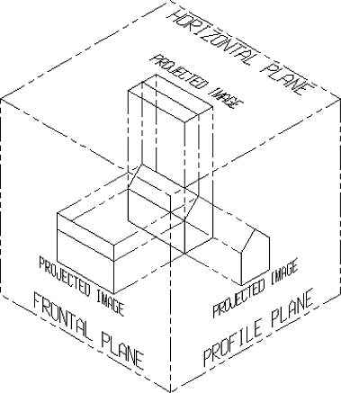

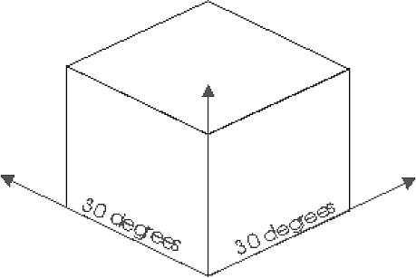


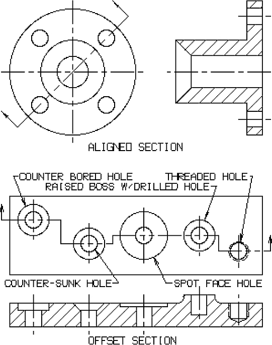


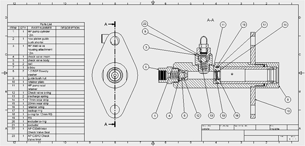
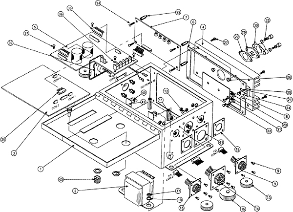


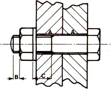
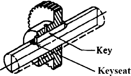
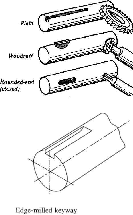


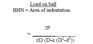
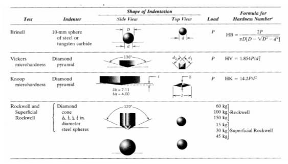

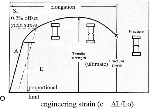
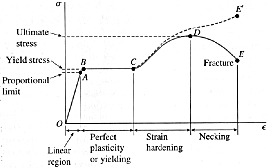

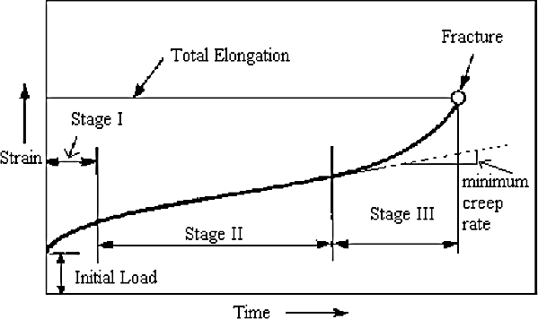


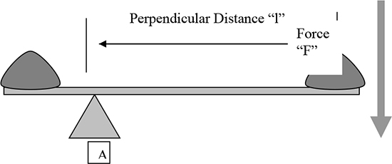


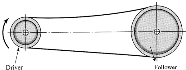


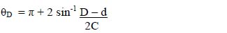


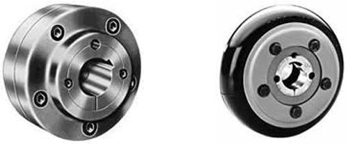


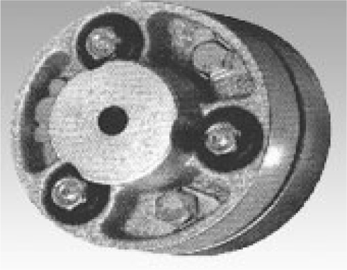

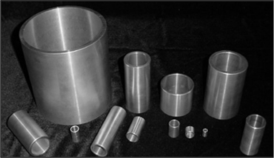
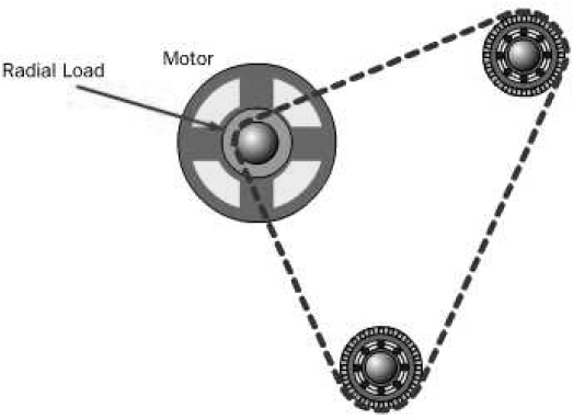


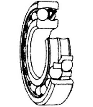
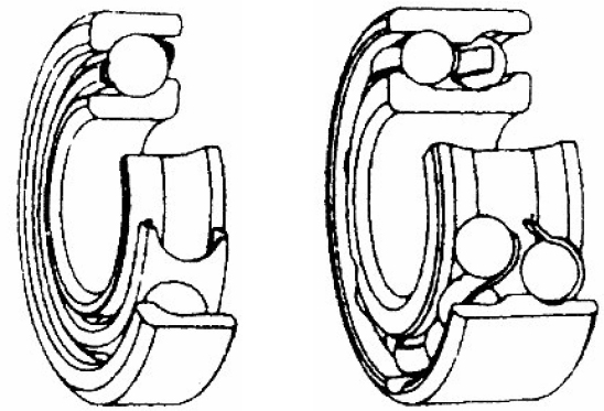
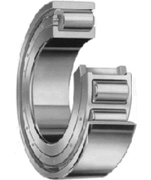
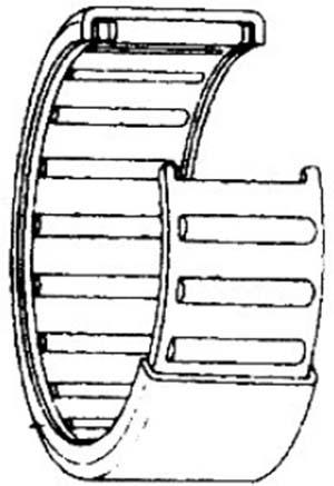


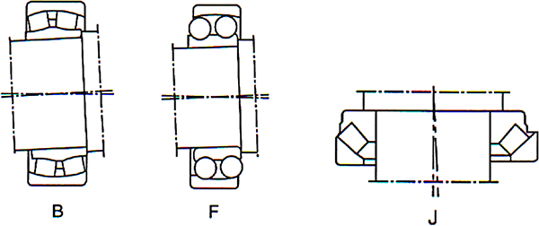


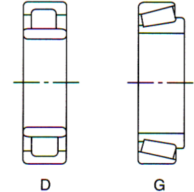
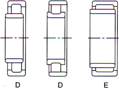


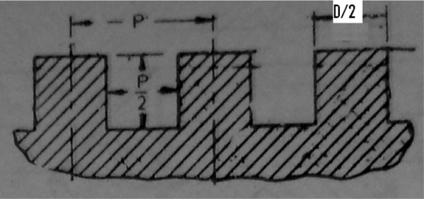
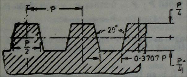
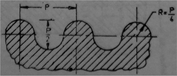
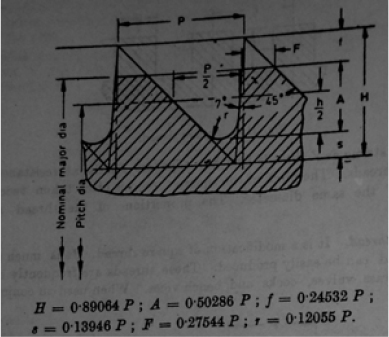

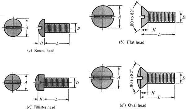
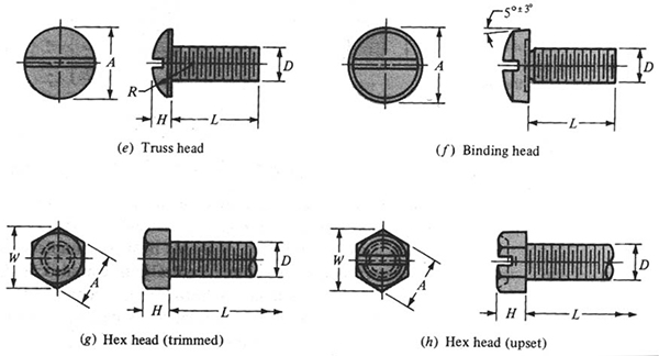


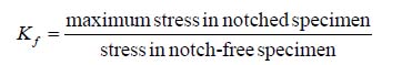
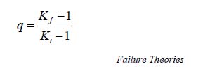


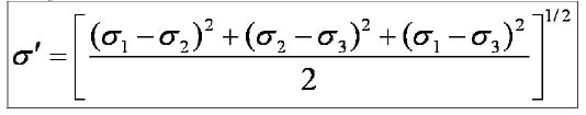
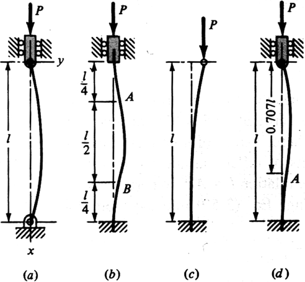
 This equation is called the Euler column formula or Euler’s Formula for columns. It applies only to rounded-end columns.

 and
and  . The variable stress in general may be considered as a combination of steady (or mean or average ) stress and a completely reversed stress component

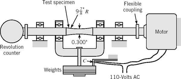
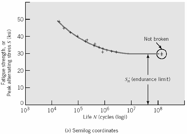


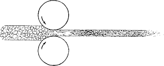


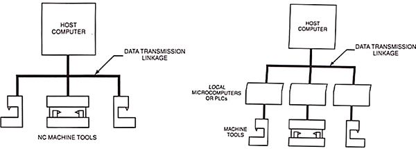


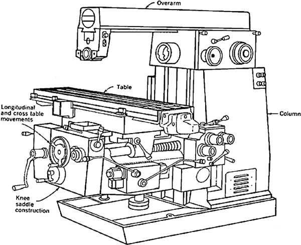


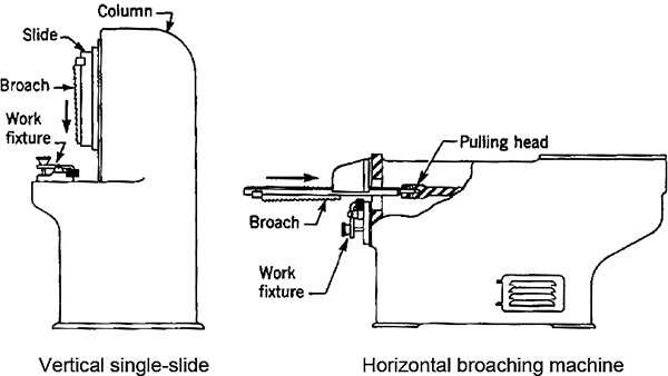


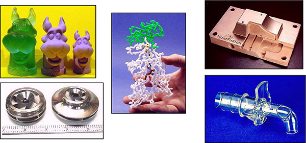
 ./
./
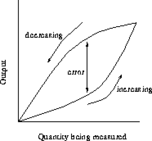


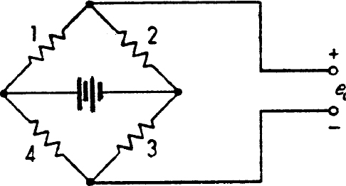
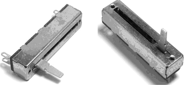


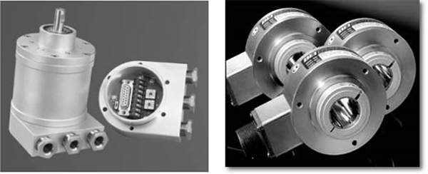

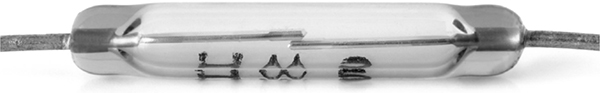


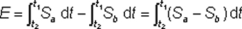


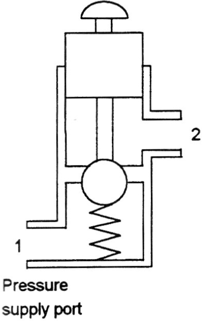

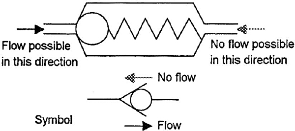


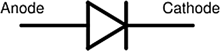

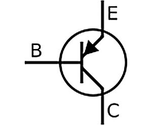


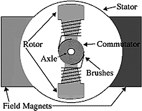
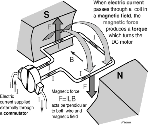

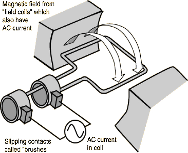
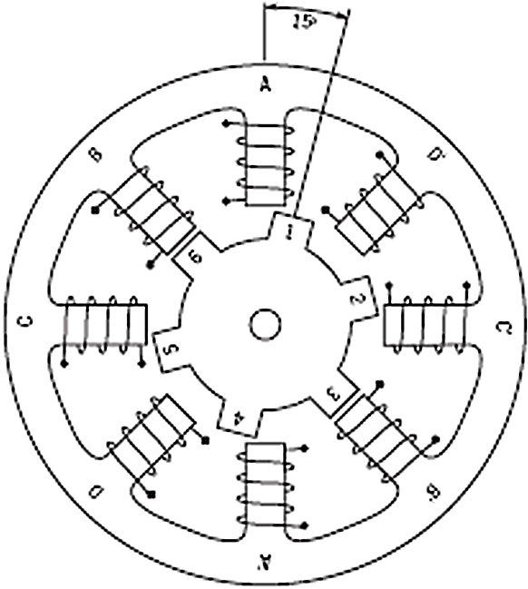

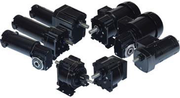

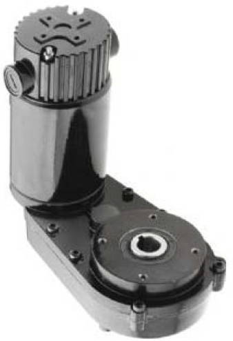


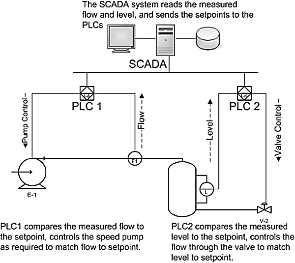

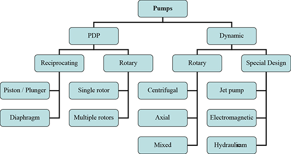


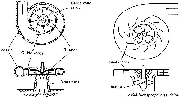


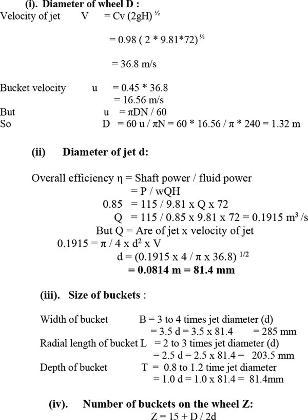


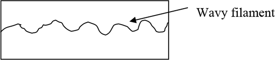


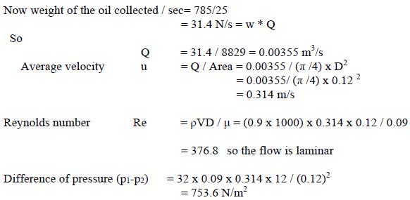


 Energy exhaust

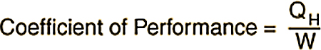
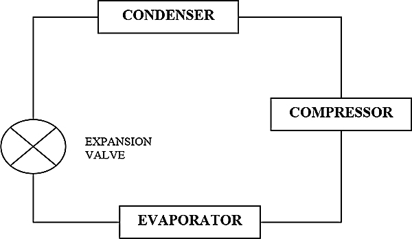

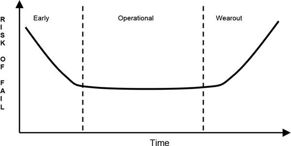


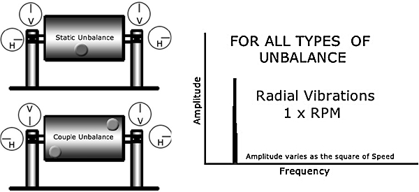


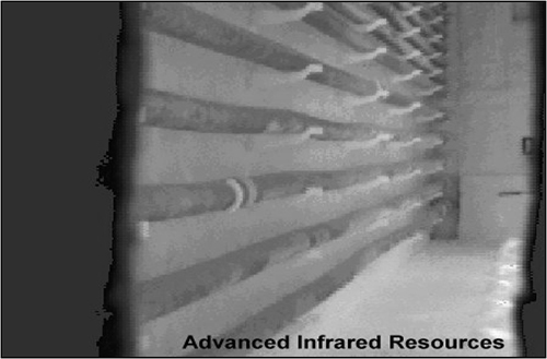
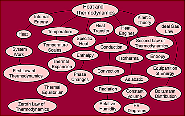


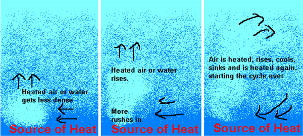

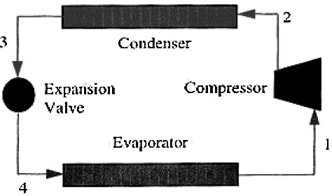
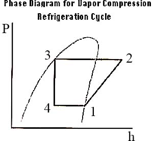


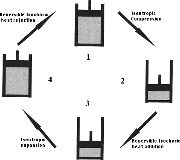
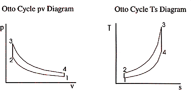

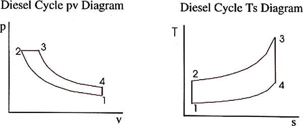


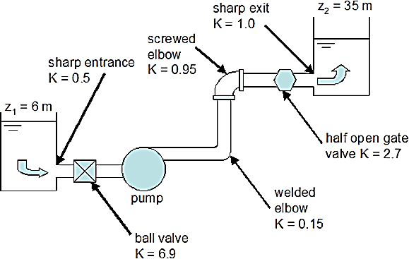

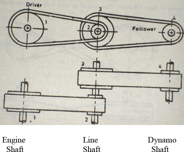


")


")


 & SCADA Systems")


")
")


")
